Quasi-one- and quasi-two-dimensional perfect Bose gas: the second critical density and generalised condensation

Abstract

In this letter we discuss a relevance of the 3D Perfect Bose gas (PBG) condensation in extremely elongated vessels for the study of anisotropic condensate coherence and the ”quasi-condensate”. To this end we analyze the case of exponentially anisotropic (van den Berg) boxes, when there are two critical densities $\rho_{c}<\rho_{m}$ for a generalised Bose-Einstein Condensation (BEC). Here $\rho_{c}$ is the standard critical density for the PBG. We consider three examples of anisotropic geometry: slabs, squared beams and ”cigars” to demonstrate that the ”quasi-condensate” which exists in domain $\rho_{c}<\rho<\rho_{m}$ is in fact the van den Berg-Lewis-Pulé generalised condensation (vdBLP-GC) of the type III with no macroscopic occupation of any mode.

We show that for the slab geometry the second critical density $\rho_{m}$ is a threshold between quasi-two-dimensional (quasi-2D) condensate and the three dimensional (3D) regime when there is a coexistence of the ”quasi-condensate” with the standard one-mode BEC. On the other hand, in the case of squared beams and ”cigars” geometries critical density $\rho_{m}$ separates quasi-1D and 3D regimes. We calculate the value of difference between $\rho_{c}$, $\rho_{m}$ (and between corresponding critical temperatures $T_{m}$, $T_{c}$) to show that observed space anisotropy of the condensate coherence can be described by a critical exponent $\gamma(T)$ related to the anisotropic ODLRO. We compare our calculations with physical results for extremely elongated traps that manifest ”quasi-condensate”.

1.One can rigorously show that there is no a conventional Bose-Einstein condensation (BEC) in the one- ($1D$) and two-dimensional ($2D$) boson systems or in the three-dimensional squared beams (cylinders) and slabs (films). For interacting Bose-gas it results from the Bogoliubov-Hohenberg theorem Bog62 , Hoh , based on a non-trivial Bogoliubov inequality, see e.g. BoMa . For the perfect Bose-gas this result is much easier, since it follows from the explicit analysis of the occupation number density in one-particle eigenstates. A common point is the Bogoliubov $1/q^{2}$-theorem Bog62 , Bog-Selv2 , Bog-v6-II , which implies destruction of the macroscopic occupation of the ground-state by thermal fluctuations.

Renewed interest to eventual possibility of the ”condensate” in the quasi-one-, or -two-dimensional (quasi-$1D$ or -$2D$) boson gases (i.e., in cigar-shaped systems or slabs) is motivated by recent experimental data indicating the existence of so-called ”quasi-condensate” in anisotropic traps Gerbier -Petrov1 and BKT crossover Dalibard .

The aim of this letter is twofold. First we show that a natural modeling of slabs by highly anisotropic $3D$-cuboid implies in the thermodynamic limit the van den Berg-Lewis-Pulé generalised condensation (vdBLP-GC) vdBLP of the Perfect Bose-Gas (PBG) for densities larger than the first, i.e. the standard critical $\rho_{c}(\beta)$ for the inverse temperature $\beta=1/(k_{B}T)$. Notice, that a special case of this (induced by the geometry) condensation was pointed out for the first time by Casimir Cas , although the theoretical concept and the name are due to Girardeau Gir . So, for the PBG the ”quasi-condensate” is in fact the vdBLP-GC. Here we generalise these results to the highly anisotropic $3D$-cuboid with anisotropy in one-dimension, which is a model for infinite squared beams or cylinders, and ”cigar” type traps.
Second, we show that for the slab geometry with exponential growing (for $\alpha>0$ and $L\rightarrow\infty$) of two edges, $L_{1}=L_{2}=Le^{\alpha L}$, $L_{3}=L$, of the anisotropic boxes: $\Lambda=L_{1}\times L_{2}\times L_{3}\in\mathbb{R}^{3}$, there is a second critical density $\rho_{m}(\beta):=\rho_{c}(\beta)+2\alpha/\lambda_{\beta}^{2}\geq\rho_{c}(\beta)$ such that the vdBLP-GC changes its properties when $\rho>\rho_{m}(\beta)$. This surprising behaviour of the BEC for the PBG was discovered by van den Berg vdB , developed in vdBLL , and then in GP ,Pa for the spin-wave condensation.

Notice that the exponential anisotropy is not a very common concept for the experimental implementations. Therefore, it appeals for a re-examination of the standard vdBLP-GC concept in Casimir boxes Beau and the corresponding version of the Bogoliubov-Hohenberg theorem MuHoLa .

Our original observation concerns the coexistence of two types of the vdBLP-GC for $\rho>\rho_{m}(\beta)$ (or for corresponding temperatures $T<T_{m}(\rho)$ for a fixed density) and the analysis of the coherence length (ODLRO) in this anisotropic geometry. We extend also our observation to obtain another new result proving the existence of the second critical density in the squared beam and in the ”cigar” type traps for exponentially weak harmonic potential confinement in one direction. We use these results to calculate the temperature dependence of the vdBLP-GC particle density for the case of two critical densities, $\rho_{m}(\beta){>}\rho_{c}(\beta)$ and to apply the recent scaling approach Beau to the ODLRO asymptotic in this case.

2. It is known that all kinds of BEC in the PBG are defined by the limiting spectrum of the one-particle Hamiltonian $T_{\Lambda}^{(N=1)}=-{\hbar^{2}}\Delta/({2m})$, when cuboid $\Lambda\uparrow{\mathbb{R}}^{3}$. In this paper we make this operator self-adjoint by fixing the Dirichlet boundary conditions on $\partial\Lambda$, although our results are valid for all non-attractive boundary conditions. Then the spectrum is the set

$$\{\varepsilon_{s}=\frac{\hbar^{2}}{2m}\sum_{j=1}^{3}(\pi s_{j}/L_{j})^{2}\}_{s_{j}\in\mathbb{N}}$$ (1)

and $\{\phi_{s,\Lambda}(x)=\prod_{j=1}^{3}\sqrt{2/L_{j}}\sin(\pi s_{j}x_{j}/L_{j})\}_{s_{j}\in\mathbb{N}}$ are the eigenfunctions. Here $\mathbb{N}$ is the set of the natural numbers and $s=(s_{1},s_{2},s_{3})\in\mathbb{N}^{3}$ is the multi-index.

In the grand-canonical ensemble $(T,V,\mu)$, here $V=L_{1}L_{2}L_{3}$ is the volume of $\Lambda$, the mean occupation number of the state $\phi_{s,\Lambda}$ is $N_{s}(\beta,\mu)=(e^{\beta(\varepsilon_{s}-\mu)}-1)^{-1}$, where $\mu<\inf_{s}\varepsilon_{s,\Lambda}$. Then for the fixed total particle density $\rho$ the corresponding value of the chemical potential $\mu_{\Lambda}(\beta,\rho)$ is a unique solution of the equation $\rho=\sum_{s\in{\mathbb{N}}^{3}}N_{s}(\beta,\mu)/V=:N_{\Lambda}(\beta,\mu)/V$. Independent of the way $\Lambda\uparrow{\mathbb{R}}^{3}$, one gets the limit $\rho(\beta,\mu)=\lim_{V\rightarrow\infty}N_{\Lambda}(\beta,\mu)/V$, which is the total particle density for $\mu\leq\lim_{V\rightarrow\infty}\inf_{s}\varepsilon_{s}=0$. Since $\rho_{c}(\beta):=\sup_{\mu\leq 0}\rho(\beta,\mu)=\rho(\beta,\mu=0)<\infty$, it is the (first) critical density for the $3D$ PBG: $\rho_{c}(\beta)={\zeta(3/2)}/{\lambda_{\beta}^{3}}$. Here $\zeta(s)$ is the Riemann $\zeta$-function and $\lambda_{\beta}:=\hbar\sqrt{{2\pi\beta}/{m}}$ is the de Broglie thermal length.

3. For $\Lambda=Le^{\alpha L}\times Le^{\alpha L}\times L$ one gets (vdB ; vdBLL ) that for any $\mu\leq 0$ the limit of Darboux-Riemann sums

$$\lim_{L\rightarrow\infty}\sum_{s\neq(s_{1},s_{2},1)}\frac{N_{s}(\beta,\mu)}{V_{L}}=\frac{1}{(2\pi)^{3}}\int_{\mathbb{R}^{3}}\frac{d^{3}k}{e^{\beta(\hbar^{2}k^{2}/2m-\mu)}-1}\ .$$ (2)

We denote by $\mu_{L}(\beta,\rho):=\varepsilon_{(1,1,1)}-\Delta_{L}(\beta,\rho)$, where $\Delta_{L}(\beta,\rho)\geq 0$ is a unique the solution of the equation:

$$\rho=\sum_{s=(s_{1},s_{2},1)}\frac{N_{s}(\beta,\mu)}{V_{L}}+\sum_{s\neq(s_{1},s_{2},1)}\frac{N_{s}(\beta,\mu)}{V_{L}}.$$ (3)

Since by (2): $\lim_{L\rightarrow\infty}\sum_{s\neq(s_{1},s_{2},1)}{N_{s}(\beta,\mu=0)}/{V_{L}}=\rho_{c}(\beta)$, for $\rho>\rho_{c}(\beta)$ the limit $L\rightarrow\infty$ of the first sum in (3) is equal to

$$\lim_{L\rightarrow\infty}\sum_{s=(s_{1},s_{2},1)}\frac{N_{s}(\beta,\mu)}{V_{L}}=$$

$$\lim_{L\rightarrow\infty}\frac{1}{L}\frac{1}{(2\pi)^{2}}\int_{\mathbb{R}^{2}}\frac{d^{2}k}{e^{\beta(\hbar^{2}k^{2}/2m+\Delta_{L}(\beta,\rho))}-1}=$$

$$\lim_{L\rightarrow\infty}-\frac{1}{\lambda_{\beta}^{2}L}\ln[\beta\Delta_{L}(\beta,\rho)]=\rho-\rho_{c}(\beta).$$

This implies the asymptotics:

$$\Delta_{L}(\beta,\rho)=\frac{1}{\beta}\ e^{-\lambda_{\beta}^{2}(\rho-\rho_{c}(\beta))L}+\ldots\ .$$ (5)

Notice that representation of the limit (Quasi-one- and quasi-two-dimensional perfect Bose gas: the second critical density and generalised condensation) by the integral (see (1)) is valid only when $\lambda_{\beta}^{2}(\rho-\rho_{c}(\beta))<2\alpha$. For $\rho$ larger than the second critical density: $\rho_{m}(\beta):=\rho_{c}(\beta)+2\alpha/\lambda_{\beta}^{2}$ the correction $\Delta_{L}(\beta,\rho)$ must converge to zero faster than $e^{-2\alpha L}$. Now to keep the difference $\rho-\rho_{m}(\beta)>0$ we have to return back to the original sum representation (3) and (as for the standard BEC) to take into account the impact of the ground state occupation density together with a saturated non-ground state (i.e. generalised) condensation $\rho_{m}(\beta)-\rho_{c}(\beta)$ as in (Quasi-one- and quasi-two-dimensional perfect Bose gas: the second critical density and generalised condensation). For this case the asymptotics of $\Delta_{L}(\beta,\rho>\rho_{m}(\beta))$ is completely different than (5) and it is equal to $\Delta_{L}(\beta,\rho)=[\beta(\rho-\rho_{m}(\beta))V_{L}]^{-1}$. Since $V_{L}=L^{3}e^{2\alpha L}$, we obtain:

$$\lim_{L\rightarrow\infty}\sum_{s=(s_{1}>1,s_{2}>1,1)}\frac{N_{s}(\beta,\mu)}{V_{L}}=$$ (6)

$$\lim_{L\rightarrow\infty}-\frac{1}{\lambda_{\beta}^{2}L}\ln[\beta\Delta_{L}(\beta,\rho)]=2\alpha/\lambda_{\beta}^{2}=$$

$$\rho_{m}(\beta)-\rho_{c}(\beta),$$

and the ground-state term gives the macroscopic occupation:

$$\rho-\rho_{m}(\beta)=\lim_{L\rightarrow\infty}\frac{1}{V_{L}}\frac{1}{e^{\beta(\varepsilon_{(1,1,1)}-\mu_{L}(\beta,\rho))}-1}\ .$$ (7)

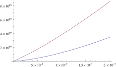
Figure 1: For the slab geometry, the blue curve $\rho_{c}(1/(k_{B}T))$ is the first critical line for the BEC transition as a function of $T$, the red curve $\rho_{m}(1/(k_{B}T))=\rho_{c}(1/(k_{B}T))+2\alpha/\lambda^{2}_{\beta}$ is the second critical line. Notice that above the red curve there is a coexistence between ”quasi-condensate” (vdBLP-GC of type III) and the conventional condensate in the ground state (vdBLP-GC of type I), between two curve there is only ”quasi-condensates” phase and below the blue curve there is no condensate.

Notice that for $\rho_{c}(\beta)<\rho<\rho_{m}(\beta)$ we obtain the vdBLP-GC (of the type III), i.e. none of the single-particle states are macroscopically occupied, since by virtue of (1) and (5) for any $s$ one has:

$$\rho_{s}(\beta,\rho):=\lim_{L\rightarrow\infty}\frac{1}{V_{L}}\frac{1}{e^{\beta(\varepsilon_{s}-\mu_{L}(\beta,\rho))}-1}=0\ .$$ (8)

On the other hand, the asymptotics $\Delta_{L}(\beta,\rho>\rho_{m}(\beta))=[\beta(\rho-\rho_{m}(\beta))V_{L}]^{-1}$ implies

$$\rho_{s\neq(1,1,1)}(\beta,\rho):=\lim_{L\rightarrow\infty}\frac{1}{V_{L}}\frac{1}{e^{\beta(\varepsilon_{s}-\mu_{L}(\beta,\rho))}-1}=0\ ,$$ (9)

i.e. for $\rho>\rho_{m}(\beta)$ there is a coexistence of the saturated type III vdBLP-GC, with the constant density (6), and the standard BEC (i.e. the type I vdBLP-GC) in the single state (7).

4. It is curious to note that neither Casimir shaped boxes vdBLP , nor the van den Berg boxes $\Lambda=Le^{\alpha L}\times L\times L$, with one-dimensional anisotropy do not produce the second critical density $\rho_{m}(\beta)\neq\rho_{c}(\beta)$. To model infinite squared beams with BEC transitions at two critical densities we propose the one-particle Hamiltonian: $T_{\Lambda}^{(N=1)}=-{\hbar^{2}}\Delta/({2m})+m\omega^{2}_{1}x_{1}^{2}/2$, with harmonic trap in direction $x_{1}$ and, e.g., Dirichlet boundary conditions in directions $x_{2},x_{3}$. Then the spectrum is the set

$$\{\epsilon_{s}:=\hbar\omega_{1}(s_{1}+{1}/{2})+\frac{\hbar^{2}}{2m}\sum_{j=2}^{3}(\pi s_{j}/L_{j})^{2}\}_{s\in\mathbb{N}}.$$ (10)

Here multi-index $s=(s_{1},s_{2},s_{3})\in(\mathbb{N}\cup\{0\})\times\mathbb{N}^{2}$, and the ground-state energy is $\epsilon_{(0,1,1)}$. Then for $\mu_{L}(\beta,{\varrho}):=\epsilon_{(0,1,1)}-\Delta_{L}(\beta,{\varrho})$, the value of $\Delta_{L}(\beta,{\varrho})\geq 0$, is a solution of the equation:

$${\varrho}:=\sum_{s=(s_{1},1,1)}\omega_{1}\frac{N_{s}(\beta,\mu)}{L_{2}L_{3}}+\sum_{s\neq(s_{1},1,1)}\omega_{1}\frac{N_{s}(\beta,\mu)}{L_{2}L_{3}},$$ (11)

where $N_{s}(\beta,\mu)=(e^{\beta(\epsilon_{s}-\mu)}-1)^{-1}$.

Let $\omega_{1}:=\hbar/(mL_{1}^{2})$ and $L_{2}=L_{3}=L$. Here $L_{1}$ is the harmonic-trap characteristic size in direction $x_{1}$. Then for any $s_{1}\geq 0$ and $\mu\leq 0$

$$\varrho(\beta,\mu):=\lim_{L_{1},L\rightarrow\infty}\sum_{s\neq(s_{1},1,1)}\omega_{1}\frac{N_{s}(\beta,\mu)}{L_{2}L_{3}}=$$

$$\frac{1}{(2\pi)^{2}}\int_{0}^{\infty}dp\int_{\mathbb{R}^{2}}\frac{d^{2}k}{e^{\beta(\hbar p+\hbar^{2}k^{2}/2m-\mu)}-1}\ .$$ (12)

Therefore, the first critical density is finite: $\varrho_{c}(\beta):=\sup_{\mu\leq 0}\varrho(\beta,\mu)=\varrho(\beta,\mu=0)<\infty$. If $\varrho>\varrho_{c}(\beta)$, then the limit $L\rightarrow\infty$ of the first sum in (11) is

$$\lim_{L_{1},L\rightarrow\infty}\sum_{s=(s_{1},1,1)}\omega_{1}\frac{N_{s}(\beta,\mu_{L})}{L_{2}L_{3}}=$$

$$\lim_{L\rightarrow\infty}\frac{1}{L^{2}}\int_{0}^{\infty}\frac{dp}{e^{\beta(\hbar p+\Delta_{L}(\beta,{\varrho}))}-1}=$$

$$\lim_{L\rightarrow\infty}-\frac{1}{\hbar\beta L^{2}}\ln[\beta\Delta_{L}(\beta,{\varrho})]={\varrho}-\varrho_{c}(\beta).$$

This means that the asymptotics of $\Delta_{L}(\beta,\rho)$ is:

$$\Delta_{L}(\beta,{\varrho})=\frac{1}{\beta}\ e^{-\hbar\beta({\varrho}-\varrho_{c}(\beta))L^{2}}+\ldots\ .$$ (14)

Let $L_{1}:=Le^{\gamma L^{2}}$, for $\gamma>0$. Then, similar to our arguments in 2., the representation of the limit (Quasi-one- and quasi-two-dimensional perfect Bose gas: the second critical density and generalised condensation) by the integral is valid for $\hbar\beta(\varrho-\varrho_{c}(\beta))<2\gamma$. For ${\varrho}$ larger than the second critical density: $\varrho_{m}(\beta):=\varrho_{c}(\beta)+2\gamma/(\hbar\beta)$ the chemical potential correction (14) must converge to zero faster than $e^{-2\gamma L^{2}}$. By the same line of reasoning as in 2., to keep the difference ${\varrho}-\varrho_{m}(\beta)>0$ we have to use the original sum representation (11) and to take into account the input due to the ground state occupation density together with a saturated non-ground state condensation $\varrho_{m}(\beta)-\varrho_{c}(\beta)$ (Quasi-one- and quasi-two-dimensional perfect Bose gas: the second critical density and generalised condensation). The asymptotics of $\Delta_{L}(\beta,{\varrho}>\varrho_{m}(\beta))$ is than equal to $\Delta_{L}(\beta,{\varrho})=[\beta m({\varrho}-\varrho_{m}(\beta))L^{4}e^{2\gamma L^{2}}/\hbar]^{-1}$. Hence,

$$\lim_{L\rightarrow\infty}\sum_{s=(s_{1}>0,1,1)}\frac{\hbar}{m}\ \frac{N_{s}(\beta,\mu_{L})}{L^{4}e^{2\gamma L^{2}}}=$$ (15)

$$\lim_{L\rightarrow\infty}-\frac{1}{\hbar\beta L^{2}}\ln[\beta\Delta_{L}(\beta,{\varrho})]=\frac{2\gamma}{\hbar\beta}=\varrho_{m}(\beta)-\varrho_{c}(\beta),$$

and the ground-state term gives the macroscopic occupation:

$${\varrho}-\varrho_{m}(\beta)=\lim_{L\rightarrow\infty}\frac{\hbar}{mL^{4}e^{2\gamma L^{2}}}\frac{1}{e^{\beta(\epsilon_{(0,1,1),L}-\mu_{L}(\beta,{\varrho}))}-1}\ .$$ (16)

With this choice of boundary conditions and the one-dimensional anisotropic trap our model of the infinite squared beams manifests the BEC with two critical densities. Again for $\varrho_{c}(\beta)<{\varrho}<\varrho_{m}(\beta)$ we obtain the type III vdBLP-GC, i.e., none of the single-particle states are macroscopically occupied:

$$\varrho_{s}(\beta,{\varrho}):=\lim_{L\rightarrow\infty}\frac{\hbar}{mL^{4}e^{2\gamma L^{2}}}\frac{1}{e^{\beta(\epsilon_{s}-\mu_{L}(\beta,{\varrho}))}-1}=0\ .$$ (17)

When $\varrho_{m}(\beta)<{\varrho}$ there is a coexistence of the type III vdBLP-GC, with the constant density (Quasi-one- and quasi-two-dimensional perfect Bose gas: the second critical density and generalised condensation), and the standard type I vdBLP-GC in the single state (16), since

$$\varrho_{s\neq(0,1,1)}(\beta,{\varrho}):=\lim_{L\rightarrow\infty}\frac{\hbar}{mL^{4}e^{2\gamma L^{2}}}\frac{1}{e^{\beta(\epsilon_{s}-\mu_{L}(\beta,{\varrho}))}-1}=0\ .$$ (18)

Finally, it is instructive to study a ”cigar”-type geometry ensured by the anisotropic harmonic trap:

$$T_{\Lambda}^{(N=1)}=-{\hbar^{2}}\Delta/({2m})+\sum_{1\leq j\leq 3}m\omega^{2}_{j}x_{j}^{2}/2\ .$$ (19)

with $\omega_{1}=\hbar/(mL_{1}^{2}),\omega_{2}=\omega_{3}=\hbar/(mL^{2})$. Here $L_{1},L_{2}=L_{3}=L$ are the characteristic sizes of the trap in three directions and $\eta_{s}=\sum_{1\leq j\leq 3}\hbar\omega_{j}(s_{j}+{1}/{2})$ is the corresponding one-particle spectrum. Then the same reasoning as in (12),(Quasi-one- and quasi-two-dimensional perfect Bose gas: the second critical density and generalised condensation), yields for $\mu_{L}(\beta,{n}):=\eta_{(0,0,0)}-\Delta_{L}(\beta,{n})$ and auxiliary dimensionality factor $\kappa>0$:

$$\lim_{L_{1},L\rightarrow\infty}\sum_{s=(s_{1},0,0)}\kappa^{3}\omega_{1}\omega_{2}\omega_{3}{N_{s}(\beta,\mu_{L})}=$$

$$\lim_{L\rightarrow\infty}-\frac{\kappa^{3}\hbar}{\beta(mL^{2})^{2}}\ln[\beta\Delta_{L}(\beta,{n})]={n}-n_{c}(\beta).$$

Here the finite critical density $n_{c}(\beta):=n(\beta,\mu=0)$ is defined similarly to (12), where the particle density is

$$n(\beta,\mu):=\lim_{L_{1},L\rightarrow\infty}\sum_{s\neq(s_{1},0,0)}\kappa^{3}\omega_{1}\omega_{2}\omega_{2}{N_{s}(\beta,\mu)}=$$

$$\int_{{\mathbb{R}^{3}}_{+}}\frac{\kappa^{3}d{\omega}_{1}d{\omega}_{2}d{\omega}_{3}}{e^{\beta[\hbar({\omega}_{1}+{\omega}_{2}+{\omega}_{3})-\mu]}-1}\ .$$ (21)

Equation (Quasi-one- and quasi-two-dimensional perfect Bose gas: the second critical density and generalised condensation) implies for $\Delta_{L}(\beta,{n})$ the same asymptotics as in (Quasi-one- and quasi-two-dimensional perfect Bose gas: the second critical density and generalised condensation):

$$\Delta_{L}(\beta,{n})=\frac{1}{\beta}\ e^{-\beta({n}-n_{c}(\beta))m^{2}L^{4}/(\hbar\kappa^{3})}+\ldots\ .$$ (22)

If we choose $L_{1}:=Le^{\widehat{\gamma}L^{4}}$, for $\widehat{\gamma}>0$, then the second critical density $n_{m}(\beta):=n_{c}(\beta)+(\widehat{\gamma}\hbar\kappa^{3})/(\beta m^{2})$. For $n_{c}(\beta)<{n}<n_{m}(\beta)$ we obtain the type III vdBLP-GC, i.e., none of the single-particle states are macroscopically occupied:

$$n_{s}(\beta,n):=\lim_{L\rightarrow\infty}\frac{\kappa^{3}\,\omega_{1}\omega_{2}\omega_{3}}{e^{\beta(\eta_{s}-\mu_{L}(\beta,{n}))}-1}=0\ .$$ (23)

Although for $n_{m}(\beta)<n$ there is a coexistence of the type III vdBLP-GC, with the constant density $n_{m}(\beta)-n_{c}(\beta)$, and the standard type I vdBLP-GC in the ground-state:

$${n}-n_{m}(\beta)=\lim_{L\rightarrow\infty}\frac{\kappa^{3}\,\omega_{1}\omega_{2}\omega_{3}}{e^{\beta(\eta_{(0,0,0)}-\mu_{L}(\beta,{n}))}-1}\ .$$ (24)

5. In experiments with BEC, it is important to know the critical temperatures associated with corresponding critical densities. The first critical temperatures: $T_{c}(\rho)$, $\widetilde{T}_{c}(\rho)$ or $\widehat{T}_{c}(\rho)$ are well-known. For a given density $\rho$ they verify the identities:

$$\rho=\rho_{c}(\beta_{c}(\rho))\ ,\ \varrho=\varrho_{c}(\widetilde{\beta}_{c}(\varrho))\ ,\ n=n_{c}(\widehat{\beta}_{c}(n))\ ,$$ (25)

respectively for our models of slabs, squared beams or ”cigars”. Since definition of the critical densities yield the representations: $\rho_{c}(\beta)=:T^{3/2}\,I_{sl}$, $\varrho_{c}(\beta)=:T^{2}\,I_{bl}$, $n_{c}(\beta)=:T^{3}\,I_{cg}$, the expressions for the second critical densities one gets the following relations between the first and the second critical temperatures:

$$T_{m}^{3/2}(\rho)+{{\tau}^{1/2}}\ T_{m}(\rho) = T_{c}^{3/2}(\rho)\ \ {\rm{(slab)}}\ ,$$

$$\widetilde{T}_{m}^{2}({\varrho})+{\widetilde{\tau}}\ \widetilde{T}_{m}({\varrho}) = \widetilde{T}_{c}^{2}({\varrho})\ \ \ \ {\rm{(beam)}}\ ,$$

$$\widehat{T}_{m}^{3}({n})+{\widehat{\tau}}^{2}\ \widehat{T}_{m}({n}) = \widehat{T}_{c}^{3}({n})\ \ \ \ {\rm{(cigar)}}\ .$$

Here $\tau=[\alpha mk_{B}/(\pi\hbar^{2}I_{sl})]^{2}$, $\widetilde{\tau}=2\gamma k_{B}/(\hbar I_{bl})$ and $\widehat{\tau}=[(\widehat{\gamma}\hbar\kappa^{3}k_{B})/(m^{2}I_{cg})]^{1/2}$ are ”effective” temperatures related to the corresponding geometrical shapes.

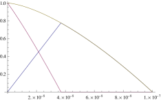
Figure 2: The first (blue fit) , The second (pink fit) and the total (green fit) condensate fractions as a function of the temperature for ${}^{87}Rb$ atoms in the slab geometry with $T_{c_{1}}=10^{-7}K$ and $\tau=4.43\times 10^{-7}$.

Notice that the second critical temperature modifies the usual law for the condensate fractions temperature dependence, since now the total condensate density is $\rho-\rho_{c}(\beta):=\rho_{0}(\beta)=\rho_{0c}(\beta)+\rho_{0m}(\beta)$. Here $\rho_{0m}(\beta):=(\rho-\rho_{m}(\beta))\ \theta(\rho-\rho_{m}(\beta))$.

For example, in the case of the slab geometry the type III vdBLP-GC (i.e. the ”quasi-condensate”) $\rho_{0c}(\beta)$ behaves for a given $\rho$ like (see Fig.2.)

$$\frac{\rho_{0c}(\beta)}{\rho}=\left\{\begin{array}[]{ll}1-(T/T_{c})^{3/2}\ ,&\textrm{~{}~{}~{}~{}~{}$T_{m}\leq T\leq T_{c}$ },\\ {\sqrt{\tau}\ T}/{T_{c}^{3/2}}\ \ \ \ ,&\textrm{~{}~{}~{}~{}~{}$T\leq T_{m}$ }.\end{array}\right.$$ (26)

Similarly, for the type I vdBLP-GC in the ground state $\rho_{0m}(\beta)$ (i.e. the conventional BEC) we obtain:

$$\frac{\rho_{0m}(\beta)}{\rho}=\left\{\begin{array}[]{ll}0\ ,&\textrm{$T_{m}\leq T\leq T_{c}$},\\ 1-(T/T_{c})^{3/2}(1+\sqrt{{\tau}/{T}}),&\textrm{$T\leq T_{m}$},\end{array}\right.$$ (27)

see Fig.2. The total condensate density $\rho_{0}(\beta):=\rho_{0c}(\beta)+\rho_{0m}(\beta)$ is the result of coexistence of both of them: it gives the standard PBG expression $\rho_{0}(\beta)/\rho=1-(T/T_{c})^{3/2}$.

For the ”cigars” geometry case the temperature dependence of the ”quasi-condensate” $r_{0c}(\beta)$ is

$$\frac{n_{0c}(\beta)}{{n}}=\left\{\begin{array}[]{ll}1-(T/\widehat{T}_{c})^{3}\ ,&\textrm{~{}~{}~{}~{}~{}$\widehat{T}_{m}\leq T\leq\widehat{T}_{c}$ },\\ {{\widehat{\tau}}^{2}\ T}/{\widehat{T}_{c}^{3}}\ \ \ \ \ \ ,&\textrm{~{}~{}~{}~{}~{}$T\leq\widehat{T}_{m}$ }.\end{array}\right.$$ (28)

The corresponding ground state conventional BEC behaves as

$$\frac{n_{0m}(\beta)}{{n}}=\left\{\begin{array}[]{ll}0\ ,&\textrm{${\widehat{T}}_{m}\leq T\leq{\widehat{T}}_{c}$},\\ 1-(T/\widehat{T}_{c})^{3}(1+{\widehat{\tau}}^{2}/{T^{2}}),&\textrm{$T\leq{\widehat{T}}_{m}$},\end{array}\right.$$ (29)

and again for the two coexisting condensates one gets ${n}-n_{c}(\beta):=n_{0}(\beta)=n_{0c}(\beta)+n_{0m}(\beta)=(1-(T/T_{c})^{3/2}){n}$.

Notice that for a given density the difference between two critical temperatures for the slab geometry can be calculated explicitly:

$$(T_{c}-T_{m})/T_{c}=g(\rho_{\alpha}/\rho)\ ,$$ (30)

where $\rho_{\alpha}:=8\alpha^{3}/\zeta(3/2)^{2}$ and $g(x)$ is an explicit algebraic function. For illustration consider a quasi-$2D$ PBG model of ${}^{87}Rb$ atoms in trap with characteristic sizes $L_{1}=L_{2}=100\mu m$, $L=1\mu m$ and with typical critical temperature $T_{c}=10^{-7}K$. The anisotropy parameter is $\alpha=(1/L)\ln(L_{1}/L)=4,6\cdot 10^{6}m^{-1}$. Then for ${\tau}=4,4\cdot 10^{-7}K$ we find $T_{m}=3,7\cdot 10^{-8}K$ and $(T_{c}-T_{m})/T_{c}=0,63$.

6. Another physical observable to characterise this second critical temperature is the condensate coherence length or the global spacial particle density distribution. The usual criterion is the ODLRO, which is going back to Penrose and Onsager PO . For a fixed particle density $\rho$ it is defined by the kernel:

$$K(x,y):=\lim_{L\rightarrow\infty}K_{\Lambda}(x,y)=\lim_{L\rightarrow\infty}\sum_{s}\frac{\overline{\phi}_{s,\Lambda}(x)\phi_{s,\Lambda}(y)}{e^{\beta(\varepsilon_{s}-\mu_{L}(\beta,\rho))}-1}\ .$$ (31)

The limiting diagonal function $\rho(x):=K(x,x)$ is local $x$-independent particle density.

To detect a trace of the geometry (or the second critical temperature) impact on the spatial density distribution we follow a recent scaling approach to the generalised BEC developed in Beau (see also vdBLP ,vdBLL ) and introduce a scaled global particle density:

$$\xi_{L}(u):=\sum_{s}\frac{|{\phi}_{s,\Lambda}(L_{1}u_{1},L_{2}u_{2},L_{3}u_{3})|^{2}}{e^{\beta(\varepsilon_{s}-\mu)}-1}\ ,$$ (32)

with the scaled distances $\{u_{j}=x_{j}/L_{j}\in[0,1]\}_{j=1,2,3}$.

For a given $\rho$ the scaled density (32) in the slab geometry is

$$\xi_{\rho,L}^{sl}(u):=\sum_{s}\frac{1}{e^{\beta(\varepsilon_{s}-\mu_{L}(\beta,\rho))}-1}\prod_{j=1}^{d=3}\frac{2}{L_{j}}[\sin(\pi s_{j}u_{j})]^{2}.$$ (33)

Since $2[\sin(\pi s_{j}u_{j})]^{2}=1-\cos\{(2\pi s_{j}/L_{j})u_{j}L_{j}\}$ and $\lim_{L\rightarrow\infty}\mu_{L}(\beta,\rho<\rho_{c}(\beta))<0$, by the Riemann-Lebesgue lemma we obtain that $\lim_{L\rightarrow\infty}\xi_{\rho,\Lambda}^{sl}(u)=\rho$ for any $u\in(0,1)^{3}$. If $\rho>\rho_{c}(\beta)$, one has to proceed as in (3)-(5). Then for any $u\in(0,1)^{3}$:

$$\lim_{L\rightarrow\infty}\sum_{s=(s_{1},s_{2},1)}\frac{1}{e^{\beta(\varepsilon_{s}-\mu_{L}(\beta,\rho))}-1}\prod_{j=1}^{d=3}\frac{2}{L_{j}}[\sin(\pi s_{j}u_{j})]^{2}$$

$$=\lim_{L\rightarrow\infty}\frac{2[\sin(\pi u_{3})]^{2}}{(2\pi)^{2}L}\int_{\mathbb{R}^{2}}\frac{\prod_{j=1}^{2}(1-\cos(2k_{j}u_{j}L_{j})d^{2}k}{e^{\beta(\hbar^{2}k^{2}/2m+\Delta_{L}(\beta,\rho))}-1}$$

$$=(\rho-\rho_{c}(\beta))\ 2[\sin(\pi u_{3})]^{2}\ ,$$ (34)

$$\lim_{L\rightarrow\infty}\sum_{s\neq(s_{1},s_{2},1)}\frac{1}{e^{\beta(\varepsilon_{s}-\mu_{L}(\beta,\rho))}-1}\prod_{j=1}^{d=3}\frac{2}{L_{j}}[\sin(\pi s_{j}u_{j})]^{2}$$

$$=\rho_{c}(\beta))\ .$$ (35)

Then the limit of (33) is equal to

$$\xi_{\rho}^{sl}(u)=(\rho-\rho_{c}(\beta))\ 2[\sin(\pi u_{3})]^{2}+\rho_{c}(\beta)\ .$$ (36)

It manifests a space anisotropy of the type III vdBLP-GC for $\rho_{c}(\beta)<\rho<\rho_{m}(\beta)$ in direction $u_{3}$.

For $\rho>\rho_{m}(\beta)$ one has to use representation (3) and asymptotics (6), (7). Then following the arguments developed above we obtain

$$\xi_{\rho}^{sl}(u)=(\rho-\rho_{m}(\beta))\prod_{j=1}^{3}\ 2[\sin(\pi u_{j})]^{2}+$$

$$(\rho_{m}(\beta)-\rho_{c}(\beta))\ 2[\sin(\pi u_{3})]^{2}+\rho_{c}(\beta)\ .$$ (37)

So, the anisotropy of the space particle distribution is still in direction $u_{3}$ due to the type III vdBLP-GC.

It is instructive to compare this anisotropy with a coherence length analysis within the scaling approach Beau to the BEC space distribution. To this end let us center the box $\Lambda$ at the origin of coordinates: $x_{j}=\tilde{x}_{j}+L_{j}/2$ and $y_{j}=\tilde{y}_{j}+L_{j}/2$. Then the ODLRO kernel (31) is:

$$K_{\Lambda}(\tilde{x},\tilde{y})=\sum_{l=1}^{\infty}e^{{l}\beta\mu_{L}(\beta,\rho)}\ R_{{l}}^{(2)}\ R_{{l}}^{(1)}\ ,$$ (38)

where after the shift of coordinates and using (1) we put

$$R_{{l}}^{(2)}(\tilde{x}^{(2)},\tilde{y}^{(2)})=$$ (40)

$$\sum_{s=(s_{1},s_{2})}e^{-{l}\beta\varepsilon_{s_{1},s_{2}}}\ \overline{\phi}_{s_{1},s_{2},\Lambda}(\tilde{x}_{1},\tilde{x}_{2})\ {\phi}_{s_{1},s_{2},\Lambda}(\tilde{y}_{1},\tilde{y}_{2})$$

$$R_{s}^{(1)}(\tilde{x}_{3},\tilde{y}_{3})=\sum_{s=(s_{3})}e^{-l\beta\varepsilon_{s_{3}}}\ \sqrt{\frac{2}{L_{3}}}\sin(\frac{\pi s_{3}}{L_{3}}(\tilde{x}_{3}+\frac{L_{3}}{2}))$$

$$\times\sqrt{\frac{2}{L_{3}}}\sin(\frac{\pi s_{3}}{L_{3}}(\tilde{y}_{3}+\frac{L_{3}}{2}))\ .$$

Similar to (3), for $\rho_{c}(\beta)<\rho<\rho_{m}(\beta)$ we must split the sum over $s=(s_{1},s_{2},s_{3})$ in (38) into two parts. Since by the generalized Weyl theorem one gets:

$$\lim_{L\rightarrow\infty}R_{{l}}^{(2)}(\tilde{x}^{(2)},\tilde{y}^{(2)})=\frac{1}{{l}\lambda_{\beta}^{2}}\ e^{-\pi\|\tilde{x}^{(2)}-\tilde{y}^{(2)}\|^{2}/{l}\lambda_{\beta}^{2}}\ ,$$

by (38) we obtain for the first part the representation:

$$\lim_{L\rightarrow\infty}\sum_{{l}=1}^{\infty}e^{{l}\beta\mu_{L}(\beta,\rho)}\sum_{s=(s_{1},s_{2},1)}e^{-{l}\beta\varepsilon_{s_{1},s_{2},1}}\times$$

$$\times\overline{\phi}_{s_{1},s_{2},1\Lambda}(\tilde{x})\ {\phi}_{s_{1},s_{2},1\Lambda}(\tilde{y})=$$

$$\lim_{L\rightarrow\infty}\sum_{{l}=1}^{\infty}e^{-{l}\beta\Delta_{L}(\beta,\rho)}\frac{1}{{l}\lambda_{\beta}^{2}}\ e^{-\pi\|\tilde{x}^{(2)}-\tilde{y}^{(2)}\|^{2}/{l}\lambda_{\beta}^{2}}\times$$

$$\times\frac{2}{L}\sin(\frac{\pi}{L}(\tilde{x}_{3}+\frac{L}{2}))\sin(\frac{\pi}{L}(\tilde{y}_{3}+\frac{L}{2}))\ .$$

For the second part we apply the Weyl theorem for the 3-dimensional Green function:

$$\lim_{L\rightarrow\infty}\sum_{{l}=1}^{\infty}e^{{l}\beta\mu_{L}(\beta,\rho)}\sum_{s\neq(s_{1},s_{2},1)}e^{-{l}\beta\varepsilon_{s}}\times$$

$$\times\overline{\phi}_{s,\Lambda}(\tilde{x})\ {\phi}_{s,\Lambda}(\tilde{y})=\sum_{{l}=1}^{\infty}\frac{1}{{l}\lambda_{\beta}^{3}}\ e^{-\pi\|\tilde{x}-\tilde{y}\|^{2}/{l}\lambda_{\beta}^{2}}\ .$$

If in (Quasi-one- and quasi-two-dimensional perfect Bose gas: the second critical density and generalised condensation) we change ${l}\rightarrow{l}\ \Delta_{L}(\beta,\rho)$, then it gets the form of the integral Darboux-Riemann sum, where $\|\tilde{x}^{(2)}-\tilde{y}^{(2)}\|^{2}$ is scaled as $\|\tilde{x}^{(2)}-\tilde{y}^{(2)}\|^{2}\ \Delta_{L}(\beta,\rho)$. Therefore, the coherence length $L_{ch}$ in direction perpendicular to $x_{3}$ is $L_{ch}(\beta,\rho)/L:=1/\sqrt{\Delta_{L}(\beta,\rho)}$. A similar argument is valid for $\rho>\rho_{m}(\beta)$ with obvious modifications due to BEC for $s=(1,1,1)$ (7) and to another asymptotics (6) for $\Delta_{L}(\beta,\rho)$. To compare the coherence length with the scale $L_{1,2}=Le^{\alpha L}$, let us define the critical exponent $\gamma(T,\rho)$ such that $\lim_{L\rightarrow\infty}(L_{ch}(\beta,\rho)/L)({L_{1}}/{L})^{-\gamma(T,\rho)}=1$. Then we get:

$$\gamma(T,\rho) = {\lambda_{\beta}^{2}}\ (\rho-\rho_{c}(\beta))/{2\alpha}\ ,\ \rho_{c}(\beta)<\rho<\rho_{m}(\beta)$$ (43)

$$= {\lambda_{\beta}^{2}}\ (\rho_{m}(\beta)-\rho_{c}(\beta))/{2\alpha}\ ,\ \rho_{m}(\beta)\leq\rho\ .$$

For a fixed density, taking into account (26) we find the temperature dependence of the exponent $\gamma(T):=\gamma(T,\rho)$, see Fig.3:

$$\gamma(T) = \sqrt{{T}/{\tau}}\ \{({T_{c}}/{T})^{3/2}-1\}\ ,\ T_{m}<T<T_{c}\ ,$$ (44)

$$= 1,\ T\leq T_{m}\ .$$

Notice that in the both cases the ODLRO kernel is anisotropic due to impact of the type III condensation (Quasi-one- and quasi-two-dimensional perfect Bose gas: the second critical density and generalised condensation) in the states $s=(s_{1},s_{2},1)$, whereas the other states give a symmetric part of correlations (Quasi-one- and quasi-two-dimensional perfect Bose gas: the second critical density and generalised condensation), which includes a constant term $\rho_{c}(\beta)$.

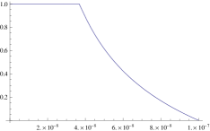
Figure 3: Exponent $\gamma(T)$ for evolution of the coherence length for the quasi-condensate with temperature corresponding to ${}^{87}Rb$ atoms in the slab geometry with $T_{c}=10^{-7}K$ and $\tau=4.43\times 10^{-7}K$

Numerically, for $L_{1}=L_{2}=100\mu m,\ L_{3}=1\mu m$ and $T_{m}<T=0.75T_{c}$ the coherence length of the condensate is equal to $2.8\mu m\ll 100\mu m$. This decreasing of the coherence length is experimentally observed in Gerbier .

7. In conclusion we add several remarks about a possible impact of particle interaction. Since the ”quasi-condensate” is observed in extremely anisotropic traps Gerbier -Petrov1 , we think that the geometry of the vessels is predominant. So, the study of the PBG is able to catch the phenomenon and so is relevant. Next, in this letter did not enter into details of the phase-fluctuations Petrov2 , Gerbier , although we suppose that for the vdBLP-GC it can be studied by switching different Bogoliubov quasi-average sources in condensed modes. Finally, since a repulsive interaction is able to transform the conventional one-mode BEC (type I) into the vdBLP-GC of type III, MV , BZ , it is important to combine study of this interaction with the results already obtained for interacting gases in Gerbier -Petrov1 and in MuHoLa .

The pioneer calculations of a crossover in a trapped $1D$ PBG are due to KvD . It is similar to the vdBLP-GC in our exact calculations for the ”cigars” geometry and it apparently persists for a weakly interacting Bose-gas as argued in Petrov1 . Although the ultimate aim is to understand the relevance of these quasi-$1D$ calculations for the Lieb-Liniger exact analysis of a strongly interacting gas LL . We return to these questions in our next papers.