Application of Pseudo-Hermitian Quantum Mechanics to a Complex Scattering Potential with Point Interactions

Abstract

We present a generalization of the perturbative construction of the metric operator for non-Hermitian Hamiltonians with more than one perturbation parameter. We use this method to study the non-Hermitian scattering Hamiltonian: $\mathbf{\mathrm{H}}={\rm p}^{2}/2m+\zeta_{-}\delta({\rm x}+\alpha)+\zeta_{+}\delta({\rm x}-\alpha)$, where $\zeta_{\pm}$ and $\alpha$ are respectively complex and real parameters and $\delta({\rm x})$ is the Dirac delta function. For regions in the space of coupling constants $\zeta_{\pm}$ where $\mathbf{\mathrm{H}}$ is quasi-Hermitian and there are no complex bound states or spectral singularities, we construct a (positive-definite) metric operator $\eta$ and the corresponding equivalent Hermitian Hamiltonian $\mathbf{\mathrm{h}}$. $\eta$ turns out to be a (perturbatively) bounded operator for the cases that the imaginary part of the coupling constants have opposite sign, $\Im(\zeta_{+})=-\Im(\zeta_{-})$. This in particular contains the $\mathcal{P}\mathcal{T}$-symmetric case: $\zeta_{+}=\zeta_{-}^{*}$. We also calculate the energy expectation values for certain Gaussian wave packets to study the nonlocal nature of $\mathbf{\mathrm{h}}$ or equivalently the non-Hermitian nature of $\mathbf{\mathrm{H}}$. We show that these physical quantities are not directly sensitive to the presence of $\mathcal{P}\mathcal{T}$-symmetry.

PACS number: 03.65.-w

Keywords: complex scattering potential, metric operator, quasi-Hermitian, point interaction, $\mathcal{P}\mathcal{T}$-symmetry, spectral singularity, bound state

1 Introduction

A Hamiltonian operator $H$ is called $\mathcal{P}\mathcal{T}$-symmetric if it has parity-time reversal symmetry, i.e., $[H,\mathcal{P}\mathcal{T}]=0$. Since the publication of the pioneering work of Bender and Boettecher [1] non-Hermitian $\mathcal{P}\mathcal{T}$-symmetric Hamiltonians have received much attention. This has led to the discovery of a number of interesting theoretical [2, 3, 4, 5, 6, 7] as well as experimental [8] implications of $\mathcal{P}\mathcal{T}$-symmetric Hamiltonians. For extensive reviews see [9, 10] and references therein.

Perhaps the most prominent feature of a non-Hermitian $\mathcal{P}\mathcal{T}$-symmetric Hamiltonian $H$ is that its spectrum is symmetric about the real axis of the complex plane. In particular, if $H$ has a discrete spectrum, either it is purely real or the nonreal eigenvalues come in complex-conjugate pairs [1, 7]. It turns out that this is a characteristic property of a wider class of non-Hermitian Hamiltonian operators called the pseudo-Hermitian operators [11, 12, 13]. A Hamiltonian $H$ is said to be pseudo-Hermitian if its adjoint $H^{\dagger}$ satisfies

$$H^{\dagger}=\eta H\eta^{-1},$$ (1)

for some Hermitian invertible operator $\eta$. Under the assumption of the diagonalizability of $H$, one can show that its spectrum is real if and only if there exists a positive-definite (metric) operator $\eta$ satisfying the above equation [10, 12, 13]. In this case $H$ is called a quasi-Hermitian operator [14].

The diagonalizability of an operator is equivalent to the lack of exceptional points and spectral singularities [15]. Exceptional points are degeneracy points where some of the eigenvectors of the operator coalesce. This phenomenon have been the subject of many theoretical [4, 16] and experimental [17] studies. It may appear for operators acting in finite or infinite dimensional Hilbert spaces. In contrast, spectral singularities can only appear for non-Hermitian operators whose spectrum includes a real continuous part (See [18] and references therein). Mathematically, they are responsible for a break down of eigenfunction expansion [15]. Physically, they correspond to resonances having a real energy (zero width) [3, 5, 19].

As we mentioned above, a quasi-Hermitian Hamiltonian is a diagonalizable operator with a completely real spectrum. This is not however sufficient reason for using quasi-Hermitian operators as observables in a quantum theory. This is because the diagonalizability of an operator and the reality of its spectrum do not necessarily imply the reality of the expectation values of the operator. The latter condition is in fact equivalent to the Hermiticity of the operator [10]. The advantage of quasi-Hermitian operators over other non-Hermitian operators is that they can be made Hermitian by an appropriate modification of the inner product on the Hilbert space. This is done using positive-definite metric operators $\eta$ that satisfy (1). The modified inner product is given by $\langle\cdot|\cdot\rangle_{\eta}:=\langle\cdot|{\eta}\cdot\rangle$, where $\langle\cdot|\cdot\rangle$ is the inner product that defines the original Hilbert space $\mathcal{H}$. Endowing the vector space of state vectors with the inner product $\langle\cdot|\cdot\rangle_{\eta}$, we define a new Hilbert space $\mathcal{H}_{{\rm phys}}$ in which $H$ acts as a Hermitian operator [10, 20]. Hereafter we assume that $H$ is a quasi-Hermitian operator and call $\mathcal{H}_{{\rm phys}}$ the physical Hilbert space.

In general, $\eta$ is not unique. This means that either one must choose $\eta$ directly or fix it indirectly by demanding that a so-called compatible irreducible set of quasi-Hermitian operators will act as Hermitian operators in $\mathcal{H}_{{\rm phys}}$, [14]. As explained in [10], the latter approach is very difficult to implement in practice, if the only available information is the form of the quasi-Hermitian operator $H$. This is because to select the members of a compatible irreducible set of quasi-Hermitian operators containing $H$, we need to construct the most general metric operator $\eta$ fulfilling (1). For a quasi-Hermitian Schrödinger operator $H=-\frac{d^{2}}{dx^{2}}+v(x)$ with a typical complex potential, this is an extremely difficult open problem. Dealing with this problem is particularly difficult for complex scattering potentials such as the one studied in the present article, because the continuous spectrum of $H$ is doubly degenerate. In what follows, we will assume that a choice for $\eta$ and consequently $\mathcal{H}_{{\rm phys}}$ is made a priori.

Because $\eta$ is positive-definite, it has a unique positive-definite square root $\rho:=\sqrt{\eta}:\mathcal{H}\rightarrow\mathcal{H}$. It is easy to show that $\rho:\mathcal{H}_{\rm phys}\rightarrow\mathcal{H}$ is a unitary operator, i.e.,

$$\langle\rho\cdot|\rho\cdot\rangle=\langle\cdot|\cdot\rangle_{\eta}.$$ (2)

It establishes the unitary equivalence of the (Hilbert space, Hamiltonian) pairs: $(\mathcal{H}_{\rm phys},H)$ and $(\mathcal{H},h)$ where $h:=\rho H\rho^{-1}$, [20, 21]. The operator $h$ is a Hermitian operator acting in the original Hilbert space $\mathcal{H}$. It is called the equivalent Hermitian Hamiltonian associated with the metric operator $\eta$, [22]. $(\mathcal{H}_{\rm phys},H)$ and $(\mathcal{H},h)$ provide equivalent representations of the same quantum system. They are respectively called the pseudo-Hermitian and Hermitian representations [10, 20].

In the pseudo-Hermitian representation we work with the physical Hilbert space $(\mathcal{H}_{\rm phys},\langle\cdot|\cdot\rangle_{\eta})$, and the quasi-Hermitian observables $H,X:=\rho^{-1}x\rho,P:=\rho^{-1}p\rho,\cdots$, where $x,p,\cdots$ are the usual Hermitian observables. In the Hermitian representation we work with the usual Hilbert space $\mathcal{H}$ and the Hermitian observables $h:=\rho H\rho^{-1},x,p,\cdots$. A particle that is described by the state vector $|\psi\rangle\in\mathcal{H}_{\rm phys}$ and the Hamiltonian $H$ can also described by the state vector $\rho|\psi\rangle\in\mathcal{H}$ and the Hamiltonian $h$, [10, 20].

Working with the Hermitian representation has the advantage of revealing the underlying classical system. This is of great importance to derive the physical meaning of the system [23, 24] and establish a classical-to-quantum correspondence principle. In order to employ the Hermitian representation, we need to compute the equivalent Hermitian Hamiltonian $h$. This in turn requires the calculation of $\rho$. A well-known method of constructing $h$ is to use the exponential representation $\eta=e^{-Q}$ for the metric operator and apply the perturbation scheme developed in [23, 25]. We will begin our analysis by extending this method for the cases that the Hamiltonian $H$ involves more than one perturbation parameter. We will then apply this method to treat the quantum system defined by the double-delta function potential:

$$v(x)=z_{-}\delta(x+a)+z_{+}\delta(x-a),~{}~{}~{}~{}z_{\pm}\in\mathbb{C},~{}a\in\mathbb{R}^{+}.$$ (3)

The spectral properties of this and analogous complex point interaction potentials have been considered in [26]. See also [27, 28]. A thorough investigation of (3) that addresses the issue of the presence of spectral singularities and provided means for locating the regions in the space $M$ of coupling constants where the Hamiltonian is quasi-Hermitian is conducted in [15].

In the present paper we offer an explicit construction of an appropriate metric operator for $H$ in a three-dimensional subspace of $M$ that includes the ${\mathcal{P}\mathcal{T}}$-symmetric potentials of the type (3) with $z_{-}=z_{+}^{*}$. Using this metric operator we determine the equivalent Hermitian Hamiltonians and compute energy expectation values for some Gaussian wave packets. Our results are valid irrespective of the presence of ${\mathcal{P}\mathcal{T}}$-symmetry. Therefore, they allow for a direct examination of the physical consequences of imposing ${\mathcal{P}\mathcal{T}}$-symmetry.

2 Spectral Representation of Metric Operator for a Scattering Potential

Consider a non-Hermitian Hamiltonian $H$ with a complex-valued scattering potential $v(x):\mathbb{R}\rightarrow\mathbb{C}$. Suppose that $v(x)$ depends linearly on a set $\vec{z}:=(z_{1},z_{2},\cdots,z_{d})$ of complex coupling constants so that $H^{{\dagger}}$ can be obtained by replacing $\vec{z}$ with $\vec{z}^{*}$ in $v(x)$. A typical example is the double-delta function potential (3). For the cases that $H$ has no bound states (square-integrable eigenfunctions), its spectrum is doubly degenerate and its eigenvalue equation takes the form

$$H|\psi_{\mathfrak{a},k}^{\vec{z}}\rangle=k^{2}|\psi_{\mathfrak{a},k}^{\vec{z}}\rangle.$$ (4)

Here $\mathfrak{a}\in\{1,2\}$ is the degeneracy label and $k\in\mathbb{R}^{+}$ is the spectral label. In the absence of spectral singularities $H$ is a diagonalizable operator, and we can use $|\psi_{\mathfrak{a},k}^{\vec{z}}\rangle$ together with a set of (generalized) eigenvectors $|\phi_{\mathfrak{a},k}^{\vec{z}}\rangle$ of $H^{{\dagger}}$ to construct a complete biorthonormal system, i.e.,

$$\langle\phi_{\mathfrak{a},k}^{\vec{z}}|\psi_{\mathfrak{b},q}^{\vec{z}}\rangle=\delta_{\mathfrak{a}\mathfrak{b}}\delta(k-q),~{}~{}~{}~{}\sum_{\mathfrak{a}=1}^{2}\int_{0}^{\infty}|\psi_{\mathfrak{a},q}^{\vec{z}}\rangle\langle\phi_{\mathfrak{a},k}^{\vec{z}}|dk=1.$$ (5)

In this case the following formula gives a (positive-definite) metric operator for the Hamiltonian $H$ [29].

$$\eta=\sum_{\mathfrak{a}=1}^{2}\int_{0}^{\infty}|\phi_{\mathfrak{a},k}^{\vec{z}}\rangle\langle\phi_{\mathfrak{a},k}^{\vec{z}}|\>dk.$$ (6)

It is easy to see that $\eta$ satisfies (1). We can use this operator to define the positive-definite inner product $\langle\cdot|\cdot\rangle_{\eta}:=\langle\cdot|{\eta}\cdot\rangle$ and the corresponding Hilbert space $\mathcal{H}_{\rm phys}$ in which $H$ acts as a Hermitian operator.

Next, we recall that because of the arbitrariness in the choice of the biorthonormal system (in particular $|\phi_{\mathfrak{a},k}^{\vec{z}}\rangle$), the metric operator (6) is not unique [30]. In what follows we will try to choose the biorthonormal system $\{|\psi_{\mathfrak{a},k}^{\vec{z}}\rangle,|\phi_{\mathfrak{a},k}^{\vec{z}}\rangle\}$ in such a way that in the Hermitian limit, where all the coupling constants are real, the metric operator (6) tends to unity.

Since $H^{{\dagger}}$ can be found by replacing $\vec{z}$ with $\vec{z}^{*}$ in $H$, the simplest way to find a set of eigenvectors of $H^{\dagger}$ is to replace $\vec{z}$ with $\vec{z}^{*}$ in $|\psi_{\mathfrak{a},k}^{\vec{z}}\rangle$. It is however not difficult to see that in general $\{|\psi_{\mathfrak{a},k}^{\vec{z}}\rangle,|\psi_{\mathfrak{a},k}^{\vec{z}^{*}}\rangle\}$ does not satisfy (5). In fact, one can show that

$$\left(\begin{array}[]{cc}\langle\psi^{\vec{z}^{*}}_{1,k}|\psi^{\vec{z}}_{1,q}\rangle&\langle\psi^{\vec{z}^{*}}_{1,k}|\psi^{\vec{z}}_{2,q}\rangle\\ \langle\psi^{\vec{z}^{*}}_{2,k}|\psi^{\vec{z}}_{1,q}\rangle&\langle\psi^{\vec{z}^{*}}_{2,k}|\psi^{\vec{z}}_{2,q}\rangle\end{array}\right)=\delta(k-q)K$$ (7)

where $K=(K_{\mathfrak{a}\mathfrak{b}})$ is a $2\times 2$ matrix that is generally different from the identity matrix.

One way of constructing a metric operator with appropriate Hermitian limit (namely identity operator) is to find a matrix $\mathcal{U}(\vec{z};k)$ satisfying

$$\mathcal{U}^{{\dagger}}(\vec{z}^{*};k)K(\vec{z};k)\mathcal{U}(\vec{z};k)=I_{2\times 2}$$ (8)

and use the biorthonormal system $\{|\tilde{\psi}_{\mathfrak{a},k}^{\vec{z}}\rangle,|\tilde{\phi}_{\mathfrak{a},k}^{\vec{z}}\rangle\}$ defined by

$$|\tilde{\phi}_{\mathfrak{a},k}^{\vec{z}}\rangle:=\mathcal{U}_{\mathfrak{a}\mathfrak{b}}(\vec{z}^{*};k)|\psi_{\mathfrak{b},k}^{\vec{z^{*}}}\rangle,~{}~{}~{}~{}|\tilde{\psi}_{\mathfrak{a},k}^{\vec{z}}\rangle:=\mathcal{U}_{\mathfrak{a}\mathfrak{b}}(\vec{z};k)|\psi_{\mathfrak{b},k}^{\vec{z}}\rangle.$$ (9)

This approach relies on the solution of Eq. (8). It is clear form (7) that

$$K^{{\dagger}}(\vec{z}^{*};k)=K(\vec{z};k).$$ (10)

In view of this identity we can rewrite (8) as

$$\mathcal{U}^{{\dagger}}(\vec{z}^{*};k)\>{K^{{\dagger}}}(\vec{z}^{*};k)^{\frac{1}{2}}\>{K}(\vec{z};k)^{\frac{1}{2}}\>\mathcal{U}(\vec{z};k)=I_{2\times 2}.$$ (11)

This equation has infinitely many solutions. Perhaps the simplest solution is

$$\mathcal{U}={K}^{-\frac{1}{2}}.$$ (12)

In general, $K^{-\frac{1}{2}}$ has an extremely complicated form. This leads to serious computation difficulties in the perturbative expansion of the metric operator. Furthermore, there is no assurance that this choice of the biorthonormal system yields a bounded metric operator.

In Ref. [31] this method is employed to calculate a metric operator for a delta function potential, $v(x)=z\,\delta({\rm x})$, with a complex coupling constant $z$ having a positive real part. In this case, it yields a perturbatively bounded metric operator. We will discuss the possibility of applying this method for the complex double-delta function potential (3) in Section 4.

3 The Perturbative Expansion of $h$

Let $H:\mathcal{H}\to\mathcal{H}$ be a quasi-Hermitian Hamiltonian of the form

$$H=H^{(0)}+H^{(1)},~{}~{}~{}~{}H^{(1)}:=\sum_{i=1}^{d}z_{i}\,H_{i}$$ (13)

where $H^{(0)},H_{1},\cdots,H_{d}$ are Hermitian operators and $z_{1},z_{2},\cdots,z_{d}\in\mathbb{C}$ are complex parameters. Suppose that $|z_{i}|\ll 1$, for all $i\in\{1,2,\cdots,d\}$, so that we can use them as perturbation parameters. Then, (13) is a perturbative expansion of $H$, with $H^{(0)}$ and $H^{(1)}$ respectively denoting the zeroth and the first order terms.

Consider the perturbative expansion of an arbitrary operator $A$ depending on $z_{1},z_{2},\cdots,z_{d}$. Let $n_{1},n_{2},\cdots n_{d}$ be non-negative integers and $N:=n_{1}+n_{2}+\cdots+n_{d}$. Then we call the sum of terms proportional to $z_{1}^{n_{1}}z_{2}^{n_{2}}\cdots z_{d}^{n_{d}}$ “the $N$-th order term” of this expansion and denote it by $A^{(N)}$. We also use $\mathcal{O}(z^{N})$ to label the sum of the terms of order greater than or equal to $N$.

Because the first order term of the Hamiltonian is generally non-Hermitian, we write it as

$$H^{(1)}=H^{(1)}_{h.}+H^{(1)}_{a.h.},$$ (14)

where $H^{(1)}_{h.}$ and $H^{(1)}_{a.h.}$ stand for the Hermitian and anti-Hermitian parts of $H^{(1)}$, respectively. In view of quasi-Hermiticity of $H$, there is a positive-definite metric operator $\eta$ satisfying $H^{\dagger}=\eta H\eta^{-1}$. This relation together with Eqs. (13) and (14) imply

$$\eta H\eta^{-1}=H^{(0)}+H^{(1)}_{h.}-H^{(1)}_{a.h.}.$$ (15)

Our aim is to use this equation to construct a perturbative expansion for a metric operator with correct Hermitian limit:

$$\eta={1}+\eta^{(1)}+\eta^{(2)}+\mathcal{O}(z^{3}),$$ (16)

and the corresponding equivalent Hermitian Hamiltonian $h$.

First, we recall that because $\eta$ is a positive-definite operator, there is a Hermitian operator $Q$ satisfying [25]

$$\eta=e^{-Q}.$$ (17)

Next, we use (15), (17), the Baker-Campbell-Hausdorff identity, and the perturbative expansion of $Q$, namely

$$Q=Q^{(1)}+Q^{(2)}+\mathcal{O}(z^{3}),$$ (18)

to obtain [20]:

$$H^{\dagger} = H+[H,Q]+\frac{1}{2}[[H,Q],Q]+\mathcal{O}(z^{3})$$

$$= H^{(0)}+H^{(1)}+[H^{(0)},Q^{(1)}]+[H^{(0)},Q^{(2)}]+[H^{(1)},Q^{(1)}]+\frac{1}{2}[[H^{(0)},Q^{(1)}],Q^{(1)}]+\mathcal{O}(z^{3}).$$

Comparing the right hand side of (15) with the first order term of the last equation, we have

$$H^{(1)}_{h.}-H^{(1)}_{a.h.}=H^{(1)}_{h.}+H^{(1)}_{a.h.}+[H^{(0)},Q^{(1)}],$$ (20)

or equivalently

$$[H^{(0)},Q^{(1)}]=-2H_{a.h.}^{(1)}.$$ (21)

It is also clear from (15) that the second order term of $H^{\dagger}$ vanishes. This implies that the second order term in (3) must satisfy

$$[H^{(1)},Q^{(1)}]+[H^{(0)},Q^{(2)}]+\frac{1}{2}[[H^{(0)},Q^{(1)}],Q^{(1)}]=0.$$ (22)

Similarly, using

$$\rho=e^{-Q/2}$$ (23)

we find the perturbative expansion of the equivalent Hermitian Hamiltonian $h$:

$$h = \rho H\rho^{-1}=H+[H,\mbox{$\frac{Q}{2}$}]+\frac{1}{2}[[H,\mbox{$\frac{Q}{2}$}],\mbox{$\frac{Q}{2}$}]+\mathcal{O}(z^{3})$$

$$= H^{(0)}+H^{(1)}+\frac{1}{2}\left\{[H^{(0)},Q^{(1)}]+[H^{(1)},Q^{(1)}]+[H^{(0)},Q^{(2)}]+\frac{1}{4}[[H^{(0)},Q^{(1)}],Q^{(1)}]\right\}+\mathcal{O}(z^{3}).$$

In light of (21) and (22), we can simplify this expression as follows.

$$h = H^{(0)}+H^{(1)}_{h.}-\frac{1}{8}\,[[H^{(0)},Q^{(1)}],Q^{(1)}]+\mathcal{O}(z^{3})=H^{(0)}+H^{(1)}_{h.}+\frac{1}{4}[H^{(1)}_{a.h.},Q^{(1)}]+\mathcal{O}(z^{3}).$$ (25)

This is a straightforward generalization of the results of Refs. [23] to the cases involving more than one complex perturbation parameter. See also [32].

Next, we use the identity $Q^{(1)}=-\eta^{(1)}$ to express the integral kernel $h({x},{y}):=\langle{x}|h|{y}\rangle$ of the equivalent Hermitian Hamiltonian. This yields

$$h({x},{y}) = H^{(0)}({x},{y})+H^{(1)}_{h.}({x},{y})-\frac{1}{4}\langle{x}|[H^{(1)}_{a.h.},\eta^{(1)}]|{y}\rangle+\mathcal{O}(z^{3})$$

$$= H^{(0)}({x},{y})+H^{(1)}_{h.}({x},{y})-\frac{1}{4}\int_{\mathbb{R}}\left(H^{(1)}_{a.h.}({x},{y}^{\prime})\eta^{(1)}({y}^{\prime},{x})-\eta^{(1)}({x},{y}^{\prime})H^{(1)}_{a.h.}({y}^{\prime},{x})\right)d{y}^{\prime}+\mathcal{O}(z^{3}).$$

Having obtained the equivalent Hermitian Hamiltonian, we can examine the physical content of the model using its Hermitian representation. Alternatively, we can purse the study of this system in its pseudo-Hermitian representation. This requires the construction of the pseudo-Hermitian observables $O=\rho^{-1}o\rho$, where $o=x,p,\cdots$ are the usual Hermitian observables. Following a similar approach to the one leading to (3), we find

$$O = \rho^{-1}o\rho=o-[o,\mbox{$\frac{Q}{2}$}]+\frac{1}{2}[[o,\mbox{$\frac{Q}{2}$}],\mbox{$\frac{Q}{2}$}]+\mathcal{O}(z^{3})$$ (27)

$$= o-\frac{1}{2}\left\{[o,Q^{(1)}]+[o,Q^{(2)}]-\frac{1}{4}[[o,Q^{(1)}],Q^{(1)}]\right\}+\mathcal{O}(z^{3}).$$

4 The Double-Delta Function Potential

4.1 Eigenfunctions and the $K$-matrix

In this subsection we summarize some of the properties of the double-delta function potential that are reported in Ref. [15].

Consider the time-independent Schrödinger equation:

$$\mathbf{\mathrm{H}}\,\psi=\left[-\frac{\hbar^{2}}{2m}\frac{d^{2}}{d{\rm x}^{2}}+\zeta_{+}\delta({\rm x}-\alpha)+\zeta_{-}\delta({\rm x}+\alpha)\right]\psi={\rm E}\,\psi.$$ (28)

Let $\ell$ be an arbitrary length scale. Defining the dimensionless quantities

$$z_{\pm}:=\frac{2m\ell\zeta_{\pm}}{\hbar^{2}},~{}~{}~{}x:=\frac{{\rm x}}{\ell},~{}~{}~{}a:=\frac{\alpha}{\ell},~{}~{}~{}E:=\frac{2m\ell^{2}{\rm E}}{\hbar^{2}}$$ (29)

we express the corresponding dimensionless Hamiltonian as

$$H:=\frac{2m\ell^{2}\mathbf{\mathrm{H}}}{\hbar^{2}}=-\frac{d^{2}}{dx^{2}}+z_{+}\delta(x-a)+z_{-}\delta(x+a).$$ (30)

We can easily solve the eigenvalue problem for $H$ and obtain the following expression for the eigenvectors $\psi_{1,k}^{\vec{z}}$ of the Hamiltonian $H$.

$$\psi_{1,k}^{\vec{z}}(x) = \frac{1}{\sqrt{2\pi}}\Big{\{}e^{ikx}-\frac{iz_{-}}{2k}\left[e^{-ik(x+2a)}-e^{ikx}\right]\theta(-x-a)-\frac{iz_{+}}{2k}\left[e^{ikx}-e^{-ik(x-2a)}\right]\theta(x-a)\Big{\}},~{}~{}~{}~{}$$ (31)

$$\psi_{2,k}^{\vec{z}}(x) = \psi_{1,-k}^{\vec{z}}(x),~{}~{}~{}~{}$$ (32)

where $\theta(x):=[{\rm sign}(x)+1]/2$ is the step function. Clearly,

$$\psi_{1,k}^{\vec{z}^{*}}(x) = \frac{1}{\sqrt{2\pi}}\Big{\{}e^{ikx}-\frac{iz^{*}_{-}}{2k}\left[e^{-ik(x+2a)}-e^{ikx}\right]\theta(-x-a)-\frac{iz^{*}_{+}}{2k}\left[e^{ikx}-e^{-ik(x-2a)}\right]\theta(x-a)\Big{\}},~{}~{}~{}~{}$$ (33)

$$\psi_{2,k}^{\vec{z}^{*}}(x) = \psi_{1,-k}^{\vec{z}^{*}}(x),~{}~{}~{}~{}$$ (34)

and the entries of the matrix $K$ of Eq. (7) takes the form [15]:

$$K_{11}(k) = K_{22}(k)=1+\frac{z_{-}^{2}+z_{+}^{2}}{4k^{2}},$$ (35)

$$K_{12}(k) = (4k^{2})^{-1}\left[iz_{-}(2k-iz_{-})e^{2iak}-iz_{+}(2k+iz_{+})e^{-2iak}\right],$$ (36)

$$K_{21}(k) = K_{12}(-k).$$ (37)

As we can infer from these equations, the matrix $K^{-1/2}$ has a rather complicated expression. This makes a direct application of the method of Section 2 extremely difficult. In what follows we will try to pursue a different approach for constructing a metric operator with a correct Hermitian limit. We will also demand that, at least to the first order of perturbation, the metric operator be densely-defined and bounded [10].

Similarly to the case of the single delta function potential, $v(x)=z\,\delta({\rm x})$, the fact that we have exact and closed-form expressions for the eigenfunctions of the Hamiltonian (30) does mean that we can perform an exact calculation of a metric operator. Note that the latter requires choosing an appropriate set of eigenfunctions $\phi^{\vec{z}}_{\mathfrak{a}k}$ and evaluating the integral in (6) exactly. Lack of a systematic method of selecting $\phi^{\vec{z}}_{\mathfrak{a}k}$ (alternatively the matrix-valued function ${\cal U}$ appearing in (8)) is the main reason why we conduct a perturbative analysis of the problem.

4.2 Perturbative Calculation of the Metric Operator

For the cases that $\Re(z_{\pm})>0$ and $|\epsilon_{\pm}|:=\left|\frac{\Im(z_{\pm})}{\Re(z_{\pm})}\right|\ll 1$, the Hamiltonian $H$ is a quasi-Hermitian operator [15]. Therefore $\epsilon_{\pm}:=\frac{\Im(z_{\pm})}{\Re(z_{\pm})}$ may be employed as perturbation parameters. As shown in Appendix A, this choice leads to a metric operator that does not tend to the identity operator in the Hermitian limit ($\epsilon_{\pm}\to 0$). An alternative choice for perturbation parameters is the coupling constants $(z_{+},z_{-})=:\vec{z}$ themselves. In the remainder of this section we construct a metric operator $\eta$ using these perturbation parameters.

According to (35) - (37), the zeroth order term of the matrix $K$ obtained for the eigenvectors (31) - (34) is the identity matrix. This in turn implies that the zeroth order term for the corresponding metric operator is the identity operator. Yet this metric operator is plagued with the problem of unboundedness and the lack of a dense domain.

In order to construct a densely-defined and bounded metric operator, we use the following ansatz for the eigenvectors of $H^{\dagger}$.

$$|{\phi}_{\mathfrak{a},k}^{\vec{z}}\rangle:=|\psi_{\mathfrak{a},k}^{\vec{z^{*}}}\rangle+z_{-}^{*}\sum_{\mathfrak{b}=1}^{2}u_{-,\mathfrak{b}}(k)|{\psi}_{\mathfrak{b},k}^{\vec{z^{*}}}\rangle+z_{+}^{*}\sum_{\mathfrak{b}=1}^{2}u_{+,\mathfrak{b}}(k)|{\psi}_{\mathfrak{b},k}^{\vec{z^{*}}}\rangle,$$ (38)

where $u_{\pm,\mathfrak{b}}(k)$’s are free weight functions. In Appendix B we describe a procedure for selecting a proper set of weight functions. We could do this successfully only for the special case that the coupling constants differ by a sign: $z_{+}=-z_{-}=:z$. In this case, we find (see Appendix B)

$${\phi}_{1,k}^{\vec{z}}(x) = \left(1-\frac{z^{*}}{2ik}\right){\psi}_{1,k}^{\vec{z^{*}}}(x)+\frac{z^{*}\cos 2ak}{2ik}{\psi}_{2,k}^{\vec{z^{*}}}(x)+\mathcal{O}(z^{2}),$$ (39)

$${\phi}_{2,k}^{\vec{z}}(x) = {\phi^{\prime}}_{1,-k}^{\vec{z}}(x),$$ (40)

$${\eta}(x,y) = \delta(x-y)+{\eta}^{(1)}(x,y)+\mathcal{O}(z^{2}),$$ (41)

$${\eta}^{(1)}(x,y) = \frac{i\Im(z)}{2}{\rm sign}(x-y)[\theta(x^{+}+y^{+})-\theta(x^{-}+y^{-})]$$ (42)

where

$$x^{\pm}:=x\pm a,~{}~{}~{}~{}y^{\pm}:=y\pm a.$$ (43)

The metric operator (41) has the following desirable properties.

1. It tends to the identity operator in the Hermitian limit.

2. It is a densely-defined bounded operator.

3. It satisfies the differential equation for the (pseudo-) metric operators associated with pseudo-Hermitian Schrödinger operators [33].

4. For the $\mathcal{P}\mathcal{T}$-symmetric case corresponding to a purely imaginary $z$, it reduces to the metric operator obtained in [6].

We would like to emphasize that the above construction is valid only for the cases that the Hamiltonian is quasi-Hermitian. Otherwise the metric operator will not satisfy the pseudo-Hermiticity relation (1). Therefore, it is of outmost importance to determine the range of valued of $z$ for which the Hamiltonian is quasi-Hermitian. These are the regions where $H$ has no spectral singularities or complex eigenvalues. Figure 1 shows the regions in the complex $az$-plane where the Hamiltonian has spectral singularities and bound states. This figure is obtained using the contour integral method described in Ref. [15].

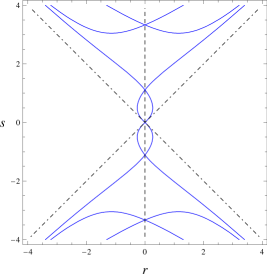
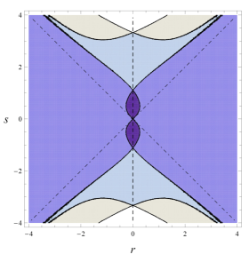
Figure 1: The figure on left shows the curves in the $az$-plane along which $H$ has spectral singularities. Here $r:=a\Re(z)$ and $s:=a\Im(z)$. The vertical dashed lines correspond to the $\mathcal{P}\mathcal{T}$-symmetric case with purely imaginary $z$. The diagonal lines are the lines $s=\pm r$. The figure on the right shows the number of bound states (generally complex eigenvalues with square-integrable eigenfunctions). As the color changes from the darkest to lightest the number of bound sates will changes from zero to four.

For small values of $|z|$ with $|\Re(z)|>|\Im(z)|$, $H$ has a bound state (an eigenvalue with a square-integrable eigenfunction). This corresponds to a real eigenvalue if and only if $|\Im(z)|=0$, [15]. In the darkest region shown in the right-hand figure the Hamiltonian is free of spectral singularities and bound states. This is a region where it is quasi-Hermitian, and (41) provides a reliable metric operator.

4.3 Equivalent Hermitian Hamiltonian

Inserting (42) in (3) and doing the necessary calculations, we obtain the following expression for the equivalent Hermitian operator $h$ defined by the metric operator (41).

$$h(x,y) = \delta(x-y)\left(-\frac{d^{2}}{dx^{2}}+\Re(z)\left[\delta(x^{-})-\delta(x^{+})\right]\right)$$ (47)

$$\begin{array}[]{c}+\mbox{\large$\frac{\Im(z)^{2}}{8}$}\Big{\{}\delta(x^{+})[\theta(y^{+})-\theta(y-3a)]+\delta(x^{-})[\theta(y+3a)-\theta(y^{-})]\\ \hskip 96.73918pt+\delta(y^{+})[\theta(x^{+})-\theta(x-3a)]+\delta(y^{-})[\theta(x+3a)-\theta(x^{-})]\Big{\}}+\mathcal{O}(z^{3}).\end{array}$$

If we multiply $h(x,y)$ by $\frac{\hbar^{2}}{2m\ell^{3}}$ and use (29), we obtain the dimensionful Hermitian Hamiltonian operator:

$$\mathbf{\mathrm{h}}({\rm x},{\rm y}) = \delta({\rm x}-{\rm y})\left(-\frac{\hbar^{2}}{2m}\frac{d^{2}}{d{\rm x}^{2}}+\Re(\zeta)\left[\delta({\rm x}-\alpha)-\delta({\rm x}+\alpha)\right]\right)$$ (51)

$$\begin{array}[]{cc}&+\mbox{\large$\frac{m\Im(\zeta)^{2}}{4\hbar^{2}}$}\Big{\{}\delta({\rm x}+\alpha)[\theta({\rm y}+\alpha)-\theta({\rm y}-3\alpha)]+\delta({\rm x}-\alpha)[\theta({\rm y}+3\alpha)-\theta({\rm y}-\alpha)]\\ &\hskip 102.43008pt+\delta({\rm y}+\alpha)[\theta({\rm x}+\alpha)-\theta({\rm x}-3\alpha)]+\delta({\rm y}-\alpha)[\theta({\rm x}+3\alpha)-\theta({\rm x}-\alpha)]\Big{\}}+\mathcal{O}(\zeta^{3}),\end{array}$$

where $\zeta=\zeta_{+}=\frac{\hbar^{2}z}{2m\ell}$. The second order (nonlocal) part of the Hamiltonian (51) is equivalent to the anti-Hermitian part of the Hamiltonian (30). In the following we study the effect of this nonlocal part on the energy expectation value, ${\rm E}_{\psi}:=\langle\psi|\mathbf{\mathrm{h}}|\psi\rangle$, for a particle described by a normalized Gaussian position wave function $\psi\in L^{2}(\mathbb{R})$.

The action of $\mathbf{\mathrm{h}}$ on an arbitrary element $\psi$ of the Hilbert space $\mathcal{H}$ is given by

$$\langle{\rm x}|\mathbf{\mathrm{h}}|\psi\rangle = -\frac{\hbar^{2}}{2m}\psi^{\prime\prime}({\rm x})+\Re(\zeta)\left[\delta({\rm x}-\alpha)\psi(\alpha)-\delta({\rm x}+\alpha)\psi(-\alpha)\right]$$

$$+\frac{m[\Im(\zeta)]^{2}}{4\hbar^{2}}\Big{\{}[\theta({\rm x}+\alpha)-\theta({\rm x}-3\alpha)]\psi(-\alpha)+[\theta({\rm x}+3\alpha)-\theta({\rm x}-\alpha)]\psi(\alpha)$$

$$\hskip 56.9055pt+\delta({\rm x}+\alpha)\int_{-\alpha}^{3\alpha}\psi({\rm y})d{\rm y}+\delta({\rm x}-\alpha)\int_{-3\alpha}^{\alpha}\psi({\rm y})d{\rm y}\Big{\}}+\mathcal{O}(\zeta^{3}).$$

The first line of this Equation coincides with the action of the Hermitian part of the original quasi-Hermitian Hamiltonian, namely $\mathbf{\mathrm{H}}_{h.}=\mathbf{\mathrm{H}}^{(0)}+\mathbf{\mathrm{H}}^{(1)}_{h.}$.

In view of (4.3),

$${\rm E}_{\psi}:=\langle\psi|\mathbf{\mathrm{h}}|\psi\rangle = \frac{\hbar^{2}}{2m}\int_{-\infty}^{\infty}|\psi^{\prime}({\rm x})|^{2}d{\rm x}+\Re(\zeta)\left[|\psi(\alpha)|^{2}-|\psi(-\alpha)|^{2}\right]$$

$$+\frac{m[\Im(\zeta)]^{2}}{2\hbar^{2}}~{}\Re\left(\psi^{*}(-\alpha)\int_{-\alpha}^{3\alpha}\psi({\rm x})d{\rm x}+\psi^{*}(\alpha)\int_{-3\alpha}^{\alpha}\psi({\rm x})d{\rm x}\right)+\mathcal{O}(\zeta^{3}),$$

where $\psi$ is a normalized wave function. A typical example is a Gaussian wave packet,

$$\psi_{1}({\rm x})=\frac{1}{(\pi\sigma^{2})^{1/4}}\exp\left(-\frac{{\rm x}^{2}}{2\sigma^{2}}+ik{\rm x}\right),$$ (54)

with mean position $\langle{\rm x}\rangle_{\psi_{1}}:=\langle\psi_{1}|{\rm x}|\psi_{1}\rangle=0$ and mean momentum $\langle{\rm p}\rangle_{\psi_{1}}:=\langle\psi_{1}|{\rm p}|\psi_{1}\rangle=\hbar k$. Substituting (54) in (4.3), we find

$${\rm E}_{\psi_{1}}=\frac{\hbar^{2}}{4m}\left(2k^{2}-\sigma^{-2}\right)+\frac{m[\Im(\zeta)]^{2}}{\sqrt{2}\hbar^{2}}\>U(\alpha,\sigma,k)+\mathcal{O}(\zeta^{3}),$$ (55)

where

$$U(\alpha,\sigma,k):=\exp\left(-\frac{\alpha^{2}+k^{2}\sigma^{4}}{2\sigma^{2}}\right)\Re\left\{e^{-ik\alpha}\left[{\rm erf}\left(\frac{ik\sigma^{2}+3\alpha}{\sqrt{2}\sigma}\right)-{\rm erf}\left(\frac{ik\sigma^{2}-\alpha}{\sqrt{2}\sigma}\right)\right]\right\}$$ (56)

describes the effect of the nonlocal part of $\mathbf{\mathrm{h}}$ (equivalently the non-Hermitian part of $\mathbf{\mathrm{H}}$), and ${\rm erf}({\rm x}):=\frac{2}{\sqrt{\pi}}\int_{0}^{\rm x}e^{-t^{2}}dt$ is the error function.

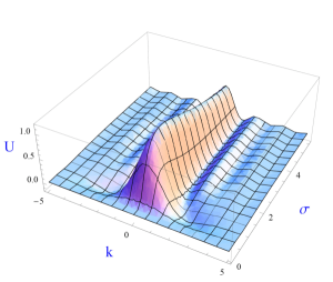
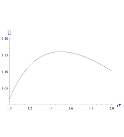
Figure 2: Plots of $U(1,\sigma,k)$ (on the left) and $U(1,\sigma,0)$ (on the right).

Figure 2 shows the plots of $U(\alpha,\sigma,k)$ and $U(\alpha,\sigma,0)$ for $\alpha=1$. It turns out that the non-Hermiticity effect attains its maximum around $(\sigma,k)=(1.5\alpha,0)$ and decays rapidly for the mean momentums $\langle{\rm p}\rangle_{\psi_{1}}=\hbar k$ outside the range $\left(-\frac{\hbar}{\alpha},\frac{\hbar}{\alpha}\right)$.

Next, we compute the energy expectation value for a stationary Gaussian wave packet with mean position $\langle{\rm x}\rangle_{\psi_{2}}={\rm x}_{0}$:

$$\psi_{2}({\rm x})=\frac{1}{(\pi\sigma^{2})^{1/4}}\exp\left(-\frac{({\rm x}-{\rm x}_{0})^{2}}{2\sigma^{2}}\right).$$ (57)

In view of (4.3), we have

$$E_{\psi_{2}} = \frac{\hbar^{2}}{4m\sigma^{2}}+\frac{\Re[\zeta]}{\sigma\sqrt{\pi}}V(\alpha,\sigma,{\rm x}_{0})+\frac{m[\Im(\zeta)]^{2}}{2\sqrt{2}\hbar^{2}}W(\alpha,\sigma,{\rm x}_{0})+\mathcal{O}(\zeta^{3}),$$ (58)

$$V(\alpha,\sigma,{\rm x}_{0}) := \exp\left(-\sigma^{-2}({\rm x}_{0}-\alpha)^{2}\right)-\exp\left(-\sigma^{-2}({\rm x}_{0}+\alpha)^{2}\right)$$ (59)

$$W(\alpha,\sigma,{\rm x}_{0}) := \exp\left({-\frac{(\alpha+{\rm x}_{0})^{2}}{2\sigma^{2}}}\right)\left\{{\rm erf}\left(\frac{\alpha+{\rm x}_{0}}{\sqrt{2}\sigma}\right)+{\rm erf}\left(\frac{3\alpha-{\rm x}_{0}}{\sqrt{2}\sigma}\right)\right.$$

$$\hskip 105.2751pt+\left.e^{\frac{2\alpha{\rm x}_{0}}{\sigma^{2}}}\left[{\rm erf}\left(\frac{\alpha-{\rm x}_{0}}{\sqrt{2}\sigma}\right)+{\rm erf}\left(\frac{3\alpha+{\rm x}_{0}}{\sqrt{2}\sigma}\right)\right]\right\}.$$

Here $W(\alpha,\sigma,{\rm x}_{0})$ reflects the effect of the nonlocal part of $\mathbf{\mathrm{h}}$ (non-Hermitian part of $\mathbf{\mathrm{H}}$).

Figure 3 shows the plots of $W(1,\sigma,{\rm x}_{0})$ for $\sigma\in[0.03,0.6]$ and $\sigma\in[0.2,10]$. The non-Hermitian effect attains its maximum at $({\rm x}_{0}\approx 0,\sigma\approx 1.5\alpha)$. For small values of $\sigma$, it persists for wave packets with mean position belonging to open intervals $(\pm\alpha-1.5\sigma,\pm\alpha+1.5\sigma)$. Outside these intervals it decays rapidly.

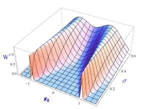
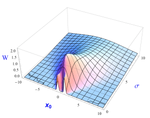
Figure 3: Plots of $W(\alpha,\sigma,{\rm x}_{0})$ for $\sigma\in[0.03,0.6]$ (on the left) and $\sigma\in[0.2,10]$ (on the right) in units where $\alpha=1$.

4.4 Pseudo-Hermitian Position and Momentum Operators

To calculate the dimensionless pseudo-Hermitian position and momentum operators corresponding to the metric operator (41)-(42), we substitute $x$ and $p$ for $o$ in (27) and use $Q^{(1)}=-\eta^{(1)}$ and the identities:

$$\langle x|[x,A]|y\rangle=(x-y)\langle x|A|y\rangle,~{}~{}~{}~{}\langle x|[p,A]|y\rangle=-i(\partial_{x}-\partial_{y})\langle x|A|y\rangle,$$

where $A$ is a linear operator. This yields

$$\langle x|X|y\rangle = \langle x|x|y\rangle+\frac{i\Im(z)}{4}|x-y|\left[\theta(x^{+}+y^{+})-\theta(x^{-}+y^{-})\right]+\mathcal{O}(z^{2}),$$ (61)

$$\langle x|P|y\rangle = \langle x|p|y\rangle+\Im(z)\delta(x-y)\left[\theta(x^{+})-\theta(x^{-})\right]+\mathcal{O}(z^{2}).$$ (62)

Next we obtain the dimensionful pseudo-Hermitian position (${\rm X}:=\ell X$) and momentum (${\rm P}:=\frac{\hbar}{\ell}P$) operators:

$$\langle{\rm x}|{\rm X}|{\rm y}\rangle = \langle{\rm x}|{\rm x}|{\rm y}\rangle+\frac{im\Im(\zeta)}{2\hbar^{2}}|{\rm x}-{\rm y}|\left[\theta({\rm x}+{\rm y}+2\alpha)-\theta({\rm x}+y-2\alpha)\right]+\mathcal{O}(\zeta^{2}),$$ (63)

$$\langle{\rm x}|{\rm P}|{\rm y}\rangle = \langle{\rm x}|{\rm p}|{\rm y}\rangle+\frac{2m\Im(\zeta)}{\hbar}\delta({\rm x}-{\rm y})\left[\theta({\rm x}+\alpha)-\theta({\rm x}-\alpha)\right]+\mathcal{O}(\zeta^{2}).$$ (64)

4.5 Calculating Metric for More General Cases

In Section 4.2, we constructed a metric operator with the desired Hermitian limit for the cases that the coupling constants $\zeta_{\pm}$ differed by a sign. Our construction was based on the spectral method that yielded $\eta$ in terms of its spectral decomposition. An alternative method of constructing a metric operator for a Schrödinger operator, $-\frac{\hbar^{2}}{2m}\,\frac{d^{2}}{d{\rm x}^{2}}+v({\rm x})$, is the one based on the universal differential equation [33]:

$$\left(-\partial_{{\rm x}}^{2}+\partial_{{\rm y}}^{2}+\frac{2m}{\hbar^{2}}\left[v^{*}({\rm x})-v({\rm y})\right]\right)\eta({\rm x},{\rm y})=0.$$ (65)

In this section we use this method to extend the results of the preceding sections to a more general class of double-delta function potentials.

Consider a quasi-Hermitian Hamiltonian operator,

$$\mathbf{\mathrm{H}}_{1}=\mathbf{\mathrm{H}}^{(0)}+\mathbf{\mathrm{H}}^{(1)}_{a.h.}=-\frac{{\rm p}^{2}}{2m}+v_{1}({\rm x}),$$ (66)

with a purely imaginary potential $v_{1}=i\Im\left(v_{1}\right)$, and a corresponding metric operator $\eta_{1}$ satisfying (65) with $v=v_{1}$. Let $\zeta$ be a complex perturbation parameter such that $v_{1}$ is proportional to $\Im(\zeta)$. This suggests the following perturbative expansion for $\eta$.

$$\eta_{1}=1+\eta^{(1)}_{1}+\mathcal{O}(\zeta^{2}).$$ (67)

Next, suppose that the potential $v_{1}$ is supplemented with a real part $v_{2}$ that is proportional to $\Re(\zeta)$. Then it is easy to see that up to the first order of perturbation, $\eta_{1}$ satisfies (65) for the potential $v_{1}({\rm x})+v_{2}({\rm x})$, i.e., $\eta_{1}$ is a metric operator also for the Hamiltonian

$$\mathbf{\mathrm{H}}_{2}=\mathbf{\mathrm{H}}_{1}+\mathbf{\mathrm{H}}^{(1)}_{h.}=-\frac{{\rm p}^{2}}{2m}+v_{1}({\rm x})+v_{2}({\rm x}).$$ (68)

Furthermore, in light of (25), the equivalent Hermitian Hamiltonian for $\mathbf{\mathrm{H}}_{1}$ and $\mathbf{\mathrm{H}}_{2}$ are respectively given by

$$\mathbf{\mathrm{h}}_{1} = \mathbf{\mathrm{H}}^{(0)}-\frac{1}{4}[\mathbf{\mathrm{H}}^{(1)}_{a.h.},\eta^{(1)}_{1}]+\mathcal{O}(\zeta^{3})$$

$$\mathbf{\mathrm{h}}_{2} = \mathbf{\mathrm{H}}^{(0)}+\mathbf{\mathrm{H}}^{(1)}_{h.}-\frac{1}{4}[\mathbf{\mathrm{H}}^{(1)}_{a.h.},\eta^{(1)}_{1}]+\mathcal{O}(\zeta^{3})=\mathbf{\mathrm{h}}_{1}+\mathbf{\mathrm{H}}^{(1)}_{h.}+\mathcal{O}(\zeta^{3}).$$ (69)

Now, we confine our attention to the double-delta function potential. In Section 4.2, we constructed an appropriate metric operator, namely (41), for a double-delta function potential whose couplings differed by a sign. In view of the argument given in the preceding paragraph, it is also a valid metric operator for the more general case that the real part of the coupling constants are arbitrary (but small) and their imaginary part differ by a sign:

$$\mathbf{\mathrm{H}}=-\frac{{\rm p}^{2}}{2m}+\zeta_{+}\delta({\rm x}-\alpha)+\zeta_{-}\delta({\rm x}+\alpha),~{}~{}\Im(\zeta_{+})=-\Im(\zeta_{-}).$$ (70)

Another class of potentials that admit (41) as an appropriate metric operator is [27]:

$$v({\rm x})=-\xi\delta({\rm x})+i\lambda\left[\delta({\rm x}-\alpha)-\delta({\rm x}+\alpha)\right],~{}~{}~{}~{}~{}\xi\in\mathbb{R}^{+},~{}~{}~{}\lambda\in\mathbb{R}.$$ (71)

Next, we use the metric operator (41) to compute the equivalent Hermitian Hamiltonian $\mathbf{\mathrm{h}}$ for the Hamiltonian (70). Using (69) and performing the necessary calculations, we find

$$\mathbf{\mathrm{h}}({\rm x},{\rm y}) = \delta({\rm x}-{\rm y})\left(-\frac{\hbar^{2}}{2m}\frac{d^{2}}{d{\rm x}^{2}}+\Re(\zeta_{+})\delta({\rm x}-\alpha)+\Re(\zeta_{-})\delta({\rm x}+\alpha)\right)$$ (75)

$$\begin{array}[]{cc}&+\frac{m[\Im(\zeta_{+})]^{2}}{4\hbar^{2}}\Big{\{}\delta({\rm x}+\alpha)[\theta({\rm y}+\alpha)-\theta({\rm y}-3\alpha)]+\delta({\rm x}-\alpha)[\theta({\rm y}+3\alpha)-\theta({\rm y}-\alpha)]\\ &\hskip 102.43008pt+\delta({\rm y}+\alpha)[\theta({\rm x}+\alpha)-\theta({\rm x}-3\alpha)]+\delta({\rm y}-\alpha)[\theta({\rm x}+3\alpha)-\theta({\rm x}-\alpha)]\Big{\}}+\mathcal{O}(\zeta^{3}).\end{array}$$

As we expected the nonlocal part of $\mathbf{\mathrm{h}}$ is identical with the one obtained for the special case where coupling constants differ by a sign.

The general $\mathcal{P}\mathcal{T}$-symmetric double-delta function potential ($\zeta_{+}=\zeta_{-}^{*}=:\zeta$) corresponds to a special case of the Hamiltonian (70). Our analysis shows that, within the framework of perturbation theory, the physical effects associated with the non-Hermiticity of the Hamiltonian $\mathbf{\mathrm{H}}$, that are contained in the nonlocal part of the equivalent Hermitian Hamiltonian $\mathbf{\mathrm{h}}$, are not sensitive to the presence of $\mathcal{P}\mathcal{T}$-symmetry. This is because by perturbing the Hermitian part of the Hamiltonian we may destroy its $\mathcal{P}\mathcal{T}$-symmetry while preserving the same non-Hermitian (nonlocal) effects on the physically observables quantities like energy expectation values.

Finally, we wish to stress that the above calculations of the metric operator and the equivalent Hermitian Hamiltonian are reliable only within the regions in the space of coupling constants that the Hamiltonian does not posses spectral singularities or bound states with complex eigenvalues. In Figure 4 we give the location of the spectral singularities and the number of bound sates for the general $\mathcal{P}\mathcal{T}$-symmetric case. In the region painted by the darkest color in the $r$-$s$-plane (where $r:=\frac{2am\ell}{\hbar^{2}}\Re(\zeta)$, $s:=\frac{2am\ell}{\hbar^{2}}\Im(\zeta)$) the Hamiltonian has no spectral singularities or bound states. Hence in this region it is quasi-Hermitian, and (41) gives a reliable metric operator provided that we stay within the part of this region that is close to the origin.

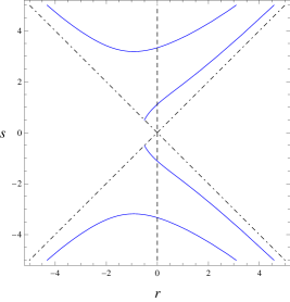
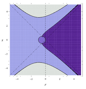
Figure 4: The curves along which the ${\mathcal{P}\mathcal{T}}$-symmetric Hamiltonian (70) with $\zeta_{+}=\zeta_{-}^{*}=:\zeta$ has spectral singularities (the figure on the left) and the number of bound states with (the figure on the right). As color changes from the darkest to the lightest, the number of bound sates takes the values $0,1,2,4$, respectively. The vertical dashed lines correspond to the purely imaginary coupling $\zeta$, and the diagonal (dotted-dashed) lines are the lines $r=\pm s$. There is a bound state within the circle $(r+1/2)^{2}+s^{2}=1/4$.

5 Concluding Remarks

In this article we have employed the pseudo-Hermitian formulation of quantum mechanics to study a quantum system defined by a Hamiltonian with two complex point interactions, $\mathbf{\mathrm{H}}={\rm p}^{2}/2m+\zeta_{-}\delta({\rm x}+\alpha)+\zeta_{+}\delta({\rm x}-\alpha)$. This requires the construction of an appropriate metric operator that reveals the structure of the physical Hilbert space and also the observables of the theory. It further allows for the construction of an equivalent Hermitian Hamiltonian operator.

The main difficulty one encounters in trying to construct a metric operator for $H$ is that depending on the choice of the eigenfunctions of $H^{\dagger}$, one obtains a “metric operator” that may be ill-defined or unbounded. In this article we could successfully construct a densely-defined and bounded metric operator to the first order of perturbation for the special cases that the coupling constants $\zeta_{\pm}$ differed by a sign. We use this metric operator to compute the corresponding equivalent Hermitian operator. This in turn allowed us to compute energy expectation values for a class of Gaussian wave packets. We then investigated the physical consequences of the non-Hermiticity of the Hamiltonian $H$ by examining the contribution of the anti-Hermitian part of the Hamiltonian (equivalently the nonlocal part of the equivalent Hermitian Hamiltonian) to the energy expectation values.

In view of the fact that the integral kernel of the metric operator is a solution of a certain differential equation, we could generalize our results to the cases that only the imaginary part of the coupling constants differed by a sign. This allowed for the application of our results for a general class of double-delta function potentials that included all $\mathcal{P}\mathcal{T}$-symmetric double-delta function potentials as a subclass. Our investigation of the physical effects of non-Hermiticity shows that (to the first nontrivial order of perturbation theory) these effects are not directly sensitive to the presence of $\mathcal{P}\mathcal{T}$-symmetry. This is because we can easily perturb the real part of the potential in such a way that the effects of non-Hermiticity is left unaltered while $\mathcal{P}\mathcal{T}$-symmetry is destroyed. Note however that if such a perturbation does not violate the quasi-Hermiticity of the Hamiltonian, the Hamiltonian will necessarily possess a symmetry that similarly to the $\mathcal{P}\mathcal{T}$-symmetry is generated by an invertible antilinear operator [13, 30]. This symmetry cannot however be interpreted as the space-time reflection symmetry.

Appendix A: Another Choice for the Wight Functions

If $\left|\frac{\Im(z_{\pm})}{\Re(z_{\pm})}\right|\ll 1$, and $\Re(z_{\pm})>0$, the Hamiltonian (30) is a quasi-Hermitian operator [15], and we can use $\epsilon_{\pm}:=\frac{\Im(z_{\pm})}{\Re(z_{\pm})}$ as perturbation parameters for a perturbative calculation of a metric operator. This requires selecting an appropriate set of $|{\phi}_{\mathfrak{a},k}^{\vec{z}}\rangle$ that would lead to a densely-defined bounded metric operator. A natural candidate is the following direct generalization of the expression obtained for a delta function potential with a complex coupling constant [31].

$$|{\phi}_{\mathfrak{a},k}^{\vec{z}}\rangle=u(z_{+},z_{-};k)|\psi_{\mathfrak{a},k}^{\vec{z^{*}}}\rangle,~{}~{}~{}~{}u(z_{+},z_{-};k):=\left(1+\frac{z_{+}z_{-}}{\gamma^{2}k^{2}}\right)^{-\frac{1}{2}},$$ (76)

where $\gamma\in\mathbb{R}^{+}$ is arbitrary and $|\psi_{\mathfrak{a},k}^{\vec{z^{*}}}\rangle$ are given in (33) - (34).

In view of (6), (34) and (76),

$$\eta(x,y)=\int_{-\infty}^{\infty}{\psi}_{1,k}^{\vec{z}^{*}}(x)\left({\psi}_{1,k}^{\vec{z}^{*}}(y)\right)^{*}W(z_{+},z_{-},k)dk,~{}~{}~{}~{}W(z_{+},z_{-},k):=|u(z_{+},z_{-},k)|^{2}.$$ (77)

Introducing $\kappa:=\frac{\gamma k}{\sqrt{r_{+}r_{-}}}:=\rho k$, $\varepsilon_{1}:=\epsilon_{+}+\epsilon_{-}$, and $\varepsilon_{2}:=\epsilon_{+}\epsilon_{-}$, we can expand $W=W(z_{+},z_{-},k)=W\left(r_{+}(1+i\epsilon_{+}),r_{-}(1+i\epsilon_{-}),\frac{\kappa}{\rho}\right)$ in powers of $\epsilon$:

$$W=\frac{\kappa^{2}}{1+\kappa^{2}}\left\{1-\frac{2\varepsilon_{2}}{1+\kappa^{2}}+\frac{{\varepsilon}_{1}^{2}+{\varepsilon}_{2}^{2}}{\left(1+\kappa^{2}\right)^{2}}\right\}^{-\frac{1}{2}}=\frac{\kappa^{2}}{1+\kappa^{2}}\left\{1+\frac{\varepsilon_{2}}{1+\kappa^{2}}-\frac{{\varepsilon}_{1}^{2}}{2\left(1+\kappa^{2}\right)^{2}}\right\}+\mathcal{O}(\epsilon^{4}).$$ (78)

Employing this relation in (77) and performing the necessary calculations, we find

$$\eta(x,y) = \eta_{0,0}(x,y)+\eta_{+,+}(x,y)+\eta_{-,-}(x,y)$$ (79)

$$+\eta_{+}(x,y)+\eta_{-}(x,y)+\eta_{-,+}(x,y)+(x\leftrightarrow y)^{*}+\mathcal{O}(\epsilon^{4}),$$

where

$$\eta_{0,0}(x,y)=\frac{1}{2\rho}~{}\vec{\mathcal{E}}.~{}\vec{\mathcal{I}}^{0}\left(\frac{x-y}{\rho}\right),$$ (80)

$$\eta_{\pm,\pm}(x,y)=\frac{\rho}{4}~{}r_{\pm}^{2}(1+\epsilon_{\pm}^{2})\theta(\pm x^{\mp})\theta(\pm y^{\mp})~{}\vec{\mathcal{E}}.~{}\left[\vec{\mathcal{I}}^{2}\left(\frac{x-y}{\rho}\right)-\vec{\mathcal{I}}^{2}\left(\frac{x^{\mp}+y^{\mp}}{\rho}\right)\right],$$ (81)

$$\eta_{\pm}(x,y)=\pm\frac{r_{\pm}(1+i\epsilon_{\pm})}{2}\theta(\pm y^{\mp})~{}\vec{\mathcal{E}}.~{}\left[\vec{\mathcal{I}}^{1}\left(\frac{x-y}{\rho}\right)-\vec{\mathcal{I}}^{1}\left(\frac{x^{\mp}+y^{\mp}}{\rho}\right)\right],$$ (82)

$$\eta_{-,+}(x,y)=\pm\frac{\gamma^{2}}{4\rho}\theta(y^{-})\theta(-x^{+})(1+\varepsilon_{2}+i(\epsilon_{+}-\epsilon_{-}))\times$$

$$~{}\vec{\mathcal{E}}.~{}\left[\vec{\mathcal{I}}^{2}\left(\frac{x^{+}+y^{+}}{\rho}\right)+\vec{\mathcal{I}}^{2}\left(\frac{x^{-}+y^{-}}{\rho}\right)-\vec{\mathcal{I}}^{2}\left(\frac{x-y}{\rho}\right)-\vec{\mathcal{I}}^{2}\left(\frac{x-y+4a}{\rho}\right)\right],$$ (83)

$$\vec{\mathcal{E}}:=(1,\varepsilon_{2},-\frac{\varepsilon_{1}^{2}}{2})=(1,\epsilon_{+}\epsilon_{-},-\frac{(\epsilon_{+}+\epsilon_{-})^{2}}{2}),~{}~{}~{}~{}\vec{\mathcal{I}}^{n}:=(\mathcal{I}_{n,1},\mathcal{I}_{n,2},\mathcal{I}_{n,3}),~{}~{}~{}~{}n=0,1,2,$$ (84)

$$\mathcal{I}_{n,m}(\alpha):=\frac{1}{2\pi}\int_{-\infty}^{\infty}\frac{k^{2-n}e^{ik\alpha}}{(1+k^{2})^{m}}~{}dk,~{}~{}~{}~{}~{}~{}\vec{\mathcal{I}}_{m}:=(\mathcal{I}_{0,m}~{},~{}\mathcal{I}_{1,m}~{},~{}\mathcal{I}_{2,m}),~{}~{}~{}~{}m\geq 1,~{}~{}~{}~{}~{}~{}$$ (85)

$$\vec{\mathcal{I}}_{1}=\left(\delta(\alpha)-\frac{e^{-|\alpha|}}{2}~{},~{}\frac{ie^{-|\alpha|}}{2}{\rm sign}(\alpha)~{},~{}\frac{e^{-|\alpha|}}{2}\right),~{}~{}~{}~{}~{}~{}\vec{\mathcal{I}}_{2}=\frac{e^{-|\alpha|}}{4}\left(1-|\alpha|~{},~{}i\alpha~{},~{}1+|\alpha|\right),$$ (86)

$$\vec{\mathcal{I}}_{3}=\frac{e^{-|\alpha|}}{16}\Big{(}1+|\alpha|-\alpha^{2}~{},~{}i\alpha(1+|\alpha|)~{},~{}3(1+|\alpha|)+\alpha^{2}\Big{)},$$ (87)

$x^{\pm}$ and $y^{\pm}$ are given by (43), and $\left(x\leftrightarrow y\right)$ stands for the sum of the previous terms with $x$ and $y$ interchanged.

It is not difficult to see that $\vec{\mathcal{E}}=(1,0,0)+\mathcal{O}(\epsilon^{2})$ and $\vec{\mathcal{E}}\cdot\vec{\mathcal{I}}^{n}=\mathcal{I}_{n,1}+\mathcal{O}(\epsilon^{2})$. Inserting the values of $\mathcal{I}_{n,1}$ given by (86) - (87) in (80) - (83) and rearranging the terms, we have

$$\eta(x,y) = \frac{1}{2}\delta(x-y)$$ (88)

$$+e^{-\frac{|x-y|}{\rho}}\Big{\{}\frac{-1}{4\rho}+\frac{\rho}{8}[r_{+}^{2}\theta(x^{-})\theta(y^{-})+r_{-}^{2}\theta(-x^{+})\theta(-y^{+})]-\frac{\gamma^{2}}{8\rho}\theta(-x^{+})\theta(y^{-})(1+i\epsilon_{+}-i\epsilon_{-})$$

$$\hskip 51.21504pt+\frac{ir_{+}}{4}\theta(y^{-}){\rm sign}(x-y)(1+i\epsilon_{+})-\frac{ir_{-}}{4}\theta(-y^{+}){\rm sign}(x-y)(1+i\epsilon_{-})\Big{\}}$$

$$+{e^{-\frac{|x^{-}+y^{-}|}{\rho}}}\Big{\{}-\frac{\rho}{8}r_{+}^{2}\theta(x^{-})\theta(y^{-})+\frac{\gamma^{2}}{8\rho}\theta(-x^{+})\theta(y^{-})(1+i\epsilon_{+}-i\epsilon_{-})$$

$$\hskip 65.44142pt-\frac{ir_{+}}{4}\theta(y^{-}){\rm sign}(x^{-}+y^{-})(1+i\epsilon_{+})\Big{\}}$$

$$+{e^{-\frac{|x^{+}+y^{+}|}{\rho}}}\Big{\{}-\frac{\rho}{8}r_{-}^{2}\theta(-x^{+})\theta(-y^{+})+\frac{\gamma^{2}}{8\rho}\theta(-x^{+})\theta(y^{-})(1+i\epsilon_{+}-i\epsilon_{-})$$

$$\hskip 65.44142pt-\frac{ir_{-}}{4}\theta(-y^{+}){\rm sign}(x^{+}+y^{+})(1+i\epsilon_{-})\Big{\}}$$

$$-{e^{-\frac{|x-y+4a|}{\rho}}}\Big{\{}\frac{\gamma^{2}}{8\rho}\theta(-x^{+})\theta(y^{-})(1+i\epsilon_{+}-i\epsilon_{-})\Big{\}}$$

$$+(x\leftrightarrow y)^{*}+\mathcal{O}(\epsilon^{2}).$$

As suggested by this relation, $\eta$ is actually densely-defined and (perturbatively) bounded, but in the Hermitian limit it does not tend to the identity operator.

Appendix B: A Proper Choice for the Wight Functions

One can check that unless one fixes $u_{\pm,\mathfrak{b}}(k)$ in a very special way the metric operator corresponding to (38) is an unbounded operator. In order to obtain such a special choice we consider the ansatz:

$${\phi}_{1,k}^{\vec{z}}(x) = {\psi}_{1,k}^{\vec{z^{*}}}(x)+{\phi}_{1,k}^{\mathfrak{v}}(x)+\mathcal{O}(z^{2}),$$ (89)

$${\phi}_{2,k}^{\vec{z}}(x) = {\phi}_{1,-k}^{\vec{z}}(x),$$ (90)

where ${\psi}_{\mathfrak{a},k}^{\vec{z^{*}}}(x)$ are given by Eqs. (33) - (34),

$${\phi}_{1,k}^{\mathfrak{v}}(x) := \frac{i}{k}\sum_{\lambda=\pm}\sum_{j=1}^{m}e^{-ib_{j}k}z_{\lambda}^{*}\left(v_{j,1,\lambda}^{*}{\psi}_{1,k}^{\vec{z^{*}}}(x)+v_{j,2,\lambda}^{*}{\psi}_{2,k}^{\vec{z^{*}}}(x)\right)+\mathcal{O}(z^{2})$$ (91)

$$= \frac{i}{{\sqrt{2\pi}}}\sum_{\lambda=\pm}\sum_{j=1}^{m}\frac{z_{\lambda}^{*}}{k}\left(v_{j,1,\lambda}^{*}e^{-ik(b_{j}-x)}+v_{j,2,\lambda}^{*}e^{-ik(b_{j}+x)}\right)+\mathcal{O}(z^{2}),$$

$m$ is a positive integer, and $b_{j}$ and $v_{j,\mathfrak{b},\lambda}$ are respectively real and complex free coefficients. By defining $\mu(\mathfrak{b}):=2\mathfrak{b}-3$, we can rewrite ${\phi}_{1,k}^{\mathfrak{v}}(x)$ in a more compact form, namely

$${\phi}_{1,k}^{\mathfrak{v}}(x)=\frac{1}{\sqrt{2\pi}}\sum_{\lambda=\pm}\sum_{\mathfrak{b}=1}^{2}\sum_{j=1}^{m}\frac{iz_{\lambda}^{*}v_{j,\mathfrak{b},\lambda}^{*}}{k}e^{-ik[b_{j}+\mu(\mathfrak{b})x]}+\mathcal{O}(z^{2}).$$ (92)

For the cases where (90) holds, we can use (6) to express $\eta(x,y)=\langle x|\eta|y\rangle$ as

$$\eta(x,y)=\int_{-\infty}^{\infty}{\phi}_{1,k}^{\vec{z}}(x)\left({\phi}_{1,k}^{\vec{z}}(y)\right)^{*}dk.$$ (93)

Using

$$\frac{1}{i\pi}\int_{-\infty}^{\infty}\frac{e^{ik\alpha}}{k}\>dk={\rm sign}(\alpha),~{}~{}~{}~{}\frac{1}{2\pi}\int_{-\infty}^{\infty}e^{ik\alpha}\,dk=\delta(\alpha),$$ (94)

and (89) - (93), we then find

$$\eta(x,y)=\delta(x-y)+\eta^{(1)}(x,y)+\mathcal{O}(z^{2}),$$ (95)

where

$$\eta^{(1)}(x,y) := \eta^{(1)}_{+}(x,y)+\eta^{(1)}_{-}(x,y)+\eta^{(1)}_{\mathfrak{v}}(x,y)+\left(x\leftrightarrow y\right)^{*},$$ (96)

$$\eta^{(1)}_{+}(x,y) := \frac{z_{+}}{4}\left\{{\rm sign}(x+y-2a)-{\rm sign}(x-y)\right\}\theta(y-a),$$ (97)

$$\eta^{(1)}_{-}(x,y) := -\frac{z_{-}}{4}\left\{{\rm sign}(x+y+2a)-{\rm sign}(x-y)\right\}\theta(-y-a),$$ (98)

$$\eta^{(1)}_{\mathfrak{v}}(x,y) := \sum_{\lambda=\pm}\sum_{\mathfrak{b}=1}^{2}\sum_{j=1}^{m}\eta^{(1)}_{j,\mathfrak{b},\lambda}(x,y)=\sum_{\lambda=\pm}\sum_{\mathfrak{b}=1}^{2}\sum_{j=1}^{m}\frac{z_{\lambda}v_{j,\mathfrak{b},\lambda}}{2}{\rm sign}(x+\mu(\mathfrak{b})y+b_{j}).$$ (99)

Note that $\eta^{(1)}_{\mathfrak{v}}(x,y)$ depends on our choice of the free coefficients $v_{j,\mathfrak{b},\lambda}$ and $b_{j}$ in (92). Our aim is to make a choice that would lead to a an appropriate metric operator.

First, we use the identity

$${\rm sign}(u+v)[{\rm sign}(u)+{\rm sign}(v)]=1+{\rm sign}(u){\rm sign}(v),$$ (100)

to obtain

$$\eta_{+}^{(1)}(x,y) = \frac{z_{+}}{8}[-2{\rm sign}(x-y)-{\rm sign}(x^{-}+y^{-})+1]+\frac{z_{+}}{4}{\rm sign}(x-y)\theta(-x^{-}-y^{-})$$ (101)

$$= \frac{z_{+}}{8}[{\rm sign}(x^{-}+y^{-})+1]-\frac{z_{+}}{4}{\rm sign}(x-y)\theta(x^{-}+y^{-}),$$

$$\eta_{-}^{(1)}(x,y) = \frac{z_{-}}{8}[2{\rm sign}(x-y)-{\rm sign}(x^{+}+y^{+})+1]-\frac{z_{-}}{4}{\rm sign}(x-y)\theta(x^{+}+y^{+}),$$ (102)

where $x^{\pm}$ and $y^{\pm}$ are given by Eq. (43).

Next, we rewrite ${\phi}_{1,k}^{\mathfrak{v}}(x)$ in the form

$${\phi}_{1,k}^{\mathfrak{v}}(x) = {\phi^{\prime}}_{1,k}^{\mathfrak{v}}(x)-\frac{i}{k\sqrt{2\pi}}\left[\frac{z^{*}_{+}}{4}{e^{-ik(x-2a)}}-\frac{z^{*}_{-}}{4}{e^{-ik(x+2a)}}+\frac{z^{*}_{-}}{2}{e^{ikx}}\right],$$ (103)

where

$${\phi^{\prime}}_{1,k}^{\mathfrak{v}}(x) := \frac{1}{\sqrt{2\pi}}\sum_{\lambda=\pm}\sum_{\mathfrak{b}=1}^{2}\sum_{j=1}^{m^{\prime}}\frac{iz_{\lambda}^{*}v_{j,\mathfrak{b},\lambda}^{*}}{k}e^{-ik(b_{j}+\mu(\mathfrak{b})x)},$$

and $m^{\prime}$ is a positive integer. Using the above equations, the first order term $\eta^{(1)}(x,y)$ of $\eta(x,y)$ can be rewritten as

$$\eta^{(1)}(x,y) = {\eta^{\prime}}^{(1)}_{+}(x,y)+{\eta^{\prime}}^{(1)}_{-}(x,y)+{\eta^{\prime}}^{(1)}_{\mathfrak{v}}(x,y)+\left(x\leftrightarrow y\right)^{*},$$ (104)

$${\eta^{\prime}}^{(1)}_{\pm}(x,y) = \frac{z_{\pm}}{8}[1-2{\rm sign}(x-y)\theta(x^{\mp}+y^{\mp})],$$ (105)

$${\eta^{\prime}}^{(1)}_{\mathfrak{v}}(x,y) = \sum_{\lambda=\pm}\sum_{\mathfrak{b}=1}^{2}\sum_{j=1}^{m^{\prime}}\eta^{(1)}_{j,\mathfrak{b},\lambda}(x,y)=\sum_{\lambda=\pm}\sum_{\mathfrak{b}=1}^{2}\sum_{j=1}^{m^{\prime}}\frac{z_{\lambda}v_{j,\mathfrak{b},\lambda}}{2}{\rm sign}(x+\mu(\mathfrak{b})y+b_{j})$$

$$= {\eta}^{(1)}_{\mathfrak{v}}(x,y)+\frac{z_{+}}{8}{\rm sign}(x^{-}+y^{-})-\frac{z_{-}}{8}{\rm sign}(x^{+}+y^{+})+\frac{z_{-}}{4}{\rm sign}(x-y).$$

Setting ${\phi^{\prime}}_{1,k}^{\mathfrak{v}}(x)=0$ or equally ${\eta^{\prime}}^{(1)}_{\mathfrak{v}}(x,y)=0$ yields

$${\eta^{\prime}}^{(1)}(x,y)={\eta^{\prime}}^{(1)}_{+}(x,y)+{\eta^{\prime}}^{(1)}_{-}(x,y)+(x\leftrightarrow y)^{*},$$ (107)

which is generally not a bounded operator. But if we confine our attention to the special case where $z_{+}=-z_{-}=:z$, we find

$${\eta^{\prime}}^{(1)}(x,y)=\frac{i\Im(z)}{2}{\rm sign}(x-y)[\theta(x^{+}+y^{+})-\theta(x^{-}+y^{-})],$$ (108)

which is a bounded operator [6].

References

- [1] C. M. Bender and S. Boettecher, Phys. Rev. Lett. 80, 5243 (1998).
- [2] A. Ruschhaupt, F. Delgado, and J. G. Muga, J. Phys. A 38, L171 (2005).
- [3] A. Mostafazadeh, Phys. Rev. Lett. 102, 220402 (2009).
- [4] S. Klaiman, U. Günther, and N. Moiseyev, Phys. Rev. Lett. 101, 080402 (2008).
- [5] Z. Ahmed, J. Phys. A 42, 472005 (2009).
- [6] A. Batal, Application of Pseudo-Hermitian Theory to the -symmetric Delta-Function Potential with Continuous Real Spectrum, Koç University, M.Sci. thesis, 2007.
- [7] C. M. Bender, S. Boettecher, and P. N. Meisinger, J. Math. Phys. 40, 2201 (1999).
-
[8]
Z. H. Musslimani, K. G. Makris, R. El-Ganainy, and
D. N. Christodoulides, Phys. Rev. Lett. 100, 103904 (2008);
K. G. Makris, R. El-Ganainy, D.N. Christodoulides, and Z. H. Musslimani, Phys. Rev. Lett. 100, 103904 (2008). - [9] C. M. Bender, Rep. Prog. Phys. 70, 947 (2007).
- [10] A. Mostafazadeh, “Pseudo-Hermitian Quantum Mechanics,” preprint ArXiv: 0810.5643.
- [11] A. Mostafazadeh, J. Math. Phys. 43, 205 (2002).
- [12] A. Mostafazadeh, J. Math. Phys. 43, 2814 (2002).
- [13] A. Mostafazadeh, J. Math. Phys. 43, 3944 (2002).
- [14] F. G. Scholtz, H. B. Geyer, and F. J. W. Hahne, Ann. Phys. (NY) 213 74 (1992).
- [15] A. Mostafazadeh and H. Mehri-Dehnavi, J. Phys. A 42, 125303 (2009).
-
[16]
W. D. Heiss, Phys. Rep. 242, 443 (1994);
E. Narevicius and N. Moiseyev, Phys. Rev. Lett. 81, 2221 (1998); 84, 1681 (2000);
M. V. Berry, J. Mod. Opt. 50, 63 (2003); Czech. J. Phys. 54, 1039 (2004);
A. A. Mailybaev, O. N. Kirillov, and A. P. Seyranian, Phys. Rev. A 72, 014104 (2005);
M. Müller and I. Rotter, J. Phys. A 41, 244018 (2008);
H. Mehri-Dehnavi and A. Mostafazadeh, J. Math. Phys. 49, 082105 (2008);
D. Viennot, J. Math. Phys. 50, 052101 (2009). -
[17]
C. Dembowski, H.-D. Gräf, H. L. Harney,
A. Heine, W. D. Heiss, H. Rehfeld, and A. Richter, Phys. Rev. Lett. 86, 787 (2001);
C. Dembowski, B. Dietz, H.-D. Gräf, H. L. Harney, A. Heine, W. D. Heiss, and A. Richter, Phys. Rev. E 69, 056216 (2004);
T. Stehmann, W. D. Heiss, and F. G. Scholtz, J. Phys. A 37, 7813 (2004);
S.-B. Lee, J. Yang, S. Moon, S.-Y. Lee, J.-B. shim, S. W. Kim, J.-H. Lee, and K. An, Phys. Rev. Lett. 103, 134101 (2009);
H. Cartarius, J. Main, and G. Wunner, Phys. Rev. Lett. 99, 173003 (2007). - [18] G. Sh. Guseinov, Pramana, J. Phys. 73, 587 (2009).
- [19] A. Mostafazadeh, Phys. Rev. A 80, 032711 (2009).
- [20] A. Mostafazadeh and A. Batal, J. Phys. A 37, 11645 (2004).
- [21] A. Mostafazadeh, J. Phys. A 36, 7081 (2003).
- [22] A. Mostafazadeh, J. Phys. A 41, 244017 (2008).
- [23] A. Mostafazadeh, J. Phys. A 38, 6557 (2005).
- [24] A. Mostafazadeh, J. Phys. A 39, 10171 (2006).
-
[25]
C. M. Bender, D. C. Brody, and H.F. Jones, Phys. Rev. D 70, 025001 (2004);
C. M. Bender and H.F. Jones, Phys. Lett. A 328, 102 (2004). -
[26]
H. F. Jones, Phys. Lett. A 262, 242
(1999);
Z. Ahmed, Phys. Lett. A 286, 231 (2001);
S. Albeverio, A.-M. Fei, and P. Kurasov, Lett. Math. Phys. 59, 227 (2002);
J. M. Cerveró and A. Rodríguez, J. Phys. A 37, 10167 (2004);
H. Uncu and E. Demiralp, Phys. Lett. A 359, 190 (2006);
F. A. B. Coutinho, Y. Nogami, and F. M. Toyama, J. Phys. A 41, 235306 (2008);
S. Albeverio, U. Günther, and S. Kuzhel, J. Phys. A 42, 105205 (2009). - [27] H. F. Jones, Phys. Rev. D 78, 065032 (2008).
-
[28]
H. F. Jones, Phys. Rev. D 76, 125003
(2007);
M. Znojil, Phys. Rev. D 80, 045009 (2009). - [29] A. Mostafazadeh, Class. Quantum. Grav. 20, 155 (2003); J. Math. Phys. 46, 102108 (2005).
- [30] A. Mostafazadeh, J. Math. Phys. 44, 947 (2003); Nucl. Phys. B 640, 419 (2002).
- [31] A. Mostafazadeh, J. Phys. A 39, 13495 (2006).
- [32] C. Figueira de Morisson Faria and A. Fring, J. Phys. A 39, 9269 (2006).
- [33] A. Mostafazadeh, J. Math. Phys. 47, 072103 (2006).