Abstract

Electromagnetic waves, solving the full set of Maxwell equations in vacuum, are numerically computed. These waves occupy a fixed bounded region of the three dimensional space, topologically equivalent to a toroid. Thus, their fluid dynamics analogs are vortex rings. An analysis of the shape of the sections of the rings, depending on the angular speed of rotation and the major diameter, is carried out. Successively, spherical electromagnetic vortex rings of Hill’s type are taken into consideration. For some interesting peculiar configurations, explicit numerical solutions are exhibited.

Keywords: Electromagnetism; Solitary wave; Optimal set; Toroid; Hill’s vortex.

PACS Nos.: 41.20.Jb; 47.32.Ef; 02.70.Dh

Published in the International Journal of Modern Physics C, Vol. 21, No. 1 (2010), pp. 11-32. DOI: 10.1142/S0129183110014926

1 Introduction

We start by recalling that the classical set of Maxwell equations in vacuum has the form:

$$\frac{\partial{\bf E}}{\partial t}~{}=~{}c^{2}{\rm curl}{\bf B}$$ (1)

$${\rm div}{\bf E}~{}=~{}0$$ (2)

$$\frac{\partial{\bf B}}{\partial t}~{}=~{}-{\rm curl}{\bf E}$$ (3)

$${\rm div}{\bf B}~{}=~{}0$$ (4)

where $c$ is the speed of light and the two fields ${\bf E}$ and $c{\bf B}$ have the same dimensions.

It is customary to introduce the potentials ${\bf A}$ and $\Phi$ such that:

$${\bf B}~{}=~{}\frac{1}{c}~{}{\rm curl}{\bf A}~{}~{}~{}~{}~{}~{}~{}~{}~{}{\bf E}~{}=~{}-\frac{1}{c}\frac{\partial{\bf A}}{\partial t}~{}-~{}\nabla\Phi$$ (5)

By this assumption, equations (3) and (4) are automatically satisfied. In addition, we require that the vector and the scalar potentials are related by the following Lorenz gauge condition:

$${\rm div}{\bf A}~{}+~{}\frac{1}{c}\frac{\partial\Phi}{\partial t}~{}=~{}0$$ (6)

Furthermore, one can deduce the two wave equations:

$$\frac{\partial^{2}{\bf A}}{\partial t^{2}}~{}-~{}c^{2}\Delta{\bf A}~{}=~{}0$$ (7)

$$\frac{\partial^{2}\Phi}{\partial t^{2}}~{}-~{}c^{2}\Delta\Phi~{}=~{}0$$ (8)

We are concerned with studying, from the numerical viewpoint, the development of a solitary electromagnetic wave, trapped in a bounded region of space having a toroid shape. In the cylindrical case (equivalent to a 2-D problem), and partly for 3-D problems, this analysis was proposed and carried out in Ref. [1]. There, the goal was to simulate stable elementary subatomic particles by means of rotating photons. Here, we would like to continue the discussion of the 3-D case, because the subject might be of more general interest. Since exact solutions are only available in special situations, we shall make use of finite element techniques to approximate the model equations. In order to determine solutions of the vector wave equation, confined in appropriate steady domains, we will perform an in-depth analysis of the lower spectrum of a suitable elliptic operator, in dependance of the shape and magnitude of the regions. In particular, we will be concerned with those domains realizing the coincidence of the fourth and the fifth eigenvalues of the differential operator. The reasons for this choice will become clear to the reader as we proceed with the investigation.

The structures we consider in this paper display a strong analogy with fluid dynamics vortex rings (see for instance Ref. [2], [3], [4]). For this reason, the techniques we apply here may be useful to get additional results in the study of the development of fluid vortices. As a matter of fact, peculiar configurations are going to be presented and discussed, opening the path to an interesting scenario for future extensions.

2 The Cylindrical Case

Let us quickly review the results obtained in Ref. [1], concerning waves rotating around the axis of a cylinder. The magnetic field is oriented in the same direction as the $z$-axis, so that the electric field lays on the orthogonal plane. The variables are expressed in cylindrical coordinates $(r,z,\phi)$. The solutions, however, will not depend on $z$.

Several options are examined in Ref. [1], here we show the most significant one, that will be used later to construct the toroid case. We denote by $\omega$ a positive parameter which characterizes the frequency of rotation of the wave: $\nu=c\omega/\pi$. Up to multiplicative constant, the two vector fields are given by:

$${\bf E}=\left(\frac{2J_{2}(\omega r)}{\omega r}\cos(c\omega t-2\phi),~{}~{}0,~{}~{}J_{2}^{\prime}(\omega r)\sin(c\omega t-2\phi)\right)$$

$${\bf B}~{}=~{}\frac{1}{c}\Big{(}0,~{}~{}J_{2}(\omega r)\cos(c\omega t-2\phi),~{}~{}0\Big{)}$$ (9)

for $0\leq\phi<2\pi$, $0\leq r\leq\delta_{0}/\omega~{}$ and any $z$. The fields in (9) are defined on a disk of radius $\delta_{0}/\omega$, whose size is inversely proportional to the angular speed of rotation. In Ref. [1] , figure 5.7, the reader can see the displacement of the electric field for $t=0$ (some on-line animations can be viewed in Ref. [5], rotating photons).

In (9) we find the Bessel function $J_{k}$ (see, e.g., Ref. [6]) that solves the following differential equation:

$$J_{k}^{\prime\prime}(x)~{}+~{}\frac{J_{k}^{\prime}(x)}{x}~{}-~{}\frac{k^{2}J_{k}(x)}{x^{2}}~{}+~{}J_{k}(x)~{}=~{}0$$ (10)

It is also useful to recall that Bessel functions are connected by the relations:

$$J_{k}^{\prime}(x)~{}+~{}\frac{kJ_{k}(x)}{x}~{}=~{}J_{k-1}(x)$$ (11)

$$J_{k+1}(x)~{}=~{}\frac{2kJ_{k}(x)}{x}~{}-~{}J_{k-1}(x)$$ (12)

The quantity $~{}\delta_{0}\approx 5.135622~{}$ turns out to be the first zero of $J_{2}$. In this way, for $r=\delta_{0}/\omega$, the components $E_{1}$ and $B_{2}$ are zero. Note also that ${\bf E}$ and ${\bf B}$ vanish for $r=0$, since $J_{k}(x)$ decays as $x^{k}$ for $x\rightarrow 0$. The choice $k=1$ is not permitted because it does not allow to prolong with continuity the fields up to $r=0$, although, one could take into consideration solutions for $k$ integer greater than 2:

$${\bf E}=\left(\frac{kJ_{k}(\omega r)}{\omega r}\cos(c\omega t-k\phi),~{}~{}0,~{}~{}J_{k}^{\prime}(\omega r)\sin(c\omega t-k\phi)\right)$$

$${\bf B}~{}=~{}\frac{1}{c}\Big{(}0,~{}~{}J_{k}(\omega r)\cos(c\omega t-k\phi),~{}~{}0\Big{)}$$ (13)

The idea is to simulate a $k$-body rotating system in equilibrium. This somehow explains why the case $k=1$ is not going to produce meaningful solutions.

For $k=2$, the electromagnetic fields in (9) are generated by the following potentials:

$${\bf A}~{}=~{}-\frac{1}{\omega}\Big{(}J_{3}(\omega r)\sin(c\omega t-2\phi),~{}~{}0~{},~{}~{}J_{3}(\omega r)\cos(c\omega t-2\phi)\Big{)}$$

$$\Phi~{}=~{}-\frac{1}{\omega}J_{2}(\omega r)\cos(c\omega t-2\phi)$$

satisfying the Lorenz condition (6) and the equations (7)-(8). The reader can check this by direct differentiation. We observe that $A_{1}$ and $A_{3}$ have a phase difference of 45 degrees, since: $~{}\sin(c\omega t-2\phi)=\cos(c\omega t-2(\phi+\pi/4))$. Denoting by $a(r)=J_{3}(\omega r)$ the term depending only on the radial variable, we easily discover that (see (10) for $k=3$):

$$-\left(\frac{d^{2}}{dr^{2}}+\frac{1}{r}\frac{d}{dr}-\frac{9}{r^{2}}\right)a~{}=~{}\omega^{2}a$$ (14)

We can introduce a new function $w=\frac{d}{dr}a+\frac{3}{r}a$. A straightforward computation, using relation (14) and its derivative, brings to:

$$-\left(\frac{d^{2}}{dr^{2}}+\frac{1}{r}\frac{d}{dr}-\frac{4}{r^{2}}\right)w~{}=~{}-\left(a^{\prime\prime\prime}+\frac{a^{\prime\prime}}{r}-\frac{10a^{\prime}}{r^{2}}+\frac{18a}{r^{3}}\right)$$

$$-~{}\frac{3}{r}\left(a^{\prime\prime}+\frac{a^{\prime}}{r}-\frac{9a}{r^{2}}\right)~{}=~{}\omega^{2}\left(a^{\prime}+\frac{3a}{r}\right)~{}=~{}\omega^{2}w$$ (15)

By scaling the interval in order to impose the boundary conditions $w(0)=0$ and $w(1)=0$, the eigenvalue problem (15) takes the form:

$$Lw~{}=~{}-\left(\frac{d^{2}}{dr^{2}}+\frac{1}{r}\frac{d}{dr}-\frac{4}{r^{2}}\right)w~{}=~{}\delta_{0}^{2}w$$ (16)

where $L$ is a positive-definite differential operator. Such an operator is the same as the one we would obtain from the Laplacian, after separation of variables in polar coordinates, by imposing homogeneous Dirichlet boundary conditions on a disk $\Omega$ (on the plane $(r,\phi)$) of radius equal to 1. In this circumstance, the eigenvalue:

$$\lambda~{}=~{}\delta_{0}^{2}~{}\approx~{}26.37461$$ (17)

has double multiplicity. The corresponding eigenfunctions are orthogonal in $L^{2}(\Omega)$ and show a phase difference of 45 degrees (see figures 1 and 2).

$$\begin{array}[]{|c|c|}\hline\cr~{}~{}~{}~{}~{}~{}~{}\lambda{}{}{}{}{}{}{}&{\it multiplicity}\\ \hline\cr~{}~{}5.78318&1\\ 14.68197&2\\ 26.37461&2\\ 30.47126&1\\ 40.70646&2\\ 49.21845&2\\ 57.58294&2\\ 70.84999&2\\ \hline\cr\end{array}$$

Table 1: Eigenvalues counted with their multiplicity of the Laplacian on a disk of radius 1, with homogeneous Dirichlet boundary conditions.

In other words, by computing the spectrum of the Laplacian on a disk of radius 1 (see table 1), the one given in (17) is the common eigenvalue of the fourth and the fifth eigenfunctions. Note that there are no eigenvalues with multiplicity greater than 2. We also note that $\Phi=0$ at the boundary of $\Omega$. These simple observations will be of primary importance in the discussion to follow.

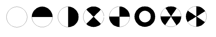
Figure 1: Signature of the first 8 eigenfunctions of the Laplace’s equation on a disk. The first eigenfunction ($w_{1}$) does not change sign. The two successive ones ($w_{2}$ and $w_{3}$) display a phase difference of 90 degrees. Then, we have $w_{4}$ and $w_{5}$ with a phase difference of 45 degrees. The next one ($w_{6}$) is a single multiplicity eigenfunction, while the last ones ($w_{7}$ and $w_{8}$) have a phase difference of 30 degrees.

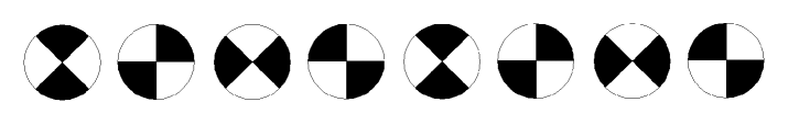
Figure 2: Solutions of the wave equation on a disk are obtained by linearly combining independent eigenfunction having the same eigenvalue. For example, a complete rotation is simulated through the sequence: $w_{4},w_{5},-w_{4},-w_{5},w_{4},w_{5},-w_{4},-w_{5}$. Intermediate situations are obtained by taking $w_{4}\cos ct\sqrt{\lambda}+w_{5}\sin ct\sqrt{\lambda}$, with $0\leq ct\sqrt{\lambda}\leq 2\pi$, where $\lambda$ is the common eigenvalue.

3 The Toroid Case

We are ready to study the 3-D case. In cylindrical coordinates $(r,z,\phi)$, we consider the potentials:

$${\bf A}~{}=~{}\frac{1}{c}\Big{(}a(t,r,z),~{}b(t,r,z),~{}0\Big{)}~{}~{}~{}~{}~{}~{}\Phi~{}=~{}-\left(\frac{\partial A}{\partial r}+\frac{A}{r}+\frac{\partial B}{\partial z}\right)$$ (18)

where $a$ and $b$ are functions to be computed, while $A$ and $B$ are their primitives with respect to the time variable. In this context, the Lorenz condition (6) turns out to be automatically satisfied. The functions $a$ and $b$ will describe the time evolution, in a certain region $\Omega$ of the plane $(r,z)$, of a rotating wave similar to the one studied in the previous section (differently from the previous case, $\Omega$ is now vertically oriented). Since there is no dependance on $\phi$, the solution is automatically extended to a toroid $\Sigma$, having section $\Omega$, with the axis parallel to the $z$-axis.

From the potentials we deduce the electromagnetic fields (see (5)):

$${\bf E}~{}=~{}\Big{(}-\frac{\partial\Phi}{\partial r}-\frac{1}{c^{2}}\frac{\partial a}{\partial t},~{}-\frac{\partial\Phi}{\partial z}-\frac{1}{c^{2}}\frac{\partial b}{\partial t},~{}0\Big{)}~{}~{}~{}~{}~{}~{}~{}~{}~{}{\bf B}~{}=~{}\frac{1}{c^{2}}\Big{(}0,~{}0,~{}\frac{\partial b}{\partial r}-\frac{\partial a}{\partial z}\Big{)}$$ (19)

We now require ${\bf E}$ and ${\bf B}$ to satisfy the whole set of Maxwell equations (in alternative, we get the same conclusions by imposing (7) and (8)). The result is the following system:

$$\frac{1}{c^{2}}\frac{\partial^{2}a}{\partial t^{2}}~{}=~{}\frac{\partial^{2}a}{\partial z^{2}}~{}+~{}\frac{\partial}{\partial r}\left(\frac{\partial a}{\partial r}~{}+~{}\frac{a}{r}\right)$$ (20)

$$\frac{1}{c^{2}}\frac{\partial^{2}b}{\partial t^{2}}~{}=~{}\frac{\partial^{2}b}{\partial z^{2}}~{}+~{}\frac{\partial^{2}b}{\partial r^{2}}~{}+~{}\frac{1}{r}\frac{\partial b}{\partial r}$$ (21)

We can couple $a$ and $b$ through the boundary condition:

$$\frac{\partial a}{\partial z}~{}=~{}\frac{\partial b}{\partial r}$$ (22)

which amounts to ask $~{}{\bf B}=c^{-1}{\rm curl}{\bf A}=0~{}$ at the contour of $\Omega$. The field ${\bf E}$ is tangential to the same boundary. As a matter of fact, thanks to (18)-(20)-(21), one can write:

$${\bf E}~{}=~{}\left(\frac{\partial}{\partial z}\Big{(}\frac{\partial A}{\partial z}-\frac{\partial B}{\partial r}\Big{)},~{}-\frac{1}{r}\frac{\partial}{\partial r}\Big{(}r\frac{\partial A}{\partial z}-r\frac{\partial B}{\partial r}\Big{)},~{}0\right)$$ (23)

which means that ${\bf E}$ is orthogonal to the gradient of $~{}r\Big{(}\frac{\partial}{\partial z}A-\frac{\partial}{\partial r}B\Big{)}$. Since (22) is valid for any $t$, such a gradient is orthogonal to the boundary of $\Omega$, showing that ${\bf E}$ is tangential.

Note that now the set $\Omega$ is not going to be a circle. As done in Ref. [1], section 5.4, we set $~{}y=r-\eta$. The domain $\Omega$ will be centered at the point $(\eta,0)$, where $\eta>0$ is large enough to avoid intersection of $\Omega$ with the $z$-axis. The quantity $2\eta$ is related to the major diameter of the toroid.

By differentiating the first equation with respect to $z$ and the second one with respect to $y$, one gets:

$$\begin{cases}\displaystyle\frac{1}{c^{2}}\frac{\partial^{2}u}{\partial t^{2}}~{}=~{}\frac{\partial^{2}u}{\partial z^{2}}~{}+~{}\frac{\partial}{\partial y}\left(\frac{\partial u}{\partial y}+\frac{u}{y+\eta}\right)\\ \\ \displaystyle\frac{1}{c^{2}}\frac{\partial^{2}v}{\partial t^{2}}~{}=~{}\frac{\partial^{2}v}{\partial z^{2}}~{}+~{}\frac{\partial}{\partial y}\left(\frac{\partial v}{\partial y}+\frac{v}{y+\eta}\right)\end{cases}$$ (24)

where we took $u=\frac{\partial}{\partial z}a~{}$ and $~{}v=\frac{\partial}{\partial r}b=\frac{\partial}{\partial y}b$, with $u-v=0~{}$ on $\partial\Omega$. Furthermore, with the substitutions $~{}\tilde{u}=u\sqrt{y+\eta}$, $\tilde{v}=v\sqrt{y+\eta}$, one obtains:

$$\begin{cases}\displaystyle\frac{1}{c^{2}}\frac{\partial^{2}\tilde{u}}{\partial t^{2}}~{}=~{}\frac{\partial^{2}\tilde{u}}{\partial z^{2}}~{}+~{}\frac{\partial^{2}\tilde{u}}{\partial y^{2}}~{}-~{}\frac{3}{4}\frac{\tilde{u}}{(y+\eta)^{2}}\\ \\ \displaystyle\frac{1}{c^{2}}\frac{\partial^{2}\tilde{v}}{\partial t^{2}}~{}=~{}\frac{\partial^{2}\tilde{v}}{\partial z^{2}}~{}+~{}\frac{\partial^{2}\tilde{v}}{\partial y^{2}}~{}-~{}\frac{3}{4}\frac{\tilde{v}}{(y+\eta)^{2}}\end{cases}$$ (25)

to be solved in $\Omega$, with the boundary condition: $~{}\tilde{u}-\tilde{v}=0$.

Similarly to the case examined in section 2, we look for solutions associated to the second mode ($k=2$ in (13)) with respect to the angle of rotation. According to the captions of figures 1 and 2, the functions $\tilde{u}$ and $\tilde{v}$ should have a phase difference of 45 degrees (this property is now qualitative, since $\Omega$ is not a perfect disk). We fix the area of $\Omega$ to be equal to $\pi$. For $\eta$ tending to infinity, the set $\Omega$ converges to a circle of radius 1 and the electromagnetic fields coincide with those given in (9) for $\omega=\delta_{0}$.

We proceed by introducing a new unknown $w=\tilde{u}-\tilde{v}$ and by taking the difference of the two equations in (25). Then, we can get rid of the time variable and pass to the stationary eigenvalue problem:

$$\begin{cases}\displaystyle Lw~{}=~{}-~{}\frac{\partial^{2}w}{\partial z^{2}}~{}-~{}\frac{\partial^{2}w}{\partial y^{2}}~{}+~{}\frac{3}{4}\frac{w}{(y+\eta)^{2}}~{}=~{}\lambda w~{}~{}~{}~{}{\rm in}~{}\Omega\\ \displaystyle w~{}=~{}0~{}~{}~{}~{}~{}~{}~{}{\rm on}~{}\partial\Omega\end{cases}$$ (26)

Thus, we would like $\lambda>0$ to be an eigenvalue of the positive-definite differential operator: $L=-\frac{\partial^{2}}{\partial z^{2}}-\frac{\partial^{2}}{\partial y^{2}}+\frac{3}{4}(y+\eta)^{-2}$, with homogeneous Dirichlet boundary conditions. In addition, since we want two independent eigenfunctions with a difference of phase of 45 degrees, the multiplicity of $\lambda$ must be equal to 2. This implicitly defines $\Omega$. More precisely, we require that $\lambda=\lambda_{4}=\lambda_{5}$, where $\lambda_{4}$ and $\lambda_{5}$ are the eigenvalues of the fourth and the fifth eigenfunctions, $w_{4}$ and $w_{5}$, of $L$ on $\Omega$. In order to preserve energy, these eigenfunctions will be normalized in $L^{2}(\Omega)$. In this way, by setting:

$$\tilde{u}(t,y,z)-\tilde{v}(t,y,z)~{}=~{}w_{4}(y,z)\sin(ct\sqrt{\lambda})~{}+~{}w_{5}(y,z)\cos(ct\sqrt{\lambda})$$ (27)

one gets a full solution of the system (25). We can finally recover the electromagnetic fields by the expressions (see (23)):

$${\bf E}=\frac{1}{c\sqrt{\lambda}}\left(\frac{\partial}{\partial z}\Big{(}\frac{-w_{4}\cos\zeta+w_{5}\sin\zeta}{\sqrt{y+\eta}}\Big{)},~{}~{}~{}~{}~{}~{}~{}~{}~{}~{}~{}~{}~{}~{}\right.$$

$$\left.~{}~{}~{}~{}~{}~{}~{}~{}~{}~{}~{}~{}~{}~{}~{}~{}~{}~{}~{}\frac{-1}{\sqrt{y+\eta}}\frac{\partial}{\partial y}\Big{(}(-w_{4}\cos\zeta+w_{5}\sin\zeta)\sqrt{y+\eta}\Big{)},~{}0\right)$$

$${\bf B}~{}=~{}\frac{1}{c^{2}}\left(0,~{}~{}0,~{}~{}\frac{w_{4}\sin\zeta+w_{5}\cos\zeta}{\sqrt{y+\eta}}\right)$$ (28)

with $\zeta=ct\sqrt{\lambda}$. As in figure 2, by varying the parameter $t$, we can simulate a rotating object.

Of course, we could also take into consideration the case $k>2$ (see the 2-D analog (13)) by studying the behavior of eigenvalues with higher magnitude. The search, in this case, should be addressed to the determination of couples of independent eigenfunctions sharing the same eigenvalue. We think this is a viable option, although, in order to maintain the discussion at a simple level, we will not analyze this extension.

We now define $\Sigma=\Omega\times[0,2\pi[$, in order to get a 3-D solution not depending on $\phi$. In fluid dynamics this structure is known as vortex ring (see for instance Ref. [2], section 7.2, or  [3]). On the surface of $\Sigma$, field ${\bf E}$ is tangential and ${\bf B}$ is zero. At every point inside $\Sigma$, the time average during a period of oscillation, of both ${\bf E}$ and ${\bf B}$, is zero (see the animations in Ref. [5]).

We would like to know more about the shape of $\Sigma$. Considering that not all the sets $\Omega$ are such that $\lambda_{4}$ and $\lambda_{5}$ are equal, we can use this property in order to determine the right domain. This problem admits however infinite solutions. In the next section we discuss how to find numerically some suitable configurations.

4 On the Optimal Shape of $\Omega$

We first observe that, among the sets with fixed area equal to $\pi$, the circle of radius 1, minimizes the eigenvalues of the Laplacian with homogeneous Dirichlet boundary conditions (see for instance Ref. [7]). Due to symmetry arguments, all the eigenvalues related to the angular modes have multiplicity 2 (see table 1 and figure 1). The eigenfunctions are supposed to be orthogonal and normalized in $L^{2}(\Omega)$. Then, the normal derivative of the eigenfunction related to the lowest eigenvalue, has constant value on the boundary of the disk. Similarly, the sum of the squares of the normal derivatives of the eigenfunctions related to the second and the third eigenvalues, is constant along the boundary. The same is true for all the couples of eigenfunctions relative to other eigenvalues with double multiplicity (the fourth and the fifth, for example).

We now replace the Laplacian by the new elliptic operator $L=-\frac{\partial^{2}}{\partial z^{2}}-\frac{\partial^{2}}{\partial y^{2}}+\frac{3}{4}(y+\eta)^{-2}$ (see (26)), with homogeneous Dirichlet boundary conditions. We are concerned with finding a set $\Omega$, with area equal to $\pi$, such that the fourth and the fifth eigenvalues, $\lambda_{4}$ and $\lambda_{5}$, of $L$ are coincident. Thanks to (27), this allows us to determine solutions of a wave-type equation, rotating inside $\Omega$ with an angular velocity proportional to $\sqrt{\lambda}$, where $\lambda=\lambda_{4}=\lambda_{5}$. In table 2, we report the eigenvalues of $L$ on the disk centered in $(y,z)=(0,0)$ and radius equal to 1. If $~{}0<\eta<1~{}$ the differential operator is singular inside $\Omega$ (the corresponding toroid region $\Sigma$ has no central hole). Therefore, we take $\eta\geq 1$. The case $\eta=1$, where the axis $y=-\eta$ (or, equivalently, $r=0$) touches $\Omega$ at the boundary, is still admissible. The table shows the results for different values of $\eta$. For $\eta$ large, the fourth and the fifth eigenvalues are quite similar, due to the fact that the term $~{}\frac{3}{4}(y+\eta)^{-2}~{}$ becomes small. For $\eta$ close to 1, the situation is not too bad, anyway. This is especially true for the highest eigenvalues, since the corresponding eigenfunctions, due to the boundary constraints, decay faster near the border of $\Omega$. Therefore, they do not “feel” too much the presence of the term $~{}\frac{3}{4}(y+\eta)^{-2}$.

$$\begin{array}[]{|c|c|c|c|c|}\hline\cr&~{}~{}~{}~{}\eta=1{}{}{}{}{}&~{}~{}~{}~{}\eta=1.2{}{}{}{}&~{}~{}~{}~{}\eta=1.5{}{}{}{}&~{}~{}~{}~{}\eta=2{}{}{}{}{}\\ \hline\cr\lambda_{1}&~{}~{}6.90&~{}~{}6.46&~{}~{}6.18&~{}~{}5.99\\ \lambda_{2}&15.71&15.33&15.08&14.90\\ \lambda_{3}&16.75&15.68&15.19&14.93\\ \lambda_{4}&28.06&27.27&26.86&26.63\\ \lambda_{5}&28.36&27.35&26.88&26.64\\ \hline\cr\end{array}$$

Table 2: The first 5 eigenvalues of the operator $L$ on a disk of radius 1, for different values of $\eta$.

For any fixed $\eta$, we would like to adjust the shape of $\Omega$ with the help of some iterative procedure. The idea is to correct the boundary in order to fulfill a certain condition at the limit. Before getting some interesting answers (see later), we tried unsuccessfully different approaches. Let us discuss the one that looked more promising. We consider the substitution:

$$\hat{w}(y,z)~{}=~{}\frac{w(s,z)}{\sqrt{y+\eta}}~{}~{}~{}~{}~{}{\rm where}~{}~{}s=(y+\eta)^{2}$$ (29)

In this way (26) becomes:

$$\begin{cases}\displaystyle-\Big{(}4s~{}\frac{\partial^{2}\hat{w}}{\partial s^{2}}~{}+~{}\frac{\partial^{2}\hat{w}}{\partial z^{2}}\Big{)}~{}=~{}\lambda\hat{w}~{}~{}~{}~{}{\rm in}~{}\Omega\\ \\ \displaystyle\hat{w}~{}=~{}0~{}~{}~{}~{}~{}~{}~{}{\rm on}~{}\partial\Omega\end{cases}$$ (30)

where now the operator is a Laplacian with a variable coefficient. Concerning the operator $L_{\beta}=-\beta\frac{\partial^{2}}{\partial s^{2}}-\frac{\partial^{2}}{\partial z^{2}}$, for $\beta>0$ constant, the domain $\Omega$ of fixed area equal to $\pi$, optimizing the set of eigenvalues, is an ellipse. As in the case of the circle ($\beta=1$), we have infinite eigenvalues with double multiplicity. In addition, if $\hat{w}$ is the first eigenfunction of $L_{\beta}$, the following relation is easily checked:

$$\beta\Big{(}\frac{\partial\hat{w}}{\partial s}\Big{)}^{2}~{}+~{}\Big{(}\frac{\partial\hat{w}}{\partial z}\Big{)}^{2}~{}=~{}{\rm constant}~{}{\rm on}~{}\partial\Omega$$ (31)

The idea is to generalize the above relation in the case of variable coefficients. Hence, let us suppose that $\hat{w}$ is an eigenfunction corresponding to the first eigenvalue in (30), we may require that:

$$4s\Big{(}\frac{\partial\hat{w}}{\partial s}\Big{)}^{2}~{}+~{}\Big{(}\frac{\partial\hat{w}}{\partial z}\Big{)}^{2}~{}=~{}{\rm constant}~{}{\rm on}~{}\partial\Omega$$ (32)

For points where $s$ is large, we expect the curvature of the boundary of $\Omega$ to be high, and viceversa. The resulting $\Sigma$ is a kind of doughnut, a bit flattened on the internal side. Due to (29), in terms of $w$ one has:

$$(y+\eta)\left[\Big{(}\frac{w}{2\sqrt{y+\eta}}+\frac{\partial w}{\partial y}\Big{)}^{2}+\Big{(}\frac{\partial w}{\partial z}\Big{)}^{2}\right]$$

$$=~{}(y+\eta)\left[\Big{(}\frac{\partial w}{\partial y}\Big{)}^{2}+\Big{(}\frac{\partial w}{\partial z}\Big{)}^{2}\right]~{}=~{}{\rm constant}$$ (33)

where we used that $w=0$ on $\partial\Omega$.

Relation (33) is the “target” we would like to reach by implementing our iterative method. To this end, starting from the circle of radius 1, we compute the eigenfunction (normalized in $L^{2}(\Omega)$) corresponding to the lowest eigenvalue in (26). We then compute its normal derivatives on $\partial\Omega$ and correct $\Omega$ in order to enforce condition (33). For points belonging to the boundary, the updating procedure is performed as follows:

$${\bf P}_{\it new}~{}=~{}{\bf P}_{\it old}~{}+~{}\theta{\cal E}{\bf N}$$ (34)

where ${\bf N}$ is the outer normal derivative, $\theta$ is a relaxation parameter and ${\cal E}$ is the difference between the normal derivative evaluated in ${\bf P}_{\it old}$ and the average of the normal derivatives computed on the boundary of the current $\Omega$. After every correction, the area of $\Omega$ is set to $\pi$, with the help of a linear transformation. At the limit, we would like to have ${\cal E}=0$.

In order to compute eigenvalues and eigenfunctions we used a finite element code. In particular, we implemented MODULEF (see Ref. [8] and  [9]) with $P_{2}$ elements. The grid was fine enough to have reliable results up to the second decimal digit (at least for the first eigenvalue). The solver is based on a QR algorithm. The points to be updated through the iterative method (34) are the vertices of the triangles belonging to $\partial\Omega$. The normal derivative at these points is the average of the normal derivatives at the mid-points of the two sides of the contiguous triangles. After the entire boundary has been modified, a brand-new grid is generated in $\Omega$. The performances of this technique are far from being optimal, but their improvement is not in the scopes of the present paper.

Unfortunately, despite all the efforts, the method did not want to converge. A possible explanation is that relation (33) cannot be realized, because it is wrong from the theoretical viewpoint. The iterative technique (34) was however a good starting point to try successive variants, and, finally, we had success with the following scheme:

$${\bf P}_{\it new}~{}=~{}{\bf P}_{\it old}~{}+~{}\theta~{}|\lambda_{4}-\lambda_{5}|~{}\Big{(}n^{(y)},~{}~{}(y_{\it old}+\eta)n^{(z)}\Big{)}~{}~{}~{}~{}~{}{\rm on}~{}\partial\Omega$$ (35)

where ${\bf N}=(n^{(y)},n^{(z)})$ is again the outer normal derivative. This time, the fourth and the fifth eigenvalues of $L$ explicitly appear in the correcting term. Inspired by (33), the updating on the boundary is not uniform in the variable $y$, but the second component is weighted by the function $y+\eta$.

After suitably adjusting $\theta$, convergence is obtained in a few iterations. The result is a domain $\Omega$ yielding $\lambda_{4}=\lambda_{5}$. However, as anticipated, there are infinite other domains with this property. The most interesting ones should be those having a distribution of the eigenvalues as lower as possible, and making the shape of $\Omega$ as rounded as possible. We do not know if what we got by iterating (35) can be considered optimal with this respect. Nevertheless, it is important to have shown that the condition $\lambda_{4}=\lambda_{5}$ can be actually achieved (at least numerically). In table 3, one finds the modified eigenvalues for various $\eta$ (compare with table 2). Note instead that, for $\eta$ close to 1, $\lambda_{2}$ and $\lambda_{3}$ are not in good agreement.

For $\eta=1$ and $\eta=1.2$, the corresponding domains are displayed in figure 3. Even for $\eta$ close to 1, they are not too far from a circle. In figure 4, for $\eta=1$, we provide the plot of the fourth and the fifth eigenfunctions, actually showing a phase difference of 45 degrees (see also figures 1 and 2). For $\eta\geq 2$, $\Omega$ is practically a circle.

The analysis carried out in this section may help to understand the structure of fluid dynamics vortex rings. These are incredibly stable configurations, that have been widely studied, under different aspects. Among the vast literature we just mention for instance the papers:  [10], [11], [4], [12]. In addition, in Ref. [13], “optimal” sections of vortex rings are discussed. However, in the fluid dynamics case, the situations where the major diameter is relatively small, bring to more pronounced deformations of the sections.

$$\begin{array}[]{|c|c|c|c|c|}\hline\cr&~{}~{}~{}~{}\eta=1{}{}{}{}{}&~{}~{}~{}\eta=1.2{}{}{}{}{}&~{}~{}~{}\eta=1.5{}{}{}{}{}&~{}~{}~{}~{}\eta=2{}{}{}{}{}\\ \hline\cr\lambda_{1}&~{}~{}6.85&~{}~{}6.44&~{}~{}6.17&5.98\\ \lambda_{2}&15.76&15.32&15.04&14.89\\ \lambda_{3}&16.59&15.64&15.18&14.90\\ \lambda_{4}&28.08&27.24&26.83&26.60\\ \lambda_{5}&28.08&27.24&26.83&26.60\\ \hline\cr\end{array}$$

Table 3: The first 5 eigenvalues of the operator $L$ on the modified domain, for different values of $\eta$.

We are not able to discuss the stability of our electromagnetic vortices. Theoretically, using the newfound 3-D solutions, one should build the corresponding electromagnetic stress tensor and put it on the right-hand side of Einstein’s equation, as illustrated in Ref. [1]. Then, one has to solve this nonlinear system in order to determine the metric tensor. Finally, one should check that the quasi-circular orbits ($\Omega$ is not a perfect circle) followed by the light rays are actually geodesics of such a space-time environment. Note that this study depends on the parameter $\omega$, connected to the speed of rotation of the wave. For $\omega$ large, the size of $\Omega$ is small and the frequency is high. We expect one or more situations of equilibrium, where the gravitational setting and the centrifugal effect of the spinning solitons are compensated. This would mean that only particular geometries are admitted, specifying exactly the shape and the size of the toroid regions.

           

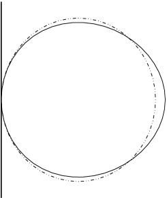
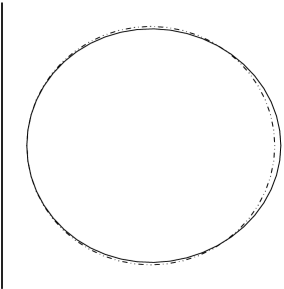
Figure 3: Toroid sections (solid line) compared to the circle of radius 1 (dashed-dotted line), for $\eta=1$ and $\eta=1.2$. The vertical line is the toroid axis of symmetry.

          

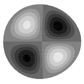
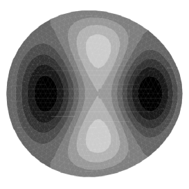
Figure 4: The forth and the fifth normalized eigenfunctions corresponding to the case $\eta=1$. Even if $\Omega$ is not a perfect circle, they actually display a phase difference of 45 degrees. Each eigenfunction has two positive (white) and two negative (black) bumps.

Of course, what we just said above turns out to be very hard to prove, both theoretically and computationally. Note that we are also omitting a stationary component of the electromagnetic fields, introduced in Ref. [1], which should provide charge and mass to the particle model. We do not insist further on this topic and we address the reader to Ref. [1] for additional information.

5 Hill’s Type Vortices

The next step is to examine what happens outside the spinning toroid. If we were dealing with a fluid vortex, due to viscosity, we might expect the formation of other external vortices developing at lower frequency. This circumstance can be observed in tornados or typhoons (see for instance Ref. [14]). In the theory presented in Ref. [1], an electromagnetic vortex, through a mechanism still to be clarified, captures the surrounding electromagnetic signals and generates a series of encapsulated shells vibrating with decreasing frequencies. These shells could be responsible for the quantum properties of matter.

           

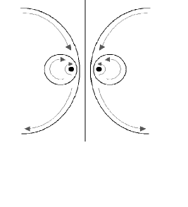
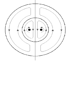
Figure 5: Successive layers of encapsulated vortex rings. In the first picture, the toroid regions have a common central hole. In the second one, the central hole is reduced to a vertical segment (Hill’s vortex). Of course, intermediate situations combining some shells of the first type, successively embedded in spherical vortices, could be taken into consideration.

Basically, there are two possible ways in which external ring vortices may develop. As the first picture of figure 5 shows, we may have a series of successive toroid structures, where all the fluid stream-lines pass through a common central hole. This situation is difficult to analyze, since we have no idea of the shape of these regions and the location of the primary vortex inside them. In practice, there are too many degrees of freedom to work with.

The other situation (second picture of figure 5) is more affordable. It represents an Hill’s spherical vortex (see Ref. [2], section 7.2, and Ref. [15] for some computational results), successively surrounded by other spherical layers. Thus, we now know exactly the shape of these structures. We just have to find the location (and the relative size) of the primary toroid vortex inside the most internal sphere. This research will lead us to interesting conclusions.

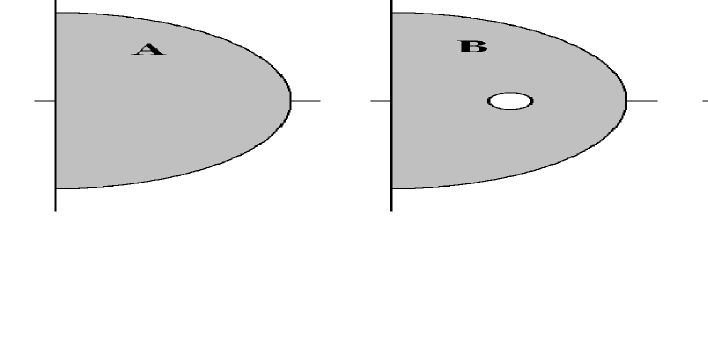
Figure 6: Sections of spherical vortices.

We start by considering the domain $A$ in figure 6. We set the radius equal to 1, so that the area is $\pi/2$. We solve in $\Omega=A$ the eigenvalue problem (26), involving the operator $L=-\frac{\partial^{2}}{\partial z^{2}}-\frac{\partial^{2}}{\partial r^{2}}+\frac{3}{4r^{2}}$ ($r=y+\eta$ with $\eta=0$). In the first column of table 4, we report the approximated eigenvalues, obtained by discretization with the finite element method. As the reader can notice, the fourth and the fifth eigenvalues are not coincident. Therefore, for a perfect spherical vortex, we have no chances to obtain solutions of the time-dependent wave equation. In alternative, we could modify a bit the shape of the domain $A$ or accept solutions whose stream-lines are not stationary. This is not however the path we would like to follow. If the rotation inside $\Omega$ is generated by an internal spinning toroid, we may cut out a hole (as in the domains $B$ and $C$) and see what happens to the spectrum of $L$. For simplicity, the hole will be a circle of a certain radius, suitably placed in a specific spot (although we know from section 4 that such a hole is slightly deformed). Playing with the size and the location of the circle, we look for situations in which the fourth and the fifth eigenvalues ($\lambda_{4}$ and $\lambda_{5}$) of $L$ are the same.

Surprisingly, this research seems to have a finite number of solutions. According to table 4 (columns 2 and 3), we have coincidence of $\lambda_{4}$ and $\lambda_{5}$ in two particular cases. In the first one, the center of the small circle is placed at point $(\frac{1}{2},0)$ and the radius is approximately equal to $r_{B}=.0505$. In the second one, the center is at $(\frac{1}{4},0)$ and the radius is approximately equal to $r_{C}=.00520$. With the exception of these cases, by varying the magnitude and the position of the internal circles, we always found $\lambda_{4}\not=\lambda_{5}$. In our experiments we did not try anyway all the possible configurations, thus we do not exclude the existence of other significant settings.

$$\begin{array}[]{|c|c|c|c|c|}\hline\cr&~{}{domain}~{}A{}&~{}{domain}~{}B{}&~{}{domain}~{}C{}&~{}{domain}~{}D{}\\ \hline\cr\lambda_{1}&20.24&30.23&21.64&0.63\\ \lambda_{2}&33.29&34.16&33.32&0.99\\ \lambda_{3}&48.94&54.82&49.09&1.45\\ \lambda_{4}&59.82&68.15&67.17&1.99\\ \lambda_{5}&67.11&68.15&67.17&1.99\\ \hline\cr\end{array}$$

Table 4: The first 5 eigenvalues of the operator $L$, based on the four domains given in figure 6, with homogeneous Dirichlet boundary conditions.

We provide in figure 7 the discretization grids. We show in figures 8 and 9, the time evolution of the rotating waves, obtained from expression (27) for equispaced values of $t$ with $c\sqrt{\lambda}t\in[0,\pi]$ (half-cycle). In the first case, the spherical flow is chained to the inner toroid. In the second case, the flow avoids the toroid, still remaining inside the spherical region. The sequence looks rather complicated. With the help of some imagination, one can see two anti-clockwise rotating waves, circulating independently in the lower and the upper quarters. They have different phases, so that the positive (white) bumps and the negative (black) ones, alternately merge to form a single protuberance situated near the center. The pictures only show half of the cycle. Then, the sequence restarts with the two colors interchanged. The corresponding animations can be found in Ref. [5] (click related papers).

We point out once again that we are dealing with electromagnetic waves. Therefore, we should ask ourselves what happens to the vector fields. Our plots actually show the evolution of the function $~{}\frac{\partial}{\partial r}b-\frac{\partial}{\partial z}a$, where ${\bf A}=c^{-1}(a,b,0)$ is the vector potential. Using (19), (23) and (28), one then computes ${\bf E}$ and ${\bf B}$. We discover that, at each point, when time passes, the tips of the arrows of the electric field turn around, describing elliptic orbits (see the animations in Ref. [5] in the case of a circle). The average of ${\bf E}$ during a cycle is zero. The frequency of rotation is globally the same, but, depending on the point, it is associated with a different phase, so that the general framework seems quite unorganized.

             

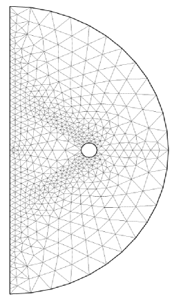
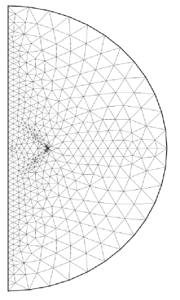
Figure 7: Discretization grids for the domains $B$ and $C$. The mesh is finer near the vertical axis since the differential operator $L$ is singular there. The degrees of freedom (internal and boundary nodes) are 2324 and 1968, respectively. In the right-hand side picture, the hole is very small.

     

     

     

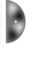
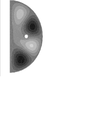
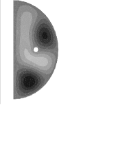
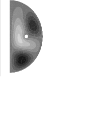
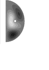
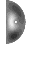
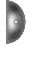
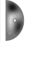
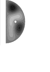
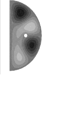
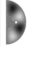
Figure 8: Rotating wave in a Hill’s spherical vortex: case of the domain $B$. The sequence is referred to half cycle and terminates with the colors inverted. The small inner circle is spinning at a frequency more than 12 times greater, dragging the spherical wave along circulating paths.

     

     

     

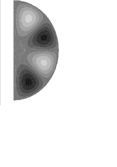
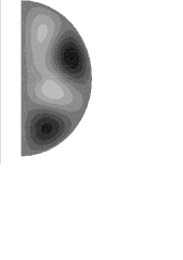
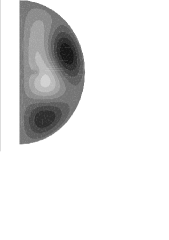
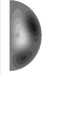
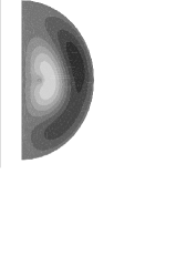
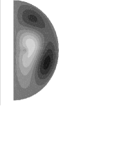
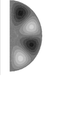
Figure 9: Rotating wave in a Hill’s spherical vortex: case of the domain $C$. The tiny inner circle (hardly visible in the pictures) is spinning at a frequency about 120 times greater. The behavior is qualitatively the same as in figure 8, but now the wave do not pass between the circle and the vertical axis.

From the size of the hole, we can estimate the frequency of rotation of the internal toroid regions. Such a frequency is proportional to the square root of a suitable eigenvalue. We take the value $\sqrt{26.37}\approx 5.135$, that, according to table 1, is the square root of the eigenvalue corresponding to the fourth and the fifth eigenfunctions, for a circle of radius 1. Afterwards, by scaling, we get the frequencies on the reduced circles: $5.135/r_{B}\approx 101.68$ and $5.135/r_{C}\approx 987.5$. Thus, the ratio between the frequencies of the inner spinning rings and the spherical vortices are given by (see table 4, the last line of the second and the third columns): $101.68/\sqrt{68.15}\approx 12.31$ and $987.5/\sqrt{67.17}\approx 120.48$, respectively. Note that these numbers may be affected by rounding errors (in particular, we expect an error bound of $\pm 0.005$ in the computation of the eigenvalues), therefore they should be taken with a little caution. Of course, more trustable results can be obtained with a finer mesh.

Finally, considering the second picture of figure 5, we can study the next external spherical shell, whose section is given by the set $D$ of figure 6. Let us suppose that the radius of the inner circumference is equal to 1, and let us find the outer radius $r_{D}$ in order to have $\lambda_{4}=\lambda_{5}$. From the experiments we deduce $r_{D}\approx 5.80$. This gives $\lambda_{4}=\lambda_{5}\approx 1.99$ (see the last column of table 4). The number of degrees of freedom, including internal and boundary points, is 1857. The two corresponding eigenfunctions are shown in figure 10. Their time evolution is very similar to the one of figure 9.

We can confirm and improve these last results by explicitly determining, in terms of classical orthogonal basis, the solutions of the wave equation. Due to the simplicity of the domain $D$, we can actually use separation of variables in spherical coordinates $(r,\theta,\phi)$. Note that here the variable $r$ has a different meaning: before it was the distance from the axis $(0,z,0)$, now it is the distance from the center $(0,0,0)$. According to Ref. [6] and Ref. [1], p. 15, we can get solutions to the spherical vector wave equation by linear combination of the functions:

$$\sqrt{r}~{}J_{n+1/2}(r\sqrt{\lambda})~{}\sin\theta~{}P^{\prime}_{n}(\cos\theta)~{}\cos(ct\sqrt{\lambda})$$

$$\sqrt{r}~{}Y_{n+1/2}(r\sqrt{\lambda})~{}\sin\theta~{}P^{\prime}_{n}(\cos\theta)~{}\cos(ct\sqrt{\lambda})$$ (36)

where $P_{n}$ is the $n$-degree Legendre polynomial and $J_{n+1/2}$ and $Y_{n+1/2}$ are the Bessel functions of the first and the second kind, respectively.

  

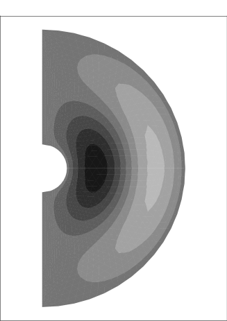
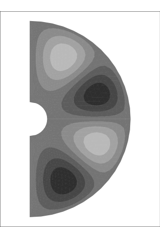
Figure 10: Two independent eigenfunctions in the case of the domain $D$, for $\lambda_{4}=\lambda_{5}\approx 1.9639$.

We are concerned with the cases $n=1$ and $n=4$. For these values, the functions in (36) have, with respect to the azimuthal variable $\theta$, one single bump or 4 consecutive bumps, respectively (see figure 10). As a matter of fact, we have: $\sin\theta P^{\prime}_{1}(\cos\theta)=\sin\theta~{}$ and $~{}\sin\theta P^{\prime}_{4}(\cos\theta)=\frac{5}{2}\sin\theta\cos\theta(7\cos^{2}\theta-3)$. Regarding instead the radial variable $r$, we would like to find suitable linear combinations of the functions in (36), in order to impose homogeneous Dirichlet boundary conditions at $r=1$ and $r=r_{D}$. In agreement with the results obtained by implementing the finite element method, playing with the zeros of Bessel functions, yields:

$$\lambda=\lambda_{4}=\lambda_{5}~{}\approx~{}1.9639~{}~{}~{}~{}~{}~{}~{}~{}{\rm and}~{}~{}~{}~{}~{}~{}~{}~{}~{}~{}r_{D}~{}\approx~{}5.839$$ (37)

These data are now more accurate. The correct assemblage of the radial basis functions can be seen in figure 11. The first picture shows a linear combination of $J_{3/2}$ and $Y_{3/2}$ ($n=1$), the second one a linear combination of $J_{9/2}$ and $Y_{9/2}$ ($n=4$). Up to multiplicative constants, this setting is unique if we impose the boundary conditions at the endpoints of the same interval $[1,r_{D}]$. In a similar way, we can also update the values of table 4 (fourth column), namely: $\lambda_{1}\approx.626$, $\lambda_{2}\approx.980$, $\lambda_{3}\approx 1.432$.

                 

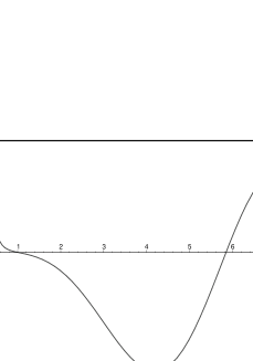
Figure 11: Plots of combinations of Bessel functions of first and second kind, vanishing at $r=1$ and $r=r_{D}$.

Further external shells are obtained by linearly amplifying the domain $D$. In this way, the size of the successive nested shells grows geometrically by a factor $5.839$, and the corresponding frequencies are progressively reduced by the same factor. Like gears of increasing magnitude connected together, the shells transmit their signals far away from the source, through a quantized process, causing a decay of the frequency at each step (see Ref. [1], section 6.1).

As a last example, we examine the case of figure 12, where the curved part of the domain $E$ is an ellipse. We recall that when the Hill’s vortex is perfectly spherical (domain $A$ in figure 6) there is no chance to get coincident eigenvalues (see the first column of table 4). However, by reducing the vertical axis, the situation improves without the help of internal holes. We found out that $\lambda_{4}=\lambda_{5}$ when the ratio between the vertical and the horizontal axis is equal to .6035 (see table 5). The evolution of the solution is expected to be similar to that of figures 8 and 9.

In Ref. [16], predictions and experimental verifications about the formation of stable configurations consisting of an elliptic-shaped Hill’s type vortex, generated by an internal thin vortex ring, are discussed. Further indications might come from our approach, based on the study of $\lambda_{4}$ and $\lambda_{5}$, by simultaneously arranging the eccentricity of the ellipse and the location and the size of the internal vortex. The configuration is going to be similar to the one of figure 4 in Ref. [16]. We tried a few qualitative experiments in this direction, but, having too many degrees of freedom, a careful analysis is a technical exercise that we would prefer to avoid at the moment. Therefore, we do not anticipate any result.

         

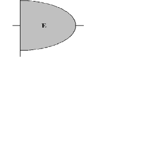
Figure 12: Elliptic section with semi-axis equal to 1 and .6035.

$$\begin{array}[]{|c|c|}\hline\cr&~{}~{}{domain}~{}E{}{}\\ \hline\cr\lambda_{1}&~{}~{}26.96\\ \lambda_{2}&~{}~{}56.97\\ \lambda_{3}&~{}~{}64.53\\ \lambda_{4}&101.95\\ \lambda_{5}&101.99\\ \hline\cr\end{array}$$

Table 5: Eigenvalues corresponding to the domain E of figure 12.

6 Conclusions

With the help of numerical simulations, we demonstrated the possibility of building electromagnetic waves trapped in bounded 3-D regions of space. We did not insist too much on issues related to the performances of the algorithms. We are conscious of the fact that the methods used can be certainly ameliorated, in terms of costs versus accuracy. Nevertheless, this was not our primary concern.

We think that the results we got may have a general validity independently on the field of applications. In fact, the approach we followed, based on the determination of periodic solutions to the wave equation through the analysis of certain eigenvalues of a suitable differential operator, may be applied in several circumstances. For example, as an alternative, this technique may be employed in fluid dynamics (for stable periodic flows), where computations are usually carried out by discretizing the equations by some time-advancing procedure. However, the meaning of the results obtained here is deeper, since they are related to the approximation of a complete system of hyperbolic equations (namely the Maxwell’s equations) and not just to the detection of the flow-field. As a matter of fact, the information carried by our waves is not a scalar density field, but it consists of two separated vector fields: the electric and the magnetic ones. These can be fully expressed by the relations in (28).

A recent subject of research, that could benefit from our investigation, is the detection of quantum vortex rings in superfluid helium (the literature in the field is very rich, see for instance Ref. [17] for a general overview). Note that, in liquid helium, the thickness of these rings is on the order of a few Angstroms. Other related topics might be the study of ball lightning phenomena (see for instance Ref. [18] and Ref. [19]) or ring nebulae and their halos (see for instance Ref. [20]).

Our analysis might inspire interesting applications, that at the moment we are unable to predict. Indeed, we showed that it is possible to detect 3-D regions of space, where an electromagnetic wave, suitably supplied through the boundary, can freely travel without bouncing off the walls. Moreover, we also explained how to build these regions. We are not enough experienced in the field of applications to find an employment for such resonant boxes, but this paper may suggest to some interested reader how to use them to create new tools or improve existing ones.

Finally, we recall that the stability of these structures is a consequence of gravitational modifications of the space-time generated by the movement of the wave itself, according to Einstein’s equation. In fact, the wave travels like a fluid, along closed stream-lines, that turn out to be geodesics of such a modified geometry (see also Ref. [21]). Thus, in the electrodynamic framework, a complete analysis of stability depends on the resolution of a complex relativistic problem. Nevertheless, we hope that the simple investigation carried out in this paper may represent a step ahead towards a better comprehension of the mechanism of vortex formation, whatever the constituents are (fields or real matter).

References

- [1] D. Funaro, Electromagnetism and the Structure of Matter (World Scientific, Singapore, 2008).
- [2] G.K. Batchelor, An Introduction to Fluid Dynamics(Cambridge Univ. Press, 1967).
- [3] T.T. Lim and T.B. Nickels, Vortex rings, Fluid Vortices , ed. S. I. Green (Kluwer Academic, NY, 1995).
- [4] K. Shariff and A. Leonard, Vortex rings,Annual Rev. Fluid Mech. 24, p.235 (1992).
- [5] http://cdm.unimo.it/home/matematica/funaro.daniele/phys.htm
- [6] G.N. Watson, A Treatise on the Theory of Bessel Functions (Cambridge University Press, 1944).
- [7] A. Henrot and M. Pierre, Variation et Optimisation de Formes: Une Analyse Géométrique (Springer-Verlag, Heidelberg, 2005).
- [8] Modulef Installation Page, http://www-rocq.inria.fr/modulef
- [9] P. Laug and P.L. George, Normes d’utilisation et de programmation, Guide MODULEF N. 2 ( INRIA, Paris-Rocquencourt,1992).
- [10] T.J. Maxworthy, The structure and stability of vortex rings, Journal of Fluid Mechanics 51, p.15 (1972).
- [11] D.I. Pullin, Vortex ring formation at tube and orifice openings, Phys. Fluids 22, p.401 (1979).
- [12] S.L. Wakelin and N. Riley, On the formation of vortex rings and pairs of vortex rings, Journal of Fluid Mechanics 332, p.121 (1997).
- [13] P.F. Linden and J.S. Turner, The formation of ‘optimal’ vortex rings, and the efficiency of propulsion devices, Journal of Fluid Mechanics 427, p.61 (2001).
- [14] H.C. Kuo, L.Y. Lin, C.P. Chang and R.T. Williams, The formation of concentric vorticity structures in typhoons, J. Atmos. Sci. 61, p.2722 (2004).
- [15] A. R. Elcrat, B. Fornberg and K.G. Miller, Some steady axissymmetric vortex flows past a sphere, Journal of Fluid Mechanics 433, p.315 (2001).
- [16] I.S. Sullivan, J.J. Niemela, R.E. Hershberger, D. Bolster and R.J. Donnelly, Dynamics of thin vortex rings,Journal of Fluid Mechanics 609, p.319 (2008).
- [17] C.F. Barenghi and R. J. Donnelly, Vortex rings in classical and quantum systems, Fluid Dynamics Research 41, 051401 (2009).
- [18] R. Alanakyan-Yu, Energy capacity of an electromagnetic vortex in the atmosphere, Journal of Experimental and Theoretical Physics 78, p.320 (1994).
- [19] Zou You-Suo, Some physical considerations for unusual atmospheric lights observed in Norway, Physica Scripta 52, p.726 (1995).
- [20] M. Bryce, B. Balick and J. Meaburn, Investigating the Haloes of Planetary Nebulae, Part Four - NGC6720 the Ring Nebula, R.A.S. Monthly Notices 266, p.721 (1994).
- [21] D. Funaro, Electromagnetic radiations as a fluid flow, arXiv: 0911.4848v1.