A covariant investigation of Neutral Vector Mesons:
dynamical properties and electromagnetic decay widths

Abstract

A simple, but fully-covariant model for describing neutral Vector Mesons, in both light and heavy sectors, is briefly illustrated. The main ingredients of our relativistic constituent model are i) an Ansatz for the Bethe-Salpeter vertex for Vector Mesons, and ii) a Mandelstam-like formula for the electromagnetic decay widths. The free parameters of our approach are fixed through a comparison with the valence transverse-momentum distribution, $n(k_{\perp})$, obtained within phenomenological Light-Front Hamiltonian Dynamics models reproducing the mass spectra. Preliminary results for the transverse-momentum distributions, the parton distribution and the electromagnetic decay constants are shown.

1 INTRODUCTION

Aim of this contribution is to illustrate a fully covariant model for describing the electromagnetic (em) decay of neutral Vector Mesons (VM), in both light and heavy sectors (see [1] for a preliminary presentation of our approach). For the present stage, we have considered only the ground states, to be described by using Bethe-Salpeter (BS) amplitudes with a simple analytic form, namely exhibiting only single poles. This assumption allows us to easily perform the analytic integration needed for calculating the constituent quark (CQ) transverse-momentum distribution inside the VMs (see, e.g. Refs. [2] and [3] for the pion case) and then em decay widths. The free parameters present in the Ansatz for each VM are fixed by comparing the so-called valence transverse-momentum distribution, $n(k_{\perp})$, with the same quantity evaluated within a Light-Front Hamiltonian Dynamics (LFHD) approach exploiting the eigenfunctions of two phenomenological mass operators, presented in Refs. [4] and [5], and able to reproduce the VM spectra. It should be pointed out that the free parameters represent an effective way for including some non perturbative features in our analytical Ansatz.

A possible form of the BS amplitude for an interacting $q\bar{q}$ system with $J=1$, can be written as follows

$$\Psi_{\lambda}(k,P)=S(k,m_{1})~{}{\cal V}_{\lambda}(P)~{}S(k-P,m_{2})\times$$

$$\Lambda_{VM}(k,P)$$ (1)

where $S(k,m)=S(k_{on},m)+{\gamma^{+}/(2k^{+})}$ is the Dirac propagator of a constituent quark with mass $m$, $k^{\mu}_{on}\equiv\{k^{-}_{on},k^{+},{\bf k}_{\perp}\}$ with $k^{-}_{on}=(m^{2}+|{\bf k}_{\perp}|^{2})/k^{+}$, $P^{\mu}$ the four-momentum of a VM with mass $P^{2}=M_{VM}^{2}$, $\Lambda_{VM}(k,P)$ the momentum dependence of the BS amplitude, and ${\cal V}_{\lambda}(P)=\epsilon_{\lambda}(P)\cdot V(P)$ with $\epsilon^{\mu}_{\lambda}(P)$ the polarization four-vector ($\lambda$ is the helicity) and $V^{\mu}(k,k-P)$ the Dirac structure given by the following familiar expression, transverse to $P^{\mu}$, (see, e.g., [6])

$$V^{\mu}(P)={M_{VM}\over M_{VM}+m_{1}+m_{2}}~{}\left[\gamma^{\mu}-{P^{\mu}~{}/\!\!\!\!P\over M_{VM}^{2}}+\right.$$

$$\left.+~{}\imath~{}{1\over M_{VM}}~{}\sigma^{\mu\nu}P_{\nu}\right]$$ (2)

Then, the scalar product ${\cal V}_{\lambda}(P)$ reduces to

$${\cal V}_{\lambda}(P)={/\!\!\!\epsilon_{\lambda}\left[M_{VM}-{/\!\!\!\!P}\right]\over M_{VM}+m_{1}+m_{2}}$$ (3)

It should be pointed out that one could have two different $\Lambda_{VM}(k,P)$’s, one for each Dirac structure in ${\cal V}_{\lambda}(P)$ (i.e. $/\!\!\!\epsilon_{\lambda}$ and $/\!\!\!\epsilon_{\lambda}{/\!\!\!\!P}$), but at the present stage we assume a simpler form, with the same $\Lambda_{VM}(k,P)$ for the two structures, that leads to the expected Melosh Rotation factor for a ${}^{3}S_{1}$ system, in the limit of non interacting systems, i.e. $M_{VM}\to M_{free}$ or $P^{\mu}\to P^{\mu}_{free}$ [7]. Therefore the following comparison with the phenomenological LFHD outcomes can be made more strict.

In the preliminary calculations presented in this contribution, the momentum dependence of the BS amplitude is given by the following Ansatz, with only single poles, viz

$$\Lambda_{VM}(k,P)={\cal N}~{}$$

$$\left[k^{2}-m_{1}^{2}+(P-k)^{2}-m_{2}^{2}\right]~{}\Pi_{i=1,3}\times$$

$${1\over\left[k^{2}-m_{R_{i}}^{2}+\imath\epsilon\right]\left[(P-k)^{2}-m_{R_{i}}^{2}+\imath\epsilon\right]}$$ (4)

where $m_{R_{i}}$, $i=1,2,3$ are free parameters (determined as described below), and ${\cal N}$ the normalization factor, that is obtained by imposing the normalization for the BS amplitude in Impulse Approximation, i.e. by adopting constituent quark free propagators. The form chosen for $\Lambda_{VM}(k,P)$ allows one: i) to implement the correct symmetry under the exchange of the quark momenta (for equal mass constituents), as follows from the charge conjugation of the neutral mesons; ii) to regularize the integrals needed in our approach for the evaluation of valence wave functions, decay constants, transverse-momentum distributions, etc.; and iii) to avoid any free propagation in the valence wave function, given the presence of the numerator in $\Lambda_{VM}(k,P)$ (see also [1, 8]).

To determine $m_{R_{i}}$ in Eq. (4), we have introduced the transverse-momentum distribution of a CQ inside the VM, adopting the same definition already applied by de Melo et al. [2] for a covariant description of the pion. In a frame where ${\bf P}_{\perp}={\bf 0}$, one first defines the valence component of the VM state in the standard way (see, e.g., [9]), viz.

$$\Psi^{val}_{VM}(\xi,{\bf k}_{\perp};m_{R_{i}})=\int dk^{-}~{}S(k_{on},m_{1})~{}\times$$

$${\cal V}_{\lambda}(P)~{}\Lambda_{VM}(k,P)S\left((k-P)_{on},m_{2}\right)$$ (5)

with $\xi=k^{+}/P^{+}$. The normalization factor in $\Lambda_{VM}(k,P)$ (cf Eq. (4)) is evaluated in Impulse Approximation by exploiting the total-momentum sum rule, that reads for the plus component as follows

$$P^{+}=~{}{N_{c}\over 2}\int\frac{d^{4}k}{(2\pi)^{4}}~{}{\bar{\Lambda}_{VM}(k,P)\over\left[(k-P)^{2}-m^{2}_{2}+\imath\epsilon\right]}~{}~{}\times$$

$${{\bf T}^{+}_{\lambda,\lambda}(P,k)\over\left[(k-P)^{2}-m^{2}_{2}+\imath\epsilon\right]}{\Lambda_{VM}(k,P)\over(k^{2}-m^{2}_{1}+\imath\epsilon)}$$ (6)

with $N_{c}=3$ and

$${\bf T}^{+}_{\lambda,\lambda}(P,k)=Tr\left\{{\cal V}_{\lambda}(P)~{}\times\right.$$

$$\left.({/\!\!\!k}-/\!\!\!{P}+m_{2})\gamma^{+}~{}(/\!\!\!{k}-/\!\!\!{P}+m_{2})~{}\times\right.$$

$$\left.{\cal V}^{\dagger}_{\lambda}(P)~{}(/\!\!\!{k}+m_{1})\right\}=$$

$$=-2(P^{+}-k^{+})\left[\phantom{{(k^{-}-k^{-}_{on})\over 2}}{\cal T}^{+}(P,k,on)+\right.$$

$$\left.{(k^{-}-k^{-}_{on})\over 2}{\cal T}^{+}(P,k,ist)\right]$$ (7)

In Eq. (7), ${\cal T}^{+}(P,k,on)$ and ${\cal T}^{+}(P,k,ist)$ are the on-shell and the instantaneous contributions, respectively, according to the well-known decomposition of the Dirac propagator (see below Eq. (1)). Their explicit expressions will be given elsewhere [10]. Notice that, after performing the trace, the dependence upon the helicity disappears, and therefore its presence in ${\bf T}^{+}_{\lambda,\lambda}(P,k)$ becomes dummy.

Table 1: The mass eigenvalues for the ground states of the neutral VMs investigated in this contribution compared with the corresponding experimental values. The mass operator corresponds to the one in Ref. [4] (see [10] for details). The quark masses adopted for the actual evaluation are also listed.

VM	$m_{q}(MeV)$	$M^{th}_{VM}$ (MeV)	$M^{exp}_{VM}$ (MeV)
$\rho$	328	777.0	775.500 $\pm$ 0.4
$\phi$	449	1020.7	1019.455 $\pm$ 0.020
$J/\psi$	1559	3082.9	3096.916 $\pm$ 0.011
$\Upsilon$	4891	9537.2	9460.300 $\pm$ 0.268

Table 2: The same as in Table 1, but for the mass operator of Ref. [5].

VM	$m_{q}(MeV)$	$M^{th}_{VM}$ (MeV)	$M^{exp}_{VM}$ (MeV)
$\rho$	220	777	775.500 $\pm$ 0.4
$\phi$	419	1016	1019.455 $\pm$ 0.020
$J/\psi$	1628	3091	3096.916 $\pm$ 0.011
$\Upsilon$	4977	9460	9460.300 $\pm$ 0.268

Finally, let us introduce the valence transverse-momentum distribution, $n_{val}(k_{\perp})$, given by

$$n_{val}(k_{\perp})={N_{c}\over(2\pi)^{3}\left[P^{+}\right]^{2}P^{VM}_{q\bar{q}}}\int_{0}^{2\pi}d\theta_{k_{\perp}}~{}\times$$

$$\int_{0}^{1}d\xi{{\cal T}^{+}(P,k,on)\over\xi~{}(1-\xi)}~{}|\Phi^{val}_{VM}(\xi,{\bf k_{\perp}};m_{R_{i}})|^{2}$$ (8)

where $P^{VM}_{q\bar{q}}$ is the probability of the valence component, given by

$$P^{VM}_{q\bar{q}}={N_{c}\over(2\pi)^{3}\left[P^{+}\right]^{2}}\int_{0}^{1}{d\xi\over\xi~{}(1-\xi)}~{}\times$$

$$\int d{\bf k}_{\perp}~{}{\cal T}^{+}(P,k,on)~{}|\Phi^{val}_{VM}(\xi,{\bf k_{\perp}};m_{R_{i}})|^{2}$$ (9)

and

$$\Phi^{val}_{VM}(\xi,{\bf k_{\perp}};m_{R_{i}})=~{}k^{+}~{}(P-k)^{+}~{}\int dk^{-}~{}\times$$

$${\Lambda_{VM}(k,P)\over(k^{2}-m^{2}_{1})~{}\left[(k-P)^{2}-m^{2}_{2}\right]}$$ (10)

In a LFHD approach (see, e.g. [2] and references quoted therein), one has

$$n^{HD}_{VM}(k_{\perp})=\int_{0}^{2\pi}d\theta_{k_{\perp}}\int_{0}^{1}{d\xi~{}M^{2}_{free}\over\xi(1-\xi)}~{}\times$$

$$|\psi_{VM}(\xi,{\bf k}_{\perp})|^{2}$$ (11)

where $\psi_{VM}(\xi,{\bf k}_{\perp})$ is the eigenfunction of a relativistic mass operator and $M^{2}_{free}=(m^{2}+|{\bf k}_{\perp}|^{2})/\xi(1-\xi)$. In order to implement our procedure for fixing the free parameters in $\Lambda_{VM}$, we have first evaluated $n^{HD}_{VM}(k_{\perp})$ by adopting the eigenfunctions obtained by using the model mass operators of both Refs. [4] and [5], and then we have minimized the difference $|n_{val}(k_{\perp})-n^{HD}_{VM}(k_{\perp})|$. It should be pointed out that the VM spectra are satisfactorily reproduced for each VM investigated in this contribution. As an example of the reliability of the adopted LFHD models, the masses of the considered neutral VMs for the ground states are compared with the corresponding experimental values in Tables 1 and 2 for the mass operators of Refs. [4] and [5], respectively. Indeed, also the masses of the first three/four (depending upon the considered VM) excited states are well reproduced by the model mass operators.

Once the parameters have been determined, one can calculate both static (e.g., em decay rates) and dynamical (e.g. parton distributions) quantities. For completing this section, devoted to the general presentation of the formalism, we give the expression of the parton distribution, i.e.

$$q(\xi)=\int dk_{\perp}~{}k_{\perp}~{}f_{1}(\xi,k_{\perp})$$ (12)

in terms of the chiral-even transverse-momentum distribution, $f_{1}(\xi,k_{\perp})$, (see, e.g. [10] and [3] for the pion case), that yields the distribution of a constituent inside the meson with the longitudinal and transverse components of the LF-momentum. It reads

$$f_{1}(\xi,k_{\perp})=~{}{N_{c}\over 4P^{+}}~{}\int^{2\pi}_{0}d\theta_{k_{\perp}}~{}\int\frac{dk^{-}}{(2\pi)^{4}}~{}\times$$

$$~{}{\bar{\Lambda}_{VM}(k,P)\over\left[(k-P)^{2}-m^{2}_{2}+\imath\epsilon\right]}{{\bf T}^{+}_{\lambda,\lambda}(P,k)\over\left[(k-P)^{2}-m^{2}_{2}+\imath\epsilon\right]}\times$$

$${\Lambda_{VM}(k,P)\over(k^{2}-m^{2}_{1}+\imath\epsilon)}$$ (13)

The explicit expression of $f_{1}(\xi,k_{\perp})$ will be presented elsewhere [10].

2 THE MANDELSTAM FORMULA FOR THE EM DECAY CONSTANT

In order to evaluate the em decay constant, $f_{VM}$, we adopt a Mandelstam-like formula [11] (see also [12] and [3] for the pion case). The starting point is the macroscopic definition of $f_{VM}$, through the transition matrix element of the em current for a given neutral VM, viz

$$\langle 0|J^{\mu}(0)|P,\lambda\rangle=\imath\sqrt{2}f_{VM}\epsilon_{\lambda}^{\mu}$$ (14)

Let us remind that the decay constant $f_{VM}$ is related to the em decay width as follows

$$\Gamma^{VM}_{e^{+}e^{-}}=\frac{8\pi\alpha^{2}}{3}\frac{|f_{VM}|^{2}}{M_{VM}^{3}}$$ (15)

In our model, the transition matrix element in Eq. (14) can be approximated microscopically à la Mandelstam through

$$\langle 0|J^{\mu}(0)|P,\lambda\rangle={\cal Q}_{VM}~{}{{N_{c}}{\cal N}\over(2\pi)^{4}}\int d^{4}k~{}\times$$

$${\Lambda_{VM}(k,P,m_{1},m_{2})\over(k^{2}-m^{2}_{1}+\imath\epsilon)~{}[(P-k)^{2}-m^{2}_{2}+\imath\epsilon]}\times$$

$${\rm Tr}[{\cal V}_{\lambda}(P)~{}(/\!\!\!k-/\!\!\!P+m_{2})\gamma^{\mu}(/\!\!\!k+m_{1})]$$ (16)

where

$${\cal Q}_{\rho}={(Q_{u}-Q_{d})\over\sqrt{2}}\quad\quad{\cal Q}_{\phi}=Q_{s}$$

$${\cal Q}_{J/\Psi}=Q_{c}\quad\quad{\cal Q}_{\Upsilon}=Q_{b}$$

with $Q_{i}$ the quark charge. The lengthy algebra for evaluating the analytic integrations in Eq. (16) will be reported elsewhere [10].

3 PRELIMINARY RESULTS

In Figs. 1 and 2, the valence transverse-momentum distributions (cf Eq. (8)) for $\rho$, $\phi$, $J/\psi$ and $\Upsilon$ are shown, for different sets of the free parameters. In order to get some dynamical input, in Fig. 1 the free parameters of our Ansatz (see Eq. (1)) have been determined through the model of Ref. [4], while in Fig. 2 through the model of Ref. [5]. In the figures the distributions are multiplied by a factor $k_{\perp}$, to have an immediate intuition of the transverse-momentum region relevant in the evaluation of the valence probabilities. It is worth noting that the long tail of the heavy VM is an expected feature. In Figs. 3 and 4, the parton distributions are presented. As it is shown, the general behavior at the end-points and the accumulation of the distribution for $x=1/2$ as the CQ mass increases are recovered by using our Ansatz.

Finally, in Tables 3 and 4, the preliminary values for the em decay widths, for the two different choices of the free parameters, are compared with the corresponding experimental data. It should be pointed out that while the model of Ref. [4] yields reasonable results for the light sector (let us remind that the confining interaction for the squared mass operator of [4] is parabolic), in the heavy sector the model of Ref. [5] seems to behave better (for this model a linear confining interaction is considered in the mass operator). Such a comparison suggests that an improved description of the confining interaction for the squared mass operator of Ref. [4] could lead the theoretical predictions of the em decays closer to the experimental ones.

Table 3: Preliminary VM em decay widths, calculated using our Ansatz, (1), and the free parameters determined through the comparison with the eigenfunctions of the model [4] for the mass operator.

VM	$\Gamma_{e^{+}e^{-}}^{th}$ (keV)	$\Gamma_{e^{+}e^{-}}^{exp}$ (keV) [13]
$\rho$	8.579	7.04 $\pm$ 0.06
$\phi$	1.952	1.27 $\pm$ 0.04
$J/\psi$	2.526	5.55 $\pm$ 0.14
$\Upsilon$	0.187	1.340$\pm$ 0.018

Table 4: The same as in table 1, but using the eigenfunctions of the model [5] to fix the free parameters.

VM	$\Gamma_{e^{+}e^{-}}^{th}$ (keV)	$\Gamma_{e^{+}e^{-}}^{exp}$ (keV) [13]
$\rho$	24.791	7.04 $\pm$ 0.06
$\phi$	4.342	1.27 $\pm$ 0.04
$J/\psi$	7.102	5.55 $\pm$ 0.14
$\Upsilon$	0.493	1.340$\pm$ 0.018

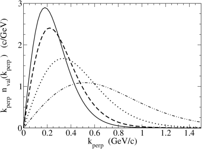
Figure 1: Valence transverse-momentum distributions for a constituent inside $\rho$, $\phi$, $J/\Psi$ and $\Upsilon$ vs the quark transverse momentum. The normalization is $\int k_{\perp}~{}d{k}_{\perp}~{}n_{val}(k_{\perp})=1$. Solid line: $\rho$; dashed line: $\phi$; dotted line: $J/\Psi$; double-dot-dashed line: $\Upsilon$. The free parameters in (1), have been determined through the comparison with the eigenfunctions of the model [4].

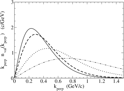
Figure 2: The same as in Fig. 1, but using the eigenfunctions of the model [5] to fix the free parameters in (1).

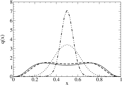
Figure 3: Valence distributions for a constituent inside $\rho$, $\phi$, $J/\Psi$ and $\Upsilon$ vs $x$, with normalization $\int d\xi~{}q(\xi)=1$. The same line convention as in Fig. 1 is adopted. The free parameters in (1), have been determined through the comparison with the eigenfunctions of the model [4].

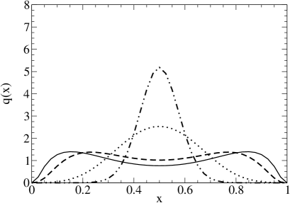
Figure 4: The same as in Fig. 3, but using the eigenfunctions of the model [5] to fix the free parameters in (1).

4 CONCLUSIONS

The preliminary results for some static and dynamical quantities for neutral VM, obtained within our covariant description, both in the light and the heavy sectors, have been shortly presented. After calculating the valence wave functions, Eq. (5), and the transverse-momentum distributions, Eq. (8), we have fixed the three parameters in our Ansatz for the Bethe-Salpeter amplitude through a comparison with the transverse-momentum distribution obtained within a Light-Front Hamiltonian Dynamics approach. The eigenvectors of two different mass operators, corresponding to Ref. [4] and Ref. [5], have been considered in order to perform the comparison. Then, we have evaluated the parton distributions and the em decay constants (cf Table 3 and Table 4).

The work in progress will substantially improve the present calculations, in two respect: both introducing a more refined Ansatz for the BS amplitude and considering new phenomenological mass operators.

This work was partially supported by the Brazilian agencies CNPq and FAPESP and by Ministero della Ricerca Scientifica e Tecnologica. S.P. acknowledges the ”Fondazione Della Riccia” for supporting her research activity and the hospitality of ITA.

References

• [1] T. Frederico, E. Pace, S. Pisano and G. Salmè, arXiv:0802.3144.
• [2] J. P. B. C. de Melo, T. Frederico, E. Pace and G. Salmè, Nucl. Phys. A 707, 399 (2002).
• [3] T. Frederico, E. Pace, B. Pasquini and G. Salmè, Phys. Rev. D 80, 054021 (2009).
• [4] L. A. M. Salcedo, J. P. B. C. de Melo, D. Hadjimichel and T. Frederico, Eur. Phys. Jour. 27 213 (2006).
• [5] S. Godfrey and N. Isgur, Phys. Rev. D 32, 189 (1985).
• [6] Chueng-Ryong Ji, P.L. Chung and Stephen Cotanch, Phys. Rev. D 45, 4214 (1992).
• [7] W. Jaus, Phys. Rev. D 44, 2851 (1991).
• [8] F. Gross, M.T. Peña and G. Ramalho, Phys. Rev. C 77, 015202 (2008).
• [9] Dae Sung Hwang and V. A. Karmanov, Nucl. Phys. B 696, 413 (2004).
• [10] T. Frederico, E. Pace, S. Pisano and G. Salmè to be published.
• [11] S. Mandelstam, Proc. Royal Soc. (London) A233, 248 (1956).
• [12] J. P. B. C. de Melo, T. Frederico, E. Pace and G. Salmè, Phys. Rev. D 73, 074013 (2006).
• [13] C. Amsler et al. (Particle Data Group), Phys. Lett. B 667, 1 (2008).