Phantom boundary crossing and anomalous growth index of fluctuations in viable $f(R)$ models of cosmic acceleration

Abstract

Evolution of a background space-time metric and sub-horizon matter density perturbations in the Universe is numerically analyzed in viable $f(R)$ models of present dark energy and cosmic acceleration. It is found that viable models generically exhibit recent crossing of the phantom boundary $w_{\rm DE}=-1$. Furthermore, it is shown that, as a consequence of the anomalous growth of density perturbations during the end of the matter-dominated stage, their growth index evolves non-monotonically with time and may even become negative temporarily.

RESCEU-5/10

I Introduction

The physical origin of the dark energy (DE) which is responsible for an accelerated expansion of the current Universe is one of the largest mysteries not only in cosmology but also in fundamental physics review . Although the standard spatially flat ${\rm\Lambda}$-Cold-Dark-Matter (${\rm\Lambda CDM}$) model is consistent with all kinds of current observational data WMAP7 , some tentative deviations from it have been reported recently Shafieloo:2009ti ; Bean:2009wj which, if proven to be not due to systematic and other errors, may eventually rule out an exact cosmological constant. Furthermore, in the ${\rm\Lambda CDM}$ model, the cosmological term is regarded as a new fundamental constant whose observed value is much smaller than any other energy scale known in physics. So, its understanding in fundamental physics is lacking today, although some non-perturbative effects may generate such a small quantity Yokoyama:2001ez . On the other hand, we know that “primordial DE,” which is responsible for inflation in the early universe S80 ; sato ; guth , is not identical to the cosmological constant, in particular, it is not stable and eternal. Hence it is natural to seek for non-stationary models of the current DE, too.

Among them, $f(R)$ gravity which modifies and generalizes the Einstein gravity by incorporating a new phenomenological function of the Ricci scalar $R$, $f(R)$, provides a self-consistent and non-trivial alternative to ${\rm\Lambda CDM}$ model, see e.g. Ref. SF08 for a recent review. This theory is a special class of the scalar-tensor theory of gravity with the vanishing Brans-Dicke parameter $\omega_{BD}$ Chiba:2003ir ; Tsujikawa:2008uc . It contains a new scalar degree of freedom dubbed ”scalaron” in Ref. S80 , thus, it is a non-perturbative generalization of the Einstein gravity.

This additional degree of freedom imposes a number of conditions on viable functional forms of $f(R)$. In particular, in order to have the correct Newtonian limit for $R\gg R_{0}\equiv R(t_{0})\sim H_{0}^{2}$ where $t_{0}$ is the present moment and $H_{0}$ is the Hubble constant, as well as the standard matter-dominated stage with the scale factor behaviour $a(t)\propto t^{2/3}$ driven by cold dark matter and baryons, the following conditions should be fulfilled:

$$|f(R)-R|\ll R,~{}~{}|f^{\prime}(R)-1|\ll 1,~{}~{}Rf^{\prime\prime}(R)\ll 1,~{}~{}R\gg R_{0}~{},$$ (1)

where the prime denotes the derivative with respect to the argument $R$. In addition, the stability condition $f^{\prime\prime}(R)>0$ has to be satisfied that guarantees that the standard matter-dominated Friedmann stage remains an attractor with respect to an open set of neighboring isotropic cosmological solutions in $f(R)$ gravity. In quantum language, this condition means that scalaron is not a tachyon. Note that the other stability condition, $f^{\prime}(R)>0$, which means that gravity is attractive and graviton is not a ghost, is automatically fulfilled in this regime. Specific functional forms that satisfy all these conditions have been proposed in Refs. Hu:2007nk ; AB07 ; Starobinsky:2007hu etc., and much work has been done on their cosmological consequences.

In the previous paper Motohashi:2009qn we calculated evolution of matter density fluctuations in viable $f(R)$ models Hu:2007nk ; Starobinsky:2007hu in the limiting case $R\gg R_{0}$ during the matter-dominated stage and found an analytic expression for them. In this paper we extend the previous analysis and perform numerical calculations of the evolution of both background space-time and density fluctuations for the particular $f(R)$ model of Ref. Starobinsky:2007hu without such restriction on $R$. As a result, we have found the phantom boundary crossing at an intermediate redshift $z\lesssim 1$ for the background space-time metric and an anomalous behaviour of the growth index of fluctuations.

The rest of the paper is organized as follows. In §2 we introduce evolution equations for the homogeneous and isotropic background and present results of numerical integration. In §3 we report numerical solutions for the evolution of density fluctuations and other observables. Section 4 is devoted to conclusions and discussion.

II Evolution of the background Universe

We adopt the following action with a four-parameter family of $f(R)$ models:

$$S =\frac{1}{16\pi G}\int d^{4}x\sqrt{-g}f(R)+S_{m},$$ (2)

$$f(R) =R+\lambda R_{s}\left[\left(1+\frac{R^{2}}{R_{s}^{2}}\right)^{-n}-1\right]+\frac{R^{2}}{6M^{2}},$$ (3)

where $n,~{}\lambda,~{}R_{s}$, and $M$ are model parameters and $S_{m}$ is the action of the matter content which is assumed to be minimally coupled to gravity (thus, the action (2) is written in the Jordan frame). This is the model of Ref. Starobinsky:2007hu modified by the last term in (3) borrowed from the inflationary model of Ref. S80 . This term is introduced for several purposes associated with high-curvature behaviour of the theory. One of them, as explained in Ref. Starobinsky:2007hu , is to avoid excessive growth of the scalaron mass, $m_{s}^{2}=1/3f^{\prime\prime}(R)$ in the regime (1), towards the early Universe, $t\to 0$. The other one is to remove the additional and undesirable “Big Boost” singularity which can arise in the original models Hu:2007nk ; AB07 ; Starobinsky:2007hu as was shown in Ref. F08 (see Refs. Motohashi:2009qn ; TSC09 ; ABS09 for more discussion on this point). The value of $M$ should be sufficiently large in order not to destroy the standard cosmology of the present and early Universe. In particular, the values of $M$ considered in Refs. D08 ; KM09 are not high enough for this purpose, because $M$ should not be smaller than the Hubble parameter $H(t)$ during the $N\sim 60$ last e-folds of inflation in the early Universe in order to avoid overproduction of relic scalarons, as well as to solve other cosmological problems. In fact, if we take $M\approx 3\times 10^{13}$ GeV, the scalaron itself can act as an inflaton S80 and generate primordial scalar (adiabatic) and tensor perturbations MC81 ; S83 with the amplitudes and slopes of their power spectra in agreement with all observational data available today. Note, however, that as shown in Ref. ABS09 , such a ”unified” model describing both primordial DE driving inflation in the early Universe and present DE driving recent acceleration of the Universe in the scope of $f(R)$ gravity leads to slightly different predictions for parameters of the primordial perturbation spectra, as compared to the purely inflationary model with $\lambda R_{s}=0$, due to a change in the number of observable e-folds of inflation $N$ caused by different evolution of the Universe during generation and heating of usual matter after inflation. Furthermore, in this unified model the term in the square brackets in (3) should be modified for $|R|<R_{0}$ in such a way as to ensure the fulfillment of the stability condition $f^{\prime\prime}(R)>0$ in this region, too.

So, we take this value of $M$ and assume that the evolution of the Universe is identical to that in the standard ${\rm\Lambda CDM}$ model at high redshifts without any relic scalaron oscillations. Then the $R^{2}/6M^{2}$ term is totally negligible in the epoch we are concerned here. Therefore, we do not include its contribution below.

We can express field equations derived from the action in the following Einsteinian form.

$$R^{\mu}_{\nu}-\frac{1}{2}\delta^{\mu}_{\nu}R=-8\pi G\left(T^{\mu}_{\nu(m)}+T^{\mu}_{\nu({\rm DE})}\right),$$ (4)

where

$$8\pi GT^{\mu}_{\nu({\rm DE})}\equiv{\cal{F}}^{\prime}(R)R^{\mu}_{\nu}-\frac{1}{2}{\cal{F}}(R)\delta^{\mu}_{\nu}+(\nabla^{\mu}\nabla_{\nu}-\delta^{\mu}_{\nu}\square){\cal{F}}^{\prime}(R),~{}~{}~{}{\cal{F}}(R)\equiv f(R)-R$$ (5)

(the sign conventions here are the same as in Ref. Starobinsky:2007hu ). Working in the spatially flat Friedmann-Robertson-Walker (FRW) space-time with the scale factor $a(t)$, we find

$$3H^{2} =8\pi G\rho-3{\cal{F}}^{\prime}H^{2}+\frac{1}{2}({\cal{F}}^{\prime}R-{\cal{F}})-3H\dot{{\cal{F}}}^{\prime},$$ (6)

$$2\dot{H} =-8\pi G\rho-2{\cal{F}}^{\prime}\dot{H}-\ddot{{\cal{F}}}^{\prime}+H\dot{{\cal{F}}}^{\prime},$$ (7)

where $H$ is the Hubble parameter and $\rho$ is the energy density of the material content which we assume to consist of non-relativistic matter.

From (5) the effective energy density and pressure of dark energy can be expressed as

$$8\pi G\rho_{\rm DE}=\frac{1}{2}({\cal{F}}^{\prime}R-{\cal{F}})-3H^{2}{\cal{F}}^{\prime}-3H\dot{{\cal{F}}}^{\prime}=-3H\dot{R}{\cal{F}}^{\prime\prime}+3(H^{2}+\dot{H}){\cal{F}}^{\prime}-\frac{1}{2}{\cal{F}},$$ (8)

$$8\pi G(\rho_{\rm DE}+P_{\rm DE})=2\dot{H}{\cal{F}}^{\prime}-H\dot{{\cal{F}}}^{\prime}+\ddot{{\cal{F}}}^{\prime},$$ (9)

respectively, where $R=12H^{2}+6\dot{H}$. We define the DE equation of state parameter $w_{\rm DE}$ by the ratio $w_{\rm DE}\equiv P_{\rm DE}/\rho_{\rm DE}$.

With the appropriate initial condition after cosmic inflation mentioned above, ${\cal{F}}$ takes an asymptotically constant value ${\cal{F}}=-\lambda R_{s}$ at high redshift (apart from the $R^{2}/6M^{2}$ term which we neglect here). In this regime, evolution of the Universe is the same as that obtained from the Einstein action with a cosmological constant $\Lambda(\infty)=\lambda R_{s}/2$. The scale factor therefore evolves as

$$a=a_{i}\left(\frac{16\pi G\rho_{i}}{\lambda R_{s}}\right)^{\frac{1}{3}}\sinh^{\frac{2}{3}}\left(\sqrt{\frac{3\lambda R_{s}}{8}}t\right)\cong a_{i}\left(\frac{t}{t_{i}}\right)^{\frac{2}{3}},$$ (10)

where the suffix $i$ denotes quantities at an initial time $t=t_{i}$.

The time dependence of $\rho_{\rm DE}$ is mainly governed by the first term in the right-most expression of (8) initially. Since $\dot{R}<0$ and ${\cal{F}}^{\prime\prime}>0$ for stability, this means that the effective energy density of dark energy increases with time in this regime. Therefore, DE exhibits the phantom behaviour, $w_{\rm DE}<-1$, during the matter-dominated stage with $z>1$, which lasts only temporarily because the late-time asymptotic de Sitter stage has an effective cosmological constant smaller than $\Lambda(\infty)$. So, $\rho_{\rm DE}$ stops growing after the end of the matter-dominated stage and begins to decrease.

Indeed, as shown in Ref. Starobinsky:2007hu , the late-time asymptotic de Sitter solution has a curvature $R\equiv R_{1}\equiv x_{1}R_{s}$ where $x_{1}$ is the maximal solution of the equation,

$$\lambda=\frac{x(1+x^{2})^{n+1}}{2\left[(1+x^{2})^{n+1}-1-(n+1)x^{2}\right]}.$$ (11)

It satisfies the inequality $x_{1}<2\lambda$, so that $\Lambda(R_{1})=R_{1}/4<\Lambda(\infty)$. These inequalities are saturated in the limit $n\gg 1$ for fixed $x_{1}$, or $x_{1}\gg 1$ for fixed $n$. In these cases cosmic evolution is indistinguishable from the standard ${\rm\Lambda CDM}$ model.

Thus, this model naturally realizes crossing of the phantom boundary $w_{\rm DE}=-1$ in a recent epoch. Note that phantom behaviour of DE is generic in its models based on the scalar-tensor gravity BEPS00 which includes the $f(R)$ theory. Here we see that it is realized in all simplest stable $f(R)$ models of present DE.

The stability condition of this future de Sitter solutionMSS88 , $f^{\prime}(R_{1})>R_{1}f^{\prime\prime}(R_{1})$, imposes the following constraint on $x_{1}$.

$$(1+x_{1}^{2})^{n+2}>1+(n+2)x_{1}^{2}+(n+1)(2n+1)x_{1}^{4},$$ (12)

which is stronger than any other constraint discussed above. For each $n$ we can find $x_{1}$ which marginally satisfies (12) and gives the minimal allowed value of $\lambda$. Numerically we find $(n,x_{1\min},\lambda_{\min})=(2,1.267,0.9440),(3,1.041,0.7259)$, and $(4,0.9032,0.6081)$ for each $n$, respectively (if $n=2$, the analytic expression for $x_{1\min}$ is $x_{1\min}^{2}=\sqrt{13}-2$). For comparison, the analytic results for $n=1$ are $x_{1\min}=\sqrt{3}\approx 1.732,~{}\lambda_{\min}=8/(3\sqrt{3})\approx 1.540$.

We numerically solve evolution equation (7) using (6) to check numerical accuracy, taking $t_{i}$ at the epoch when matter density parameter took $\Omega_{i}=16\pi G\rho_{i}/(16\pi G\rho_{i}+\lambda R_{s})=0.998$. We determine the current epoch by the requirement that the value of $\Omega$ takes the observed central value $\Omega_{0}=0.27$ and $R_{s}$ is fixed so that the current Hubble parameter $H_{0}=72$km/s/Mpc is reproduced. We find the ratio $R_{s}/H_{0}^{2}$ is well fit by a simple power-law $R_{s}/H_{0}^{2}=c_{n}\lambda^{-p_{n}}$ with $(n,c_{n},p_{n})=(2,4.16,0.953),~{}(3,4.12,0.837),$ and $(4,4.74,0.702)$, respectively, whereas in the ${\rm\Lambda CDM}$ limit it would behave as $R_{s}/H_{0}^{2}=6(1-\Omega_{0})/\lambda\simeq 4.38\lambda^{-1}$.

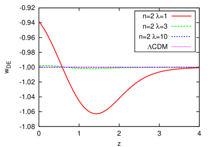
(a) Evolution of $w_{\rm DE}$ for different values of $\lambda$ with $n=2$.

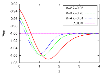
(b) Evolution of $w_{\rm DE}$ for $\lambda_{\min}$ for $n=2,3,$ and 4.

Figure 1: Evolution of the equation-of-state parameter of effective dark energy.

Figures 1 depict evolution of $w_{\rm DE}$ as a function of redshift $z$ where phantom crossing is manifest. As expected, it approaches $w_{\rm DE}=-1=\text{constant}$ as we increase $\lambda$ for fixed $n$. For minimal allowed values of $\lambda$, deviations from $w_{\rm DE}=-1$ are observed at $\sim 5\%$ level in both directions for $z\lesssim 2$ independently of $n$. Such behaviour of $w_{\rm DE}$ is well admitted by all most recent observational data, see e.g. Ref. WMAP7 . The average value of $w_{\rm DE}$ over the interval $0\leq z\leq 1$ to which all BAO and most of SN data refer is very close to $-1$. Moreover, in this range (but not for larger values of $z$), the behaviour of $w_{\rm DE}$ for minimal allowed values of $\lambda$ (i.e. for largest possible deviations from the ${\rm\Lambda CDM}$ background model) is well fitted by the CPL fitCPL $w_{\rm DE}(z)=w_{0}+w_{a}z/(1+z)$ with $(n,\lambda_{\rm min},w_{0},w_{a})=$ $(2,0.95,-0.92,-0.23)$, $(3,0.73,-0.94,-0.22)$ and $(4,0.61,-0.96,-0.21)$, respectively. $|1+w_{0}|$ and $|w_{a}|$ decrease slowly for larger values of $n$. These values of $w_{0}$ and $w_{a}$ lie very close to the center of the $68\%$ and $95\%$ CL ellipses for all combined data in Fig. 13 of Ref. WMAP7 .

As explained above, this phantom crossing behaviour is not peculiar to the specific choice of the function (3) but a generic one in models which satisfy the stability condition ${\cal{F}}^{\prime\prime}>0$. Indeed, a similar behaviour has been observed in other $f(R)$ DE models, too Martinelli:2009ek ; ABS09 . We also note that different definitions of $\rho_{\rm DE}$, $P_{\rm DE}$, and $w_{\rm DE}$ have been used in literature Amendola:2007nt which lead to different behaviour of $w_{\rm DE}$.

Although the behaviour of dark energy is quite different depending on model parameters, the total expansion factor $a_{0}/a_{i}$ from the epoch $\Omega_{i}=0.998$ to the present varies only between $a_{0}/a_{i}=10.8$ and 11, the latter corresponding to the value in the ${\rm\Lambda CDM}$ model.

We have also calculated the quantity $B(z)=(f^{\prime\prime}/f^{\prime})(dR/d\ln H)$ introduced in Ref. Song:2006ej at present time. We have found $B(0)=0.21$, $6.1\times 10^{-5}$, and $0.17$, for $(n,\lambda)=(2,0.95)$, $(2,8)$, and $(4,0.61)$, respectively.

III Density fluctuations

We now turn to evolution of density fluctuations. In $f(R)$ gravity, the evolution equation of density fluctuations, $\delta$, deeply in the sub-horizon regime is given by Zhang:2005vt ; Tsujikawa:2007gd

$$\ddot{\delta}+2H\dot{\delta}-4\pi G_{\text{eff}}\rho\delta=0,$$ (13)

where

$$G_{\text{eff}}=\frac{G}{F}\frac{1+4\frac{k^{2}}{a^{2}}\frac{F^{\prime}}{F}}{1+3\frac{k^{2}}{a^{2}}\frac{F^{\prime}}{F}},~{}~{}~{}F(R)\equiv f^{\prime}(R).$$ (14)

This equation reduces to the correct evolution equation for all wavenumbers for the CDM model in the Einstein gravity where $F=1$.

In the previous paperMotohashi:2009qn we obtained an analytic solution in the high-curvature regime when the scale factor evolves as $a(t)\propto t^{2/3}$ and $F$ takes the asymptotic form

$$F\simeq 1-2n\lambda\left(\frac{R}{R_{s}}\right)^{-2n-1}\equiv 1-\left(\frac{R}{R_{c}}\right)^{-N-1},$$ (15)

with the following correspondence:

$$N=2n~{}~{}~{}{\rm and}~{}~{}~{}R_{c}=R_{s}(2n\lambda)^{1/(2n+1)}.$$ (16)

The two independent solutions of (13) in this regime read

$$\delta_{\mbox{\boldmath\tiny${k}$}}(t)=\delta_{i\mbox{\boldmath\tiny${k}$}}\left(\frac{t}{t_{i}}\right)^{\frac{-1\pm 5}{6}}$$

$$\times\,_{2}F_{1}\left(\frac{\pm 5-\sqrt{33}}{4(3N+4)},\frac{\pm 5+\sqrt{33}}{4(3N+4)};1\pm\frac{5}{2(3N+4)};-3\frac{(N+1)k^{2}}{a_{i}^{2}R_{c}^{2}}\left(\frac{t}{t_{i}}\right)^{2N+8/3}\right)$$ (17)

in terms of the hypergeometric functionMotohashi:2009qn . In the following discussion, we consider the upper sign solution only, because the other solution corresponds to the decaying mode and is singular at $t\to 0$. Then the solution behaves as

$$\delta_{\mbox{\boldmath\tiny${k}$}}(t)\xrightarrow[]{t\to 0}\delta_{i\mbox{\boldmath\tiny${k}$}}\left(\frac{t}{t_{i}}\right)^{\frac{2}{3}}~{}~{}{\rm and}~{}~{}\delta_{\mbox{\boldmath\tiny${k}$}}(t)\xrightarrow[]{t\to\infty}\delta_{i\mbox{\boldmath\tiny${k}$}}C(k)\left(\frac{t}{t_{i}}\right)^{\frac{-1+\sqrt{33}}{6}},$$ (18)

respectively. The transfer function, $C(k)$, is given by

$$C(k) =\frac{\Gamma\left(1+\frac{5}{2(3N+4)}\right)\Gamma\left(\frac{\sqrt{33}}{2(3N+4)}\right)}{\Gamma\left(1+\frac{5+\sqrt{33}}{4(3N+4)}\right)\Gamma\left(\frac{5+\sqrt{33}}{4(3N+4)}\right)}\left[\frac{3(N+1)k^{2}}{a_{i}^{2}R_{c}}\left(\frac{3R_{c}t_{i}^{2}}{4}\right)^{N+2}\right]^{\frac{-5+\sqrt{33}}{4(3N+4)}}$$

$$=\frac{\Gamma\left(1+\frac{5}{4(3n+2)}\right)\Gamma\left(\frac{\sqrt{33}}{4(3n+2)}\right)}{\Gamma\left(1+\frac{5+\sqrt{33}}{8(3n+2)}\right)\Gamma\left(\frac{5+\sqrt{33}}{8(3n+2)}\right)}\left[\frac{6n\lambda(2n+1)k^{2}}{a_{i}^{2}R_{s}}\left(\frac{3R_{s}t_{i}^{2}}{4}\right)^{2(n+1)}\right]^{\frac{-5+\sqrt{33}}{8(3n+2)}},$$ (19)

where

$$t_{i}=\frac{2}{3}\sqrt{\frac{6}{\lambda R_{s}}}\sinh^{-1}\sqrt{\frac{1-\Omega_{i}}{\Omega_{i}}}.$$ (20)

Note that the effective gravitational constant (14) reads

$$G_{\rm eff}=G\left(1+\frac{1}{3}\frac{k^{2}/a^{2}m_{s}^{2}}{1+k^{2}/a^{2}m_{s}^{2}}\right),$$ (21)

in the high-curvature regime when $F\cong 1$. In the position space, such a theory has the potential

$$V(r)=-\frac{G}{r}\left(1+\frac{1}{3}e^{-m_{s}r}\right),$$ (22)

per unit mass Gannouji:2008wt for such sufficiently small $r$ for which time dependence of $m_{s}(t)$ may be neglected. Thus, each Fourier mode feels $4/3$ times the conventional gravitational force if and only if $k/a(t)\gtrsim m_{s}(t)=\left(3F^{\prime}\right)^{-1/2}$.

The transition from former temporal behaviour to the latter one in (18) occurs at the epoch $t_{k}$ determined by

$$k=a(t_{k})m_{s}(t_{k})=a(t_{k})\left(\frac{R_{s}}{6n(2n+1)\lambda}\right)^{\frac{1}{2}}\left(\frac{R(t_{k})}{R_{s}}\right)^{n+1}.$$ (23)

The above expression is proportional to $t_{k}^{-2n-4/3}$ for those modes which physical wavenumber (momentum) $k/a(t)$ crosses the scalaron mass $m_{s}(t)$ in the high-curvature regime. This explains $k$-dependence of the transfer function (19)Starobinsky:2007hu . If we adopt an expression of $R(t)$ in ${\rm\Lambda CDM}$,

$$R(t)=3H_{0}^{2}\left[\Omega_{m0}\left(\frac{a_{0}}{a(t)}\right)^{3}+4(1-\Omega_{m0})\right],$$ (24)

we can further approximately obtain the crossing time, $t_{\ast}(k)$, for a smaller wavenumber, $k_{\ast}$, as well:

$$\frac{k_{\ast}}{a(t_{\ast})}=\frac{\lambda^{\left(n+\frac{1}{2}\right)p_{n}-\frac{1}{2}}}{\sqrt{6n(2n+1)}c_{n}^{n+\frac{1}{2}}}\left[3\Omega_{m0}\left(\frac{a_{0}}{a(t_{\ast})}\right)^{3}+12(1-\Omega_{m0})\right]^{n+1}H_{0}.$$ (25)

From (25) we find that the physical wavenumber crossing the scalaron mass today is given by

$$\frac{k_{0}}{a_{0}}=\frac{9.57^{n+1}\lambda^{\left(n+\frac{1}{2}\right)p_{n}-\frac{1}{2}}}{\sqrt{6n(2n+1)}c_{n}^{n+\frac{1}{2}}}H_{0}=\begin{cases}3.2\lambda^{1.88}H_{0}&(n=2)\\ 5.3\lambda^{2.43}H_{0}&(n=3)~{}.\\ 5.0\lambda^{2.66}H_{0}&(n=4)\end{cases}$$ (26)

Thus, except for cases with large $\lambda$, all observable scale feels the scalaron force today.

Since the analytic solution (17) is valid in the high-curvature era only, we must solve (13) numerically to obtain a full solution using the analytic solution as an initial condition. Figure 2 depicts the ratio of linear density fluctuation in $f(R)$ model, $\delta_{{\rm fRG}}$, to that in the ${\rm\Lambda CDM}$ model, $\delta_{{\rm\Lambda CDM}}$, with the same initial condition. Fluctuations with small wavenumbers have practically the same value as those in the ${\rm\Lambda CDM}$ model, while those on larger wavenumbers acquire additional growth due to the scalaron force with the additional power $k^{\frac{-5+\sqrt{33}}{4(3n+2)}}$ as given in (19). From (26), the physical wavenumber of this transition is given by

$$\frac{k_{0}}{a_{0}}=\left\{\begin{array}[]{ll}1.07\times 10^{-3}h{\rm Mpc}^{-1}&\quad(n=2,\lambda=1)\\ 8.44\times 10^{-3}h{\rm Mpc}^{-1}&\quad(n=2,\lambda=3)\\ 8.12\times 10^{-2}h{\rm Mpc}^{-1}&\quad(n=2,\lambda=10),\end{array}\right.$$ (27)

that explains the figure well.

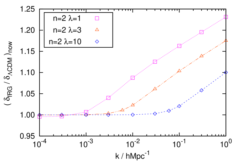
Figure 2: The ratio of linear density perturbations $\delta_{{\rm fRG}}/\delta_{{\rm\Lambda CDM}}$ at present as a function of $k$ for three different values of $\lambda$ with $n=2$.

In order to make a simple comparison of our results with observations of galaxy clustering, we define an effective wavenumber, $k_{\rm eff}(r)$, corresponding to each length scale $r$, in terms of the top-hat mass fluctuation within the same radius:

$$\sigma^{2}_{r}=\int\frac{d^{3}k}{(2\pi)^{3}}|W(kr)|^{2}P(k)\equiv\frac{4\pi k_{\rm eff}^{3}}{(2\pi)^{3}}P\left(k_{\rm eff}(r)\right),~{}~{}~{}W(kr)\equiv\frac{3j_{1}(kr)}{kr}.$$ (28)

Here $P(k)$ is the linear matter spectrum obtained by the standard CDM transfer functionEisenstein:1997ik with the scale-invariant initial power spectrum of perturbations, i.e. with the primordial spectral index $n_{s}=1$, and $W(kr)$ is the Fourier transform of the top-hat window function.

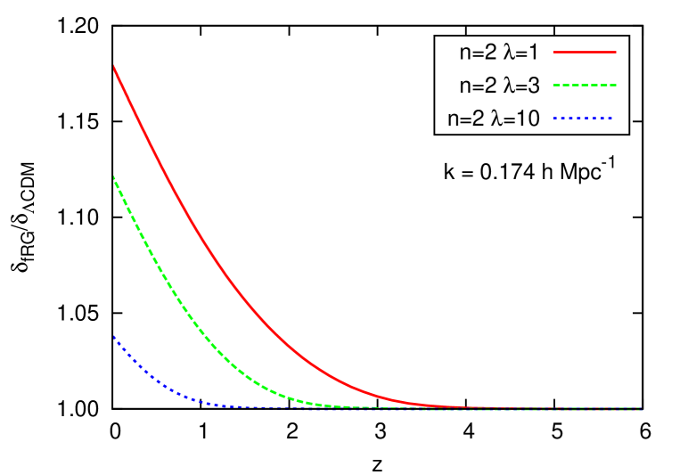
Figure 3: The ratio of linear density perturbations $\delta_{\rm fRG}/\delta_{{\rm\Lambda CDM}}(k=0.174h{\rm Mpc}^{-1}$) as a function of redshift for three different values of $\lambda$ with $n=2$.

The wavenumber of our particular interest is the scale corresponding to $\sigma_{8}$ normalization, for which we find $k_{\rm eff}(r=8h^{-1}{\rm Mpc})=0.174h{\rm Mpc}^{-1}$. Figure 3 depicts the redshift evolution of the ratio $\delta_{\rm fRG}/\delta_{{\rm\Lambda CDM}}$ for this scale for the same values of $n$ and $\lambda$ as in Fig. 2. Note that this ratio does not stop growing at the accelerated stage of the Universe expansion which begins at $z\approx 0.8$ for $\lambda=1$ and $z\approx 0.75$ for two other values of $\lambda$. Since the standard ${\rm\Lambda CDM}$ model normalized by large-scale CMB observations explains galaxy clustering at small scales well, $\delta_{{\rm fRG}}$ should not be too much larger than $\delta_{\rm\Lambda CDM}$ at these scales. We may typically require $(\delta_{{\rm fRG}}/\delta_{{\rm\Lambda CDM}})^{2}(k=0.174h{\rm Mpc}^{-1})\lesssim 1.1$. Although we neglect non-linear effects here, the difference between linear calculation and non-linear N-body simulation remained smaller than 5% at the wavenumber $0.174h{\rm Mpc}^{-1}$Oyaizu:2008tb .

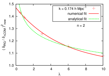
(a) $n=2$.

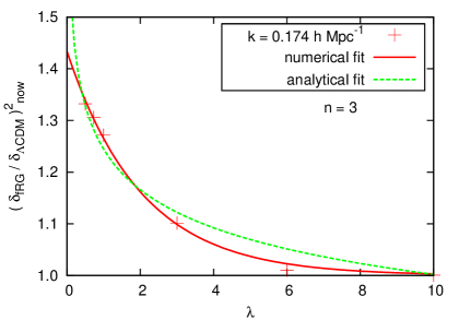
(b) $n=3$.

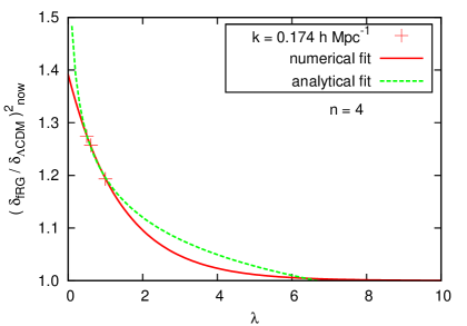
(c) $n=4$.

Figure 4: The present ratio $(\delta_{{\rm fRG}}/\delta_{{\rm\Lambda CDM}})^{2}(k=0.174h{\rm Mpc}^{-1})$ as a function of $\lambda$ together with two fitting functions.

Figures 4 represent $(\delta_{{\rm fRG}}/\delta_{{\rm\Lambda CDM}})^{2}(k=0.174h{\rm Mpc}^{-1})$ as a function of $\lambda$ for $n=2,3,$ and 4. From the analytic formula (19), this $\lambda$ dependence would have the form $(\delta_{{\rm fRG}}/\delta_{{\rm\Lambda CDM}})^{2}\propto C^{2}(k)\propto\lambda^{-\frac{(2n-p_{n}+1)(\sqrt{33}-5)}{4(3n+2)}}$ which is depicted by a broken line in each figure. This curve, however, does not match the asymptotic behaviour $(\delta_{{\rm fRG}}/\delta_{{\rm\Lambda CDM}})^{2}\longrightarrow 1$ for large $\lambda$. We find that an exponential function

$$(\delta_{{\rm fRG}}/\delta_{{\rm\Lambda CDM}})^{2}=1+b_{n}e^{-q_{n}\lambda}$$ (29)

fits the numerical calculation very well with $(n,b_{n},q_{n})=(2,0.47,0.19),~{}(3,0.43,0.49),$ and $(4,0.39,0.70)$ , respectively. From these figures, in order to keep deviation from ${\rm\Lambda CDM}$ model smaller than 10% at $k=0.174h{\rm Mpc}^{-1}$, we find $\lambda$ should be larger than 8.2, 3.0, and 1.9 for $n=2,3,$ and $4$, respectively.

From these analysis, we can constrain the parameter space as Fig. 5. The region which satisfy $(\delta_{{\rm fRG}}/\delta_{{\rm\Lambda CDM}})^{2}(k=0.174h{\rm Mpc}^{-1})<1.1$ corresponds to above the solid line. We also show the 20% boundary by the broken line. The region below the dotted line is forbidden because of instability of the de Sitter regime.

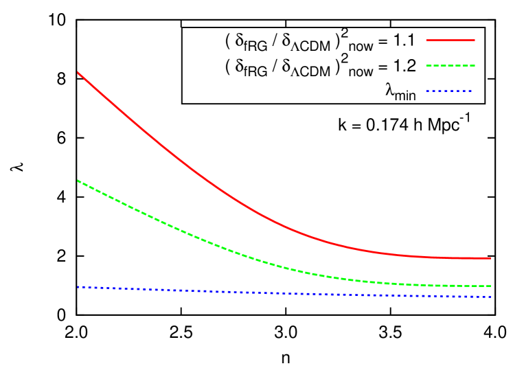
Figure 5: Constraints for parameter space.

Next we turn to another important quantity used to distinguish different theories of gravity, namely, the gravitational growth index, $\gamma(z)$, of density fluctuationsPeebles:1984ge ; Linder:2005in ; Polarski:2007rr ; Gannouji:2008wt ; Tsujikawa:2009ku ; Narikawa:2009ux . It is defined through

$$\frac{d\ln\delta}{d\ln a}=\Omega_{m}(z)^{\gamma(z)},~{}~{}~{}\text{or}~{}~{}~{}\gamma(z)=\frac{\log\left(\frac{\dot{\delta}}{H\delta}\right)}{\log\Omega_{m}}.$$ (30)

It takes a practically constant value $\gamma\cong 0.55$ in the standard ${\rm\Lambda CDM}$ modelPeebles:1984ge , but it evolves in time in modified gravity theories in general. We also note that $\gamma(z)$ has a nontrivial $k$-dependence in $f(R)$ gravity since density fluctuations with different wavenumbers evolve differently. Therefore, this quantity is a useful measure to distinguish modified gravity from the ${\rm\Lambda CDM}$ model in the Einstein gravity.

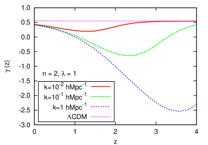
(a) Evolution of $\gamma(z)$ for $n=2$ $\lambda=1$.

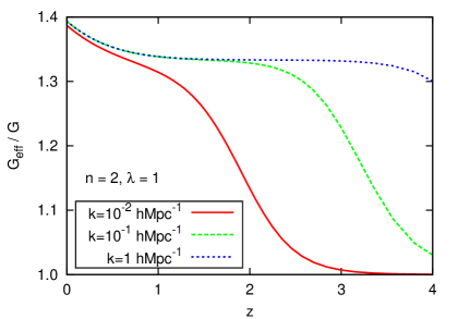
(b) Evolution of $G_{\text{eff}}/G$ for $n=2$ $\lambda=1$.

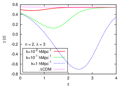
(c) Evolution of $\gamma(z)$ for $n=2$ $\lambda=3$.

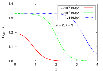
(d) Evolution of $G_{\text{eff}}/G$ for $n=2$ $\lambda=3$.

Figure 6: Evolution of $\gamma(z)$ and $G_{\text{eff}}/G$.

Figures 6 show evolution of $\gamma(z)$ together with that of $G_{\text{eff}}/G$ for different values of $k$. In the early high-redshift regime, $\gamma(z)$ takes a constant value identical to the ${\rm\Lambda CDM}$ model because $f(R)$ gravity is indistinguishable from the Einstein gravity plus a positive cosmological constant then. It gradually decreases in time, reaches a minimum, and then increase again towards the present epoch. We can understand this tendency from the evolution equation for $\gamma(z)$Polarski:2007rr ,

$$- (1+z)\ln(1-\Omega_{\rm DE})\frac{d\gamma}{dz}$$

$$=-(1-\Omega_{\rm DE})^{\gamma}-\frac{1}{2}\left[1+3(2\gamma-1)w_{\rm DE}\Omega_{\rm DE}\right]+\frac{3}{2}\frac{G_{\text{eff}}}{G}(1-\Omega_{\rm DE})^{1-\gamma},$$ (31)

where $\Omega_{\rm DE}=1-\Omega_{m}$ is the density parameter of dark energy based on (8). In the high-redshift era when $\Omega_{\rm DE}$ is small, the above equation may be approximated as

$$(1+z)\Omega_{\rm DE}\frac{d\gamma}{dz}$$

$$=\frac{3}{2}\left(\frac{G_{\text{eff}}}{G}-1\right)+\Omega_{\rm DE}\left[\frac{11}{2}\left(\gamma-\frac{6}{11}\right)-\frac{3}{2}(1-\gamma)\left(\frac{G_{\text{eff}}}{G}-1\right)-\frac{3}{2}(2\gamma-1)(w_{\rm DE}+1)\right].$$ (32)

In the earlier stage, the first term in the right-hand side is more important. That explains why $\gamma(z)$ starts to decrease when $G_{\text{eff}}/G$ starts to increase. As time goes by towards lower redshifts, the second term becomes more important to make $\gamma(z)$ increase again. We note that recently Narikawa and YamamotoNarikawa:2009ux calculated time evolution of $\gamma(z)$ in a simplified model (15) numerically and also obtained some analytic expansion, which behaves qualitatively the same as our numerical results but with much more exaggerated amplitudes. Our results, which satisfy all the viability conditions, exhibit milder deviation from the ${\rm\Lambda CDM}$ model than those they found. Existing constraints on the growth indexRapetti:2009ri are not strong enough to detect any deviation from the ${\rm\Lambda CDM}$ model and/or to obtain new bounds on $f(R)$ DE models, but future observations may reveal its time and wavenumber dependence.

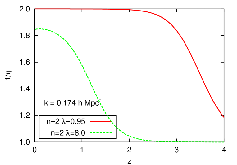
Figure 7: The evolution of $1/\eta=\Phi/\Psi$ with $n=2$.

Another quantity which can characterize the evolution of density perturbations more directly is the ratio $\delta_{{\rm fRG}}(z=0.5)/\delta_{{\rm fRG}}(z=0)$. However, it varies only from 0.75 to 0.78 for different choices of the model parameters when the current matter density parameter is fixed to $\Omega_{m0}=0.27$ and $n\geq 2$. This variation is smaller than that caused by the uncertainty of $\Omega_{m0}$Gannouji:2008wt . So, at present it does not help much to single out the best DE model among the considered ones, in contrast to the $f(R)$ DE modelHu:2007nk (it has the same behaviour (15) for $R\gg R_{s}$) in the case corresponding to $n=0.5$ in our notations which was recently studied in Ref. SVH09 .

Finally we consider the quantity $1/\eta=\Phi/\Psi$, namely the ratio of gravitational potential to curvature perturbation, for which some results from observational data were recently obtained in Ref. Bean:2009wj . In $f(R)$ gravity, $1/\eta$ is expressed as

$$\frac{1}{\eta}=2-\frac{1}{1+2\frac{k^{2}}{a^{2}}\frac{F^{\prime}}{F}}.$$ (33)

Due to the stability conditions $F>0,~{}F^{\prime}>0$, this quantity always lies between 1 and 2. Thus, stable $f(R)$ DE models may not explain such a large value of $1/\eta$ which is presented in Ref. Bean:2009wj for the redshift interval $1<z<2$. Figure 7 shows the evolution of $1/\eta$ for $n=2$ and $\lambda=0.95$ (the minimal possible value) and $8$.

IV Conclusions

In the present paper we have numerically calculated the evolution of both homogeneous background and density fluctuations in a viable $f(R)$ DE model based on the specific functional form proposed in Ref. Starobinsky:2007hu . We have found that viable $f(R)$ gravity models of present DE and accelerated expansion of the Universe generically exhibit phantom behaviour during the matter-dominated stage with crossing of the phantom boundary $w_{\rm DE}=-1$ at redshifts $z\lesssim 1$. The predicted time evolution of $w_{\rm DE}$ has qualitatively the same behaviour as that was recently obtained from observational data in Ref. Shafieloo:2009ti . However, it is important that the condition of stability, or even metastability, of the future de Sitter epoch strongly restricts possible deviation of $w_{\rm DE}$ from $-1$ by several percents in these models. Thus, the DE phantomness should be small, if exists at all, that agrees with present observational data. Still for the models considered, it is not so hopelessly small as in the case of the similar modelHu:2007nk with $n=0.5$ recently considered in Ref. SVH09 using data on cluster abundance. Note also, that in contrast to Ref. BBDS08 , we do not impose the so called thin-shell condition $|\Delta(f^{\prime}(R)-1)|\lesssim|\Phi_{N}|$, where $\Phi_{N}$ is the Newtonian potential of matter inhomogeneities and $\Delta$ means change in the quantity in question, for scales exceeding galatic ones where a background matter density approaches the cosmological one. On the other hand, this condition is satisfied automatically for matter overdensities more than $10$ for the parameter range $n\geq 2$ considered in our paper.

As for the density fluctuations, we have numerically confirmed our previous analytic results of a shift in the power spectrum index for larger wavenumbers which exceed the scalaron mass during the matter-dominated epochMotohashi:2009qn , while for smaller wavenumbers fluctuations have the same amplitude as in the ${\rm\Lambda CDM}$ model. Once more, the future de Sitter epoch stability condition bounds possible increase in density fluctuations for cluster scales (compared to the ${\rm\Lambda CDM}$ model) by $\sim 20\%$ for $n\geq 2$. On the contrary, if it is proven from observational data that this increase is less than $5\%$, then the background evolution should be practically indistinguishable from the ${\rm\Lambda CDM}$ one: $|w_{\rm DE}+1|<10^{-4}$ for $n=2$. This shows that $\sigma_{8}$ and related density perturbations tests are the most critical ones for the $f(R)$ DE models considered in the paper. We have obtained that the upper limit on $|w_{\rm DE}+1|$ for $n=2$ and $\lambda=8$ is $4.4\times 10^{-5}$ when $z=0.16$, which is of the same order as $B(0)$.

We have also investigated the growth index $\gamma(k,z)$ of density fluctuations and have presented an explanation of its anomalous evolution in terms of time dependence of $G_{\text{eff}}$. Since $\gamma$ has characteristic time and wavenumber dependence, future detailed observations may yield useful information on the validity of $f(R)$ gravity through this quantity, although current constraints have been obtained assuming that it is constant both in time and in wavenumberBean:2009wj ; Rapetti:2009ri . Another related observational test of this model is supplied by the large-scale structure of the Universe which should be different from that in the ${\rm\Lambda CDM}$ model. In particular, voids are expected to be more pronounced since the effective gravitational constant is bigger inside them compared to large matter overdensities where it is practically equal to that measured in laboratory.

- (1) V. Sahni and A. A. Starobinsky, Int. J. Mod. Phys. D 9, 373 (2000) [arXiv:astro-ph/9904398]; P. J. E. Peebles and B. Ratra, Rev. Mod. Phys. 75, 559 (2003) [arXiv:astro-ph/0207347]; T. Padmanabhan, Phys. Rept. 380, 235 (2003) [arXiv:hep-th/0212290]; V. Sahni, Lect. Notes Phys. 653, 141 (2004) [arXiv:astro-ph/0403324]; E. J. Copeland, M. Sami and S. Tsujikawa, Int. J. Mod. Phys. D 15, 1753 (2006) [arXiv:hep-th/0603057]; V. Sahni and A. A. Starobinsky, Int. J. Mod. Phys. D 15, 2105 (2006) [arXiv:astro-ph/0610026].
- (2) E. Komatsu et al., arXiv:1001.4538 [astro-ph.CO].
- (3) A. Shafieloo, V. Sahni and A. A. Starobinsky, Phys. Rev. D 80, 101301 (R) (2009) [arXiv:0903.5141 [astro-ph.CO]].
- (4) R. Bean, arXiv:0909.3853 [astro-ph.CO].
- (5) J. Yokoyama, Phys. Rev. Lett. 88, 151302 (2002) [arXiv:hep-th/0110137].
- (6) A. A. Starobinsky, Phys. Lett. 91B, 99 (1980).
- (7) K. Sato, Mon. Not. Roy. Astron. Soc. 195, 467 (1981).
- (8) A. H. Guth, Phys. Rev. D 23, 347 (1981).
- (9) T. P. Sotiriou and V. Faraoni, arXiv:0805.1726 [gr-qc].
- (10) T. Chiba, Phys. Lett. B 575, 1 (2003) [arXiv:astro-ph/0307338].
- (11) S. Tsujikawa, K. Uddin, S. Mizuno, R. Tavakol and J. Yokoyama, Phys. Rev. D 77, 103009 (2008) [arXiv:0803.1106 [astro-ph]].
- (12) W. Hu and I. Sawicki, Phys. Rev. D 76, 064004 (2007) [arXiv:0705.1158 [astro-ph]].
- (13) A. Appleby and R. Battye, Phys. Lett. B 654, 7 (2007) [arXiv:0705.3199 [astro-ph]].
- (14) A. A. Starobinsky, JETP Lett. 86, 157 (2007) [arXiv:0706.2041 [astro-ph]].
- (15) H. Motohashi, A. A. Starobinsky and J. Yokoyama, Int. J. Mod. Phys. D 18, 1731 (2009) [arXiv:0905.0730 [astro-ph.CO]].
- (16) A. V. Frolov, Phys. Rev. Lett. 101, 061103 (2008) [arXiv:0803.2500 [astro-ph]].
- (17) I. Thongkool, M. Sami and S. Rai Choudhury, Phys. Rev. D 80, 127501 (2009) [arXiv:0908.1693 [ge-qc]].
- (18) S. Appleby, R. Battye and A. Starobinsky, arXiv:0909.1737 [astro-ph.CO].
- (19) A. Dev et al., Phys. Rev. D 78, 083515 (2008) [arXiv:0807.3445 [hep-th]].
- (20) T. Kobayashi and K. Maeda, Phys. Rev. D 79, 024009 (2009) [arXiv:0810.5664 [astro-ph]].
- (21) V. F. Mukhanov and G. V. Chibisov, JETP Lett. 33, 532 (1981).
- (22) A. A. Starobinsky, Sov. Astron. Lett. 9, 302 (1983).
- (23) B. Boisseau, G. Esposito-Farese, D. Polarski and A. A. Starobinsky, Phys. Rev. Lett. 85, 2236 (2000) [arXiv:gr-qc/0001066].
- (24) V. Müller, H.-J. Schmidt and A. A. Starobinsky, Phys. Lett. B 202, 198 (1988).
- (25) M. Chevallier and D. Polarski, Int. J. Mod. Phys. D 10, 213 (2001) [arXiv:gr-qc/0009008]; E. V. Linder, Phys. Rev. Lett. 90, 091301 (2003) [arXiv:astro-ph/0208512].
- (26) M. Martinelli, A. Melchiorri and L. Amendola, Phys. Rev. D 79, 123516 (2009) [arXiv:0906.2350 [astro-ph.CO]].
- (27) L. Amendola and S. Tsujikawa, Phys. Lett. B 660, 125 (2008) [arXiv:0705.0396 [astro-ph]]; S. Tsujikawa, Phys. Rev. D 77, 023507 (2008) [arXiv:0709.1391 [astro-ph]].
- (28) Y. S. Song, W. Hu and I. Sawicki, Phys. Rev. D 75, 044004 (2007) [arXiv:astro-ph/0610532].
- (29) P. Zhang, Phys. Rev. D 73, 123504 (2006) [arXiv:astro-ph/0511218].
- (30) S. Tsujikawa, Phys. Rev. D 76, 023514 (2007) [arXiv:0705.1032 [astro-ph]].
- (31) J. M. Bardeen, J. R. Bond, N. Kaiser and A. S. Szalay, Astrophys. J. 304, 15 (1986); D. J. Eisenstein and W. Hu, Astrophys. J. 496, 605 (1998) [arXiv:astro-ph/9709112].
- (32) H. Oyaizu, M. Lima and W. Hu, Phys. Rev. D 78, 123524 (2008) [arXiv:0807.2462 [astro-ph]].
- (33) R. Gannouji, B. Moraes and D. Polarski, JCAP 0902, 034 (2009) [arXiv:0809.3374 [astro-ph]].
- (34) P. J. E. Peebles, Astrophys. J. 284, 439 (1984).
- (35) E. V. Linder, Phys. Rev. D 72, 043529 (2005) [arXiv:astro-ph/0507263]; Phys. Rev. D 79, 063519 (2009) [arXiv:0901.0918 [astro-ph.CO]].
- (36) D. Polarski and R. Gannouji, Phys. Lett. B 660, 439 (2008) [arXiv:0710.1510 [astro-ph]].
- (37) S. Tsujikawa, R. Gannouji, B. Moraes and D. Polarski, Phys. Rev. D 80, 084044 (2009) [arXiv:0908.2669 [astro-ph.CO]].
- (38) T. Narikawa and K. Yamamoto, arXiv:0912.1445 [astro-ph.CO].
- (39) D. Rapetti, S. W. Allen, A. Mantz and H. Ebeling, arXiv:0911.1787 [astro-ph.CO].
- (40) F. Schmidt, A. Vikhlinin and W. Hu, Phys. Rev. D 80, 083505 (2009) [arXiv:0908.2457 [astro-ph.CO]].
- (41) P. Brax, C. van de Bruck, A.-C. Davis and D. J. Shaw, Phys. Rev. D 78, 104021 (2008) [arXiv:0806.3415 [astro-ph]].