A Stochastic Local Search algorithm for distance-based phylogeny reconstruction

Abstract

In many interesting cases the reconstruction of a correct phylogeny is blurred by high mutation rates and/or horizontal transfer events. As a consequence a divergence arises between the true evolutionary distances and the differences between pairs of taxa as inferred from available data, making the phylogenetic reconstruction a challenging problem. Mathematically this divergence translates in a loss of additivity of the actual distances between taxa. In distance-based reconstruction methods, two properties of additive distances were extensively exploited as antagonist criteria to drive phylogeny reconstruction: on the one hand a local property of quartets, i.e., sets of four taxa in a tree, the four-points condition; on the other hand a recently proposed formula that allows to write the tree length as a function of the distances between taxa, the Pauplin’s formula. Here we introduce a new reconstruction scheme, that exploits in a unified framework both the four-points condition and the Pauplin’s formula. We propose, in particular, a new general class of distance-based Stochastic Local Search algorithms, which reduces in a limit case to the minimization of the Pauplin’s length. When tested on artificially generated phylogenies our Stochastic Big-Quartet Swapping algorithmic scheme significantly outperforms state-of-art distance-based algorithms in cases of deviation from additivity due to high rate of back mutations. A significant improvement is also observed with respect to the state-of-art algorithms in case of high rate of horizontal transfer.

I Introduction

Phylogenetic methods have recently been rediscovered in several interesting areas among which immunodynamics, epidemiology and many branches of evolutionary dynamics. The reconstruction of phylogenetic trees belongs to a general class of inverse problems whose relevance is now well established in many different disciplines ranging from biology to linguistics and social sciences Gray and Atkinson (2003); Lazer et al. (2009); Pybus and Rambaut (2009); Liu et al. (2009). In a generic inverse problem one is given with a set of data and has to infer the most likely dynamical evolution process that presumably produced the given data set. The relevance of inverse problems has been certainly triggered by the fast progress in data-revealing technologies. In molecular biology, for instance, a great amount of genomes data are available thanks to the new high-throughput methods for genome analysis Ragoussis (2009). In historical linguistics Renfrew et al. (2000) a remarkable effort has been recently done for the compilation of corpora of homologous features (lexical, phonological, syntactic) or characters for many different languages.

Although phylogenetic reconstruction is not a novel topic, dealing with not purely tree-like processes and identifying the possible sources of non-additivity and their effects in a given dataset is still an open and challenging problem Felsenstein (2004); Gascuel ed. (2007).

Here we focus on distance-based methods Cavalli-Sforza and Edwards (1967); Fitch and Margoliash (1967) and investigate how deviations from additivity affect their performances. In distance-based methods only distances between leaves are considered, and all the information possibly encoded in the combinatorial structure of the character states is lost. Despite their simplicity, distance-based methods are still widely used thanks to their computational efficiency, but a solid theoretical understanding on the limitation of their applicability is still lacking. One of the most popular distance-based reconstruction algorithm, Neighbor-Joining (NJ) Saitou and Nei (1987), was proposed in the late 80’s, but it is only recently that its theoretical background was put on a more solid basis Atteson (1997); Gascuel and Steel (2006); Mihaescu et al. (2007). Another step toward a better understanding of distance-based methods was obtained thanks to an interesting property of additive distances, the Pauplin’s formula Pauplin (2000). This property has been used in the formulation of a novel algorithmic strategy with improved performances (FastME) Desper and Gascuel (2002). In parallel, another fundamental property of additive trees, the four-points condition Gusfield (1997), has been extensively exploited in distance-based phylogenetic reconstruction methods Erdös et al. (1998); Snir et al. (2008). Both the Pauplin’s formula and the four-points condition will be discussed in details below.

Here we propose a new approach that combines the four-points condition and the Pauplin’s formula in a Stochastic Local Search (SLS) scheme that we name Stochastic Big-Quartet Swapping (SBiX) algorithm. SLS Hoos and Stützle (2005) algorithms transverse the search space of a given problem in a systematic way, allowing for a sampling of low cost configurations. SLS algorithms start from a randomly chosen initial condition. Subsequently the elementary step is a move from a configuration to a neighboring one. Each move is determined by a decision based on local knowledge only. Typically the decision is taken combining, with a given a priori probability, a greedy step (i.e., a step that reduces the local cost contribution), with a random one where the local cost is not taken into account. SLS algorithms have been widely used in solving complex combinatorial optimization problems such as Satisfiability, Coloring, MAX-SAT, and Traveling Salesman Problem Hoos and Stützle (2005).

At the heart of our new algorithmic scheme (named SBiX) there is the notion of quartet frustration, a quantitative measure of how good a given configuration is, in the space of trees. Following a concept already introduced in Snir et al. (2008), we weight the different quartets according to their length, in order to reduce the effect of those which are more likely to undergo double mutations. The strength of our approach comes from a combination of this strategy with a Pauplin’s like one, weighting each quartet according to a purely topological property.

We tested the performances of the proposed reconstruction algorithm, i.e., the ability to reconstruct the true topology, in the presence of high levels of deviation from additivity due to both horizontal transfer and back-mutation processes. We use both a very simple model to generate artificial phylogenies of binary sequences, and the more realistic Kimura two-parameters model, considering sequences with $q$-state sites, with $q=4$. We have evidence that the performance of our algorithm does not rely on the particular evolutive process giving rise to the phylogeny, nor on the particular representation of the taxa. We find that when the lack of additivity arises from high mutation rates (and consequently high probability of back mutations), our algorithm significantly outperforms the state-of-art distance-based algorithms. When the lack of additivity arises from high rate of horizontal transfer events, our algorithm performs better than the algorithms we considered as competing ones.

We show results both for a greedy and a simulated-annealing-like strategy of our algorithm, the former being significantly faster than the latter and with comparable performances. The SBiX algorithm has a complexity of $O(N^{4})$, which is higher that the one of the distance-based algorithms used as competitors for comparing the performances. Nevertheless, the prefactor of the greedy version is so low that our algorithm is fast enough to reconstruct large phylogenies e.g., of a few thousands taxa, in a time remarkably slower with respect to any character based reconstruction algorithm. A comparison of the running time and of the performances of our algorithm with a popular character based one, MrBayes Huelsenbeck and Ronquist (2001), is reported respectively in the Appendix II and in the section Results. We show that, while the performances of the two algorithms are comparable, the running time of MrBayes greatly exceed ours, becoming comparable when the reconstruction becomes in practise unfeasible, that is for running times of the order of some thousand of years, and number of taxa of the order of one hundred thousand.

II Methods

II.1 Additivity and the four-points condition

A distance matrix is said to be additive if it can be constructed as the sum of a tree’s branches lengths. Two fundamental and widely used properties of additive distances are the Pauplin’s formula Pauplin (2000) and the four-points condition Gusfield (1997). For the sake of clarity, we recall them here.

Given any quadruplet of taxa $a,b,c,d$, let $D_{1}=d(a,b)+d(c,d)$, $D_{2}=d(a,c)+d(b,d)$, and $D_{3}=d(a,d)+d(b,c)$ be the three possible pairs of distances between the four taxa. A matrix $M$ is additive if and only if $D_{1}<D_{2}=D_{3}$ or $D_{2}<D_{1}=D_{3}$ or $D_{3}<D_{1}=D_{2}$. When considering experimental data, additivity is almost always violated and so is the four-points condition. In order to set up a robust method for phylogeny reconstruction based on the four-points condition, we need to relax the notion of additivity and to quantify violations in a suitable way. For any four taxa $a,b,c,d$ such that $a,b$ are on one side of the tree and $c,d$ on the other (as in fig. 1), the quartet $(ab:cd)$ is said to satisfy the weak four-points condition if $D_{1}=\min(D_{1},D_{2},D_{3})$ (where $D_{1},D_{2},D_{3}$ are defined as above). It is easy to prove that if the distance matrix $M$ is additive a unique tree exists in which all quartets satisfy the weak four-points condition and this tree is the correct one. Many algorithms have been proposed that exploit this weak four-points condition, one of the most promising being, for instance, the short-quartet method Erdös et al. (1998); Snir et al. (2008).

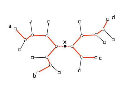
Figure 1: Quartet definition. The quartet $a,b,c,d$ induces an internal edge $x$ that divides the tree in two parts. All paths joining any pair of sites sitting on opposite parts of the tree pass through $x$.

II.2 Pauplin’s distance

Another remarkable property of an additive tree is the possibility to compute its total length $L$, defined as the sum of all its branches lengths, through a formula, due to Pauplin Pauplin (2000), that only uses distances between taxa:

$$L_{P}=\sum_{a<b}2^{-t(a,b)}M(a,b),$$ (1)

where $t(a,b)$ is the number of nodes on the path connecting $a$ and $b$, i.e., their topological distance. For additive trees $L\equiv L_{P}$, but even when the four-points condition is no longer satisfied, $L_{P}$ is a particularly good approximation for the tree length Desper and Gascuel (2002). Furthermore, it is recognized that for distance matrices sufficiently “close” to additivity Atteson (1997) the correct phylogeny minimizes $L_{P}$ Mihaescu et al. (2007); Bordewich et al. (2009). This principle is used in an implicit way in Neighbor-Joining Saitou and Nei (1987) and more explicitly in a new generation distance-based algorithm, FastME Desper and Gascuel (2002). When departure from additivity is too strong $L_{P}$ is no longer a good functional to minimize in order to recover the correct tree.

II.3 Violations of additivity

Violations of additivity can arise both from experimental noise and from properties of the evolutionary process the data come from. We here consider two of the main sources of violations of the latter type that can either occur together or singularly. (i) back-mutation: in particularly long phylogenies, here the time-scale being set by the mutation rate, a single character can experience multiple mutations. In this case the distances between taxa are no longer proportional to their evolutionary distances; we will use in the following the expression back-mutation as synonymous of multiple mutation on the same site; (ii) horizontal transfer: the reconstruction of a phylogeny from data underlies the assumption that information flows vertically from ancestors to offsprings. However, in many processes information flows also horizontally. Horizontal (or lateral) gene transfers Simonson et al. (2005) are often well known confounding factors for a correct phylogenetic inference.

II.4 The Stochastic Big-Quartet Swapping algorithm

Here we describe the structure of our Stochastic Big-Quartet Swapping (SBiX) algorithm. As already mentioned this algorithm crucially exploits both the weak four-points condition and the Pauplin’s distance, featuring a larger robustness with respect to violations of additivity if compared to algorithms based separately on the weak four-points condition or on the minimization of the Pauplin’s length.

The general structure of the SBiX algorithm is as follows:

• start with a tree topology for the given set of taxa;

• update the tree topology by local elementary rearrangements through sub-trees quartet swapping;

• repeat point $2$ till convergence is reached;

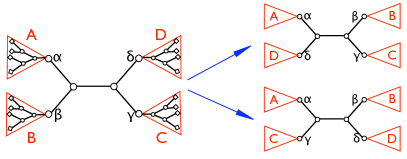
Figure 2: Elementary move of our Stochastic Local Search scheme. Any internal edge defines the four subtrees $A,B,C,D$ rooted respectively on $\alpha,\beta,\gamma,\delta$. Here, the initial reference configuration $((A,B),(C,D))$ displayed on the left, leads to two possible rewiring: (i) swap the pair $B\leftrightarrow D$ (right-upper panel), (ii) swap the pair $B\leftrightarrow C$ (right-lower panel).

II.5 Sub-trees (big-)quartets swaps

We analyze the three points in details in the following:

• In the simulated-annealing-like version of the algorithm we start with a random topology. In the greedy version we search for a local minimum (which can eventually be the global one), so it is important to start with a meaningful topology. We tested the algorithm starting both with the FastME and the NJ reconstructed topologies.

• We sequentially consider all the internal edges of the present topology. Each internal edge defines four subtrees (see fig. 2), say $A,B,C,D$, rooted respectively on the four internal nodes $\alpha,\beta,\gamma,\delta$. Referring to fig. 2, let $((A,B),(C,D))$ being the initial configuration. We randomly choose one of the two possible local rewirings: (i) swap the pair $B\leftrightarrow D$ getting the configuration $((A,D),(B,C))$, (ii) swap the pair $B\leftrightarrow C$ getting the configuration $((A,C),(B,D))$. In the simulated-annealing version, the new configuration is accepted with a probability proportional to the statistical weight $e^{-\beta\mathrm{sign}(\Delta E)}$ where $\beta$ is an inverse temperature-like parameter that is set by a simulated annealing-like Kirkpatrick et al. (1983) strategy and $\Delta E$ is the difference of the two configurations local costs: for case (i) $\Delta E=E_{((A,D),(B,C))}-E_{((A,B),(C,D))}$ while for case (ii) $\Delta E=E_{((A,C),(B,D))}-E_{((A,B),(C,D))}$. In the greedy (or zero temperature) version, the new configuration is accepted if and only if $\Delta E<0$.

• In the simulated-annealing version, we iterate point $2$ starting with $\beta=0$ and increasing it at a constant rate at each sweep (where we call sweep an update of all the internal edges) until convergence is reached, i.e., until the algorithm gets stuck in a fixed topology. In the greedy version, we iterate point $2$ until the algorithm gets stuck in a fixed topology.

In order to define the configurational local cost, say $E_{((A,B),(C,D))}$, we consider all the quartets $(ab:cd)$ such that $a\in A$ ($a$ is a taxa of the subtree $A$) , $b\in B$, $c\in C$, and $d\in D$. For each quartet we define the quartet frustration as:

$$f_{(ab:cd)}=\max\left(0,\frac{D_{1}-\min(D_{2},D_{3})}{(D_{1}+\min(D_{2},D_{3}))^{k}}\right),$$ (2)

where $D_{1},D_{2},D_{3}$ are the sums of distances already defined ($D_{1}=d(a,b)+d(c,d)$, $D_{2}=d(a,c)+d(b,d)$, $D_{3}=d(a,d)+d(b,c)$). The normalization factor in the right-hand side of Eq. 2, as already pointed out in the introduction, gives a smaller weight to longer distances, typically affected by noise and recombination. The parameter fixing strategy for the exponent $k$ will be discussed in the next subsection.

The cost $E_{((A,B),(C,D))}$ of the configuration $((A,B),(C,D))$ is thus defined as the sum of the costs (frustrations) of all the considered quartets, each weighted with a factor borrowed from the Pauplin’s formula:

$$E_{((A,B),(C,D))}=\sum_{(ab:cd)}f_{(ab:cd)}2^{-t(a,\alpha)-t(b,\beta)-t(c,\gamma)-t(d,\delta)},$$ (3)

where $t(a,\alpha)$ is the topological distance between the taxa $a$ and the internal node $\alpha$, and analogously for the other taxa.

II.6 Remarks on the cost definition

When $k=0$ in Eq. 2 our procedure is equivalent to the minimization of the Pauplin’s length (the proof of this statement will be discussed in the Appendix IA). On the other hand, if the Pauplin weights $2^{-t(a,\alpha)}$, $2^{-t(b,\beta)}$, $2^{-t(c,\gamma)}$, $2^{-t(d,\delta)}$ were absent, the difference in local costs between two configurations would be equal to the variation of a global cost, defined as $E=\sum_{(abcd)}f_{(ab:cd)}$. Here the sum defining the cost, $\sum_{(abcd)}$, is running over all the quartets of the tree and not only on the quartets compatible with the sub-trees $A,B,C,D$. We will refer to our algorithm with this form of the cost configuration as the Normalized Quartets method (NQ).

Conversely, when one takes the complete form of the local cost as defined in Eq. 3, with $k>0$ in Eq. 2, the local cost differences do not correspond to any global cost difference (the proof of this statement will be discussed in Appendix IB). It is however an open question whether a global functional can be defined whose variation between each pair of configurations is compatible with the sign of our local cost difference.

The complexity of a sweep of our algorithm (i.e., $N$ configurations updates, where $N$ is the number of leaves in the tree), has a leading term $O(N^{4})$. The number of quartets to be considered when updating all the edges of the tree in case of a perfectly balanced tree reads:

$${\cal N}=\frac{85}{5376}N^{4}-\frac{N^{2}}{3}+\frac{4}{7}N\,.$$ (4)

. We show the results of numerical simulations for the running time of the greedy version of our algorithm in Appendix IIB. If considering the Normalized Quartets method, a naïve minimization of the corresponding functional would lead to a complexity of $O(N^{5})$, while a Montecarlo sweep for a naïve minimization of the Pauplin length is only $O(N^{3})$. Despite the $O(N^{4})$ complexity of the SBiX algorithm, the greedy version has an extremely low prefactor, making the algorithm suitable for trees with a large number of taxa (see Appendix IIB).

III Results

III.1 Artificial phylogenies

To test the performances of our algorithm, we consider artificially generated phylogenies following one of the simplest evolutionary model that takes into account both mutational events and horizontal transfer. Each taxon is represented by a binary sequence of length $l$. We start with one sequence, for instance the sequence with all the bits equal to $0$. Then at each time step we perform the following operations: (i) we randomly extract one of the already existing leaf sequences, say $\bar{s}$; (ii) with probability $\tau$ a randomly extracted portion of length $l/4$ of $\bar{s}$ is replaced with the corresponding portion of another randomly chosen sequence ; (iii) $\bar{s}$ generates two clones as descendants; (iv) each site of the two new sequences is independently flipped with probability $m/l$, where $m$ is extracted from an exponential distribution with average $\mu$ (average number of mutations per sequence per time step). To ensure that at least on site mutates at each branching event, we randomly choose a site to mutate if no site mutated. We iterate this procedure until the desired number of taxa is obtained.

We here consider as distance between two taxa the correct hamming distance Felsenstein (2004), defined as:

$$d_{corr}=-\frac{1}{2}\ln(1-2h),$$ (5)

where $h$ is the hamming distance, defined as the fraction of sites in which the sequences differ.

Although the evolutionary model described above is a toy model for describing evolution, it allows to control and to tune noise as well as horizontal transfer events. We also test our algorithm on phylogenies constructed following more realistic model of evolution, such us the standard $4$-states two parameters Kimura model Kimura, M. (1980). In particular, we follow the same steps described above for the $2$-state model, but we now consider sequences of nucleotides, with an alphabet of $4$ letters, and different rates of transitions ($\alpha$) and transversions ($2\beta$). We consider in this case as distance between two taxa the correct hamming distance for the Jukes-Cantor model Felsenstein (2004) that is the limit of the Kimura model when $\alpha=\beta$, which reads:

$$d^{\mathrm{JC}}_{corr}=-\frac{3}{4}\ln(1-\frac{4}{3}h).$$ (6)

III.2 Robinson-Foulds measure

In order to assess the performances of the different algorithms to reconstruct the true phylogeny, we consider the standard Robinson-Foulds measure (RF) Robinson and Foulds (1981), which counts the number of bipartitions on which the inferred tree differs from the true one. A bipartition is a split of the leaves in two sets realized through a cut of a tree edge. We recall that it exists a one-to-one correspondence between the bipartitions of the tree and the set of its edges, so that each tree is uniquely characterized by the set of bipartitions it induces. Note that, since we consider only binary trees, the number of true positive bipartitions equals the number of false positive bipartitions and both are equal to the RF measure.

III.3 Competing algorithms

In order to assess the performances of our algorithm, both in its simulated annealing and greedy version, we compare it with the Neighbor-Joining (NJ) Saitou and Nei (1987) and the FastME Desper and Gascuel (2002) algorithms. In addition we implemented the Pauplin’s length minimization (from now onwards referred as PAUPLIN) by making use of our SBiX algorithm in its form with $k=0$ (see above the section about the algorithm’s description). This in order to directly investigate the effectiveness of a non-greedy minimization of the Pauplin’s length in reconstructing trees. Finally we implemented the version of our algorithm without the Pauplin’s weights (NQ) (as discussed above). We also show a comparison with the performances of a state-of-the-art character based algorithm, MrBayes Huelsenbeck and Ronquist (2001).

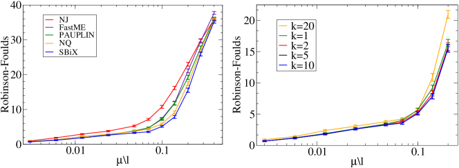
Figure 3: Performances comparison as a function of the mutation rate. Left: Robinson-Foulds distance between the reconstructed and the true trees as a function of the mutation rate per site of the generative evolutionary model. The horizontal transfer rate $\tau$ is here kept $\tau=0$. We compare the performances of the SBiX algorithm with $k=5$ with: Neighbor-Joining (NJ), FastME, the Pauplin length minimization (PAUPLIN), and Normalized-Quartets (NQ). Right: dependence of the SBiX algorithm on the parameter $k$. The best performances are very stable in the range of $k$ between $5$ and $10$. In both figures results are averaged over $100$ independent realizations for each reported mutation rate. The error bars are standard errors. All the trees generated have $N=60$ leaves and the sequences have fixed length $l=1000$.

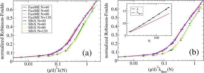
Figure 4: System-size dependence. Behavior of the normalized Robinson-Foulds distance for the SBiX algorithm and FastME for different system sizes, i.e., different values $N$ of the number of leaves. Here normalized means the Robinson-Foulds distance divided by its maximal value $N-3$. In all the cases curves for different values of $N$ collapse as a function of $\mu^{2}\lambda(N)$ (see text for details) where $\lambda(N)$ is the average distance between two leaves in a tree with $N$ leaves. In both the analysis the horizontal transfer rate $\tau$ is kept $\tau=0$. We use both the true value of $\lambda(N)$ in the simulated phylogenies (a), and the value analytically calculated in the case of perfectly balanced trees $\lambda_{\mathrm{theo}}(N)$ (b). In the inset of (b) we report the behavior of $\lambda$ and $\lambda_{\mathrm{theo}}$ as a function of tree size $N$. The experimental values $\lambda(N)$ are systematically larger than $\lambda_{\mathrm{theo}}$ putting in evidence a slight deviation of the generated trees from a perfectly balance condition.

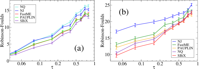
Figure 5: Performances comparison as a function of the horizontal transfer rate. Robinson-Foulds measure for the reconstructed trees as a function of the horizontal transfer rate of the generative model. We compare the performances of our SBiX algorithm (with $k=5$) with those of the following ones: Neighbor-Joining (NJ), FastME, the Pauplin length minimization algorithm (PAUPLIN) and the Normalized-Quartet (NQ) algorithm. Results are averages over $100$ independent realizations for each reported horizontal transfer rate. The error bars are standard errors. All the trees generated have $N=60$ leaves. (a): mutation rate per site $\mu/l=0.003$ while the sequences have fixed length $l=10000$. (b): mutation rate per site of $\mu/l=0.14$ while the sequences have fixed length $l=1000$.

III.4 Performances of the different algorithms

In this section we compare the performances of all the considered algorithms as a function of the mutation rate and of the horizontal transfer rate in the underlying evolutionary process described in the previous subsection.

In fig. 3 we show the Robinson-Foulds curves for different algorithms (Left) as a function of the mutation rate for a fixed tree size ($N=60$) and $k=5$. In the whole range of values of the mutation rate all the versions of our algorithm (PAUPLIN, NQ and SBiX) outperforms both NJ and FastME. In particular SBiX outperforms all the other algorithms. Differences between the global minimization of the Pauplin’s length (PAUPLIN) and FastME arise for very high mutation rates, where the global Pauplin’s length minimization outperforms FastME. This is probably due to the fact that FastME is time optimized and therefore less able of our Stochastic Local Search scheme to find the global minimum of the functional for very high mutation rates (for a discussion on the consistency of greedy local moves based on the balanced minimum evolution principle see Bordewich et al. (2009)). In fig. 3 we report the dependence of the SBiX performances (Right) on the value of the parameter $k$. It is evident the existence of a range of values between $k=5$ and $k=10$ where the algorithm features the best results in a stable way. In the following, unless otherwise stated, we will consider the $k=5$ case.

Up to this point we have characterized the performance of the different algorithms for fixed value of the number of leaves, i.e., for a given system size. We are now interested in the robustness of our results at different number $N$ of leaves of the tree. Defining $\lambda(N)$ as the mean topological distance between any couple of leaves, we empirically found that each algorithm can be characterized by a reference curve obtained by plotting the normalized Robinson-Foulds distance as a function of $\mu^{2}\lambda(N)$. This scaling can be understood by considering that the relevant quantity for the tree reconstruction is not the bare mutation rate but the amount of back mutation events, that can be estimated as $\mu^{2}\lambda(N)$.

The scaling of the normalized Robinson-Foulds distance when reconstructing trees of different sizes is shown in fig. 4, where for the sake of clarity we only report the curves for FastME and the SBiX algorithm. Each of the two algorithms is characterized by a different reference curve, and the interesting point here is that the SBiX algorithm is systematically better than FastME at all mutation rates and sizes. We use both the measured value of $\lambda(N)$ in the simulated phylogenies (fig. 4-(a)), and the value analytically calculated in the case of perfectly balanced rooted trees (fig. 4-(b)) that reads:

$$\lambda_{\mathrm{theo}}(N)=\frac{2N(\log_{2}{N}+1)-4N+2}{N-1}.$$ (7)

We now consider the ability of the different algorithms in recovering the correct tree in the presence of horizontal transfer events. The Robinson-Foulds curves at a fixed tree size are shown as a function of the probability $\tau$ for each sequence to receive a borrowing (with the mechanism defined above). In fig. 5-(a) results at low mutation rate are reported, when deviation from additivity is almost exclusively due to the horizontal transfer events. In fig. 5-(b), instead, results are reported at high mutation rate, when both back mutations and the horizontal transfer events are responsible for deviations from additivity. For horizontal transfer events co-occurring with a low mutation rate, our algorithm is the most suitable to recover the correct tree, at each rate $\tau$. The Normalized Quartets method, conversely, shows a performance lower than that of NJ. When a high mutation rate is considered jointly with horizontal transfer events, our SBiX algorithm significantly outperforms the others when the probability $\tau$ of horizontal transfer is not too high, while in the high $\tau$ region the performance of our algorithm becomes comparable to the minimization of the Pauplin’s length (PAUPLIN).

It is interesting to compare the performance of the different algorithms in the case of a more realistic data generator. In fig. 6 we show the analogous of fig. 3 for the two parameter Kimura model: we present the Robinson-Foulds curves obtained for different algorithms (NJ, FastMe, SBiX greedy from FastME, SBiX greedy from NJ, SBiX simulated annealing, and MrBayes) for $N=60$ as a function of different per-site mutation rates $\mu/l$. The details of the simulation for MrBayes are presented in Appendix IIB, together with a comment on the computational complexity of the whole simulation.

The first evidence is that SBiX, in its different flavors, clearly outperforms the other two distance based algorithms (NJ, and FastME). The improvement is even more evident compared with the binary characters case displayed in fig 3. The three variants of SBiX perform similarly in the low mutation rate regime ($\mu/l<0.2$), and the results show a moderate improvement of the simulated annealing version only for high level of mutation rate, whereas the difference between the two greedy versions of SBiX seem to be statistically irrelevant in all the mutation rate interval analyzed.

The comparison with MrBayes is somehow surprising. After a very low mutation rate regime ($\mu/l\leq 0.024$), where all algorithms show analogous accuracies, we enter in an intermediate regime ($0.048\leq\mu/l\leq 0.24$) where MrBayes outperforms SBiX. One has to notice that the improvement of SBiX vs. both NJ and FastME is more evident compared with that of MrBayes vs. SBiX. In the high mutation rate regime ($\mu/l>0.24$) MrBayes shows results compatible with two greedy versions of SBiX, while it is slightly outperformed by the simulated annealing version of SBiX, only at the larger mutation rate available ($\mu/l=0.4$).

One should be careful to draw conclusions about the performance of MrBayes in the high mutation rate regime where the issue of reaching the Monte Carlo Markov Chain steady state becomes really problematic. We can not exclude that, upon doubling the simulation times in this regime, one could improve MrBayes results. In this regime, as more thoroughly discussed in Appendix IIB, the computational time for a single sample is already of the order of five hours, whereas for both greedy versions of SBiX is of the order of $10^{-2}$ seconds, and for the simulated annealing version is around 5 minutes.

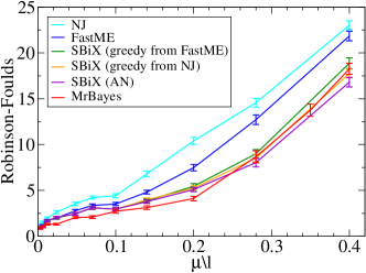
Figure 6: Performances comparison as a function of the per-site mutations rate. The evolutionary model used to generate phylogenies is the Kimura two parameters model with transition rate $\alpha=0.4$ and transversion rate $2\beta=0.6$. Robinson-Foulds measure for the reconstructed trees as a function of the mutation rate per site. We compare the performances of our SBiX algorithm (with $k=5$) with those of the following ones: Neighbor-Joining (NJ), FastME, SBiX greedy from NJ, SBiX greedy from FastME, SBiX simulated annealing, and MrBayes. Results are averages over $100$ independent realizations for each reported mutation rate. The error bars are standard errors. All the trees generated have $N=60$ leaves, and the sequence $l=1000$.

IV Discussion and conclusions

In this paper we have introduced a new algorithmic scheme for phylogeny reconstruction. Belonging to the family of Stochastic Local Search algorithms, our scheme crucially exploits two known properties of additive distance matrices, the four-points condition and the so-called Pauplin’s length. We proposed in particular a stochastic scheme where the correct topology is inferred through a series of swapping of the tree topology. When tested on artificially generated phylogenies our algorithmic scheme significantly outperforms state-of-art distance-based algorithms in cases of deviation from additivity due to high rate of back mutations. A significant improvement is also observed with respect to the state-of-art algorithms in case of high rate of horizontal transfer.

Such good performances are due to the way we differentially weight the different quartets contributions with a term inversely proportional to their length, and thus to their probability to be affected by back mutations. On the other hand further work is needed for a complete theoretical understanding of the algorithm. In particular, despite many attempts, we are, at present, unable to formulate the update strategy in terms of a state functional. Beside the interest in itself, this would open the way to analytic treatments as well as to algorithmic optimization strategies possibly more efficient than the Stochastic Local Search one.

As for the comparison of our algorithmic scheme with state-of-the art algorithms it is fair to observe that SBiX features a definitely larger computational complexity but, in practice, it is fast enough for reconstructing phylogenies up to a few thousands of leaves.

Though SBiX outperforms all competitors also in presence of horizontal transfers, the method is especially suited for dealing with non-additivity originated by double mutations. The issue of horizontal transfer is however central in many fields Doolittle et al. (2008), and we believe that formulating effective strategies to dealing with it, considering both phylogenetic trees and networks, is an open challenge for the next generation reconstruction algorithms and will be the aim of further studies.

It is worth mentioning how the applicability of phylogenetic algorithms has recently widened its scope. Many different fields have arisen in the last few years where a correct reconstruction of phylogenetic trees may reveal underlying relevant dynamical processes. For instance phylodynamics is a new field at the crossroad of immunodynamics, epidemiology and evolutionary biology, that explores the diversity of epidemiological and phylogenetic patterns observed in RNA viruses of vertebrates Grenfell et al. (2004); phylogeography is the study of the historical processes that may be responsible for the contemporary geographic distributions of individuals as well as of languages or viruses Avise (2000). In all these cases a strong effort is being devoted to the collection of comprehensive datasets and efficient and reliable algorithms are needed especially when deviations from perfect phylogenies become relevant.

V Appendix I

V.1 The equivalence with the Pauplin length minimization

We show here that our SBiX algorithm minimizes the Pauplin’s length when $k=0$ in the Eq. 2. In order to see this, we explicitly calculate the cost difference between, say, the configurations $((A,B),(C,D))$ and $((A,C),(B,D))$. We note that the sum on the considered quartets can be divided in three parts, in which one of the three distances $D_{1}$, $D_{2}$ and $D_{3}$ is respectively minimal (where, as already defined in the text, $D_{1}=d(a,b)+d(c,d)$, $D_{2}=d(a,c)+d(b,d)$ and $D_{3}=d(a,d)+d(b,c)$). After a little algebra one gets:

$$\Delta E=\sum\left(D_{2}-D_{1}\right)2^{-t(a,\alpha)-t(b,\beta)-t(c,\gamma)-t(d,\delta)},$$ (8)

where the sum is again over the $a\in A,b\in B,c\in C,d\in D$ and $\Delta E\equiv E_{((A,C),(B,D))}-E_{((A,B),(C,D))}$. Making use of the relation:

$$\sum_{i}2^{-t(i,r)}=1,$$ (9)

and of the equivalences: $2^{-t(a,b)}=2^{-t(a,\alpha)-t(b,\beta)}/2$ in the configuration $((A,B),(C,D))$ and $2^{-t(a,b)}=2^{-t(a,\alpha)-t(b,\beta)}/4$ in the configuration $((A,C),(B,D))$ (and the analogous relations for the other pairs of taxa), it is easy to prove that it holds:

$$\Delta E=4\Delta L_{P},$$ (10)

where $L_{P}$ is the Pauplin’s length and $\Delta L_{P}\equiv L_{P,((A,C),(B,D))}-L_{P,((A,B),(C,D))}$ is the difference of the Pauplin’s length between the two configurations.

V.2 Locality of the SBiX configuration cost

We give here an argument to prove that differences in the local cost of our SBiX method cannot be written as differences of a functional on the whole tree. If this was the case, a functional could be defined as $F(x)=F(x_{0})+\sum\Delta E_{i}$, where $F(x_{0})$ is the value taken by the functional in a reference configuration $x_{0}$, and $\Delta E_{i}$ are the cost differences along a path from $x_{0}$ to $x$. Moving in the space of tree’s topologies, we should obtain the same value of $F$ each time we visit the same topology, i.e., the difference of cost between two states does not depend on the path. This is not the case, as we explicitly checked, when the cost is defined as in Eq. 3 and $k\neq 0$.

VI Appendix II

VI.1 Discussion on the horizontal gene transfer modeling

In order to assure that the procedure of keeping the length of the horizontal transfer fixed to $l/4$, as for the results shown in the main text, does not alter the qualitative behaviour of the compared performances, we here show results where this restriction is relaxed. The Figure 7 is the analogous of Figure 5 (a) in the main text, with the difference that here the proportion of horizontal gene transfer is allowed to randomly vary in the interval [0,1/4].

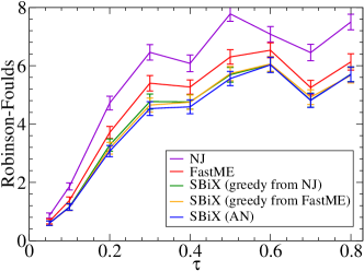
Figure 7: Performances comparison as a function of the horizontal transfer rate. Robinson-Foulds measure for the reconstructed trees as a function of the horizontal transfer rate of the generative model. We compare the performances of our SBiX algorithm (with $k=5$) with those of the following ones: Neighbor-Joining (NJ), FastME, the Pauplin length minimization algorithm (PAUPLIN) and the Normalized-Quartet (NQ) algorithm. Results are averages over $100$ independent realizations for each reported horizontal transfer rate The error bars are standard errors. All the trees generated have $N=60$ leaves, the mutation rate per site is kept fixed to $\mu/l=0.003$ while the sequences have fixed length $l=10000$.

VI.2 Discussion on the algorithmic computational complexity

VI.2.1 Generalities

Given the encouraging performance of the SBiX compared to other distance based algorithm we have run a detailed comparison with character based methods such as MrBayes Huelsenbeck and Ronquist (2001). For all our comparison we used MrBayes v3.1.2 on a standard linux platform, Intel Core(TM)2 CPU $@$ $2.40GHz$ and a cache size of $4096KB$. In the simulation we kept the default setting of the program ( Nruns = 2, Datatype = DNA, Nucmodel = 4by4, Nst = 1, Covarion = No, # States = 4, Rates = Equal ) and we did not specify any details of the model generator. The only parameters we tuned were: (i) the number Ngen of tree generated by the Monte Carlo Markov Chain (MCMC), (ii) the number Burnin of tree configurations discarded in the analysis. Parameter fixing depends critically on data, and in particular, the more the generative model departs from additivity, the longer the MCMC must be run in order to achieve convergence and obtaining a fair sampling of the likelihood landscape of the problem. A useful proxy for MCMC convergence is the average standard deviation of the partition split frequencies in the Nrun (in our case Nrun=2) MCMCs. One expects that this quantity, after a transient, approaches to zero for a sufficiently long number of iterations, reflecting the fact that the two Markov Chains become increasingly similar, sampling the same subspace of the problem.

VI.2.2 Computational complexity

Assessing precisely the computational complexity of MrBayes goes definitely beyond the scope of our work. We performed however a detailed analysis on a particular case for giving a fair comparison of the computational cost of the two strategies.

As a benchmark we used the two parameters Kimura generator (with transition rate $\alpha=0.4$ and transversion rate $2\beta=0.6$) discussed in the paper. We generated 100 realization of phylogenies, with sequence length $l=1000$, with a per-site mutation rate $\mu/l=0.1$, at different values of the number of leaves ranging from $N=15$ to $N=480$.

As a lower bound on the computational cost of MrBayes we decided to stop the simulation as soon as the average standard deviation of the partition split frequencies became lower than $0.05$. We intend this as a lower bound on the true computational cost since this can be considered as a good estimation only of the length of the transient regime. To ensure a fair equilibrium sampling one should check that the 2 Markov Chains maintains split values lower than our threshold for a number of generations large enough. For each of our samples we recorded the running time in seconds and we averaged over the 100 sample realizations.

$N$	$\overline{t}_{\mathrm{mb}}$	var$(t)_{\mathrm{mb}}$	samples (mb)	$\overline{t}_{\mathrm{SBiX}}$	var$(t)_{\mathrm{SBiX}}$	samples (SBiX)	ratio $\overline{t}_{\mathrm{mb}}/\overline{t}_{\mathrm{SBiX}}$
15	11	1	50	NA	NA	NA	NA
30	60	3	50	0.004	0.04	100	$1.5\times 10^{4}$
60	297	28	50	0.04	0.01	100	$7.4\times 10^{3}$
120	2277	258	50	0.64	0.02	100	$3.5\times 10^{3}$
240	17106	692	10	10.72	0.03	100	$1.5\times 10^{3}$
480	NA	NA	NA	200.67	0.03	100	NA
960	NA	NA	NA	5096.7	0.3	100	NA

Table 1: In this table we display the number of leaves $N$, the average running time in seconds $\overline{t}$, its variance, and the number of samples, both for MrBayes and SBiX algorithms. The last column reports the ratio between the average running times of MrBayes and SBiX.

On the same dataset we run the greedy version of SBiX starting from the configuration predicted by Neighbor Joining, and recorded the running time in seconds. In Table 1 we displays the comparison of the two algorithms. We did not display results for SBiX at $N=15$, the execution time being so tiny (order of milliseconds) that the measure would be strongly unreliable and basically dominated by input-output operating system tasks. We also do not present results for MrBayes at $N=480$, since each run would require a time larger than 32 hours.

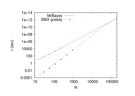
Figure 8: Plot of the average time of computation per sample (in seconds) as a function of the number of leaves of the phylogeny. All points represent an average over the respective number of samples as indicated in Table 1

In Figure 8 we plot the average running time per sample as a function of $N$ for both algorithm. We fitted MrBayes result with a simple power-law $a+bx^{c}$ obtaining as best fit $a=4(1)$ , $b=0.003(1)$, $c=2.8(1)$. The SBiX curve can be fitted with a simple fourth power behavior $Ax^{4}$, and the best fit value is $A=5.4(4)\cdot 10^{-9}$. Such a small prefactor allows SBiX to be faster than MrBayes to $N\sim 10^{5}$, despite the larger exponent (4 vs. 2.9) . Note that: (i) the running times at the crossing point are of the order of the thousand of years, and (ii) hardly a $10^{5}$ leaves genealogy could be of any interest.

VI.2.3 Computational cost as a function of the mutation rate

In the previous section we outlined the analysis of the computational complexity as a function of the number of taxa in the genealogy. In the paper we presented the accuracy of the different algorithms fixing the number of taxa ($N=60$) and varying the mutation rate per site $\mu/l$. While the running time of other algorithms (NJ, FastME, SBiX greedy) do not depend on the mutation rate, the running time required by MrBayes depends critically on it. In order to obtain a fair sampling of the space of trees we have run a number of preliminary simulations in order to have a quantitative estimate of the convergence time of the algorithm (the so-called burn-in time). Then we considered a measuring time either $50000$ or $100000$ Monte Carlo steps depending on the mutation rate (and on the burn-in time). In Table 2 we display the burn-in and measure times for the different values of the mutation rate. For each of the point we analyzed 100 different samples. The convergence time in the high mutation rate regime ($\mu/l>=0.2$) might be still too small, and for some of the samples the MCMC might not have reached convergence. In order to guarantee convergence for all samples one should double the burn-in time, requiring a time too long for our computational resources.

$\mu/l$	burn-in	measure	sec.
0.003	50000	50000	1300
0.006	50000	50000	1300
0.012	50000	50000	1300
0.024	50000	50000	1300
0.048	50000	50000	1300
0.070	50000	50000	1300
0.100	100000	100000	2600
0.140	100000	100000	2600
0.200	300000	100000	5200
0.280	300000	100000	5200
0.350	500000	100000	7800
0.400	700000	100000	12400

Table 2: In this table we display, for the different value of the per-site mutation rate $\mu/l$, the burn-in and the measure time in elementary Monte Carlo steps unit, together with an average estimate of running time in seconds.

VII Acknowledgments

The authors wish to thank Simone Pompei, Francesca Colaiori, Ciro Cattuto and Damián H. Zanette for many interesting discussions and suggestions. This research has been partly supported by the TAGora and ATACD projects funded by the European Commission under the contracts IST-34721 and 043415.

References

- Atteson (1997) Atteson, K. 1997. The performance of neighbor-joining algorithms of phylogeny reconstruction. In COCOON, 101–110.
- Avise (2000) Avise, J. C. 2000. Phylogeography: The History and Formation of Species. Harvard University Press.
- Bordewich et al. (2009) Bordewich, Magnus and Gascuel, Olivier and Huber, Katharina T. and Moulton, Vincent 2009. Consistency of Topological Moves Based on the Balanced Minimum Evolution Principle of Phylogenetic Inference. IEEE/ACM Trans. Comput. Biol. Bioinformatics 6(1):110–117.
- Cavalli-Sforza and Edwards (1967) Cavalli-Sforza, L. L. and A. W. F. Edwards. 1967. Phylogenetic analysis: Models and estimation procedures. American Journal of Human Genetics 19:233–257.
- Desper and Gascuel (2002) Desper, R. and O. Gascuel. 2002. Fast and accurate phylogeny reconstruction algorithms based on the minimum-evolution principle. Journal of Computational Biology 9:687–705.
- Doolittle et al. (2008) Doolittle, W. F., Nesbo, C.L., Bapteste, E. and Zhaxybayeva, O. 2008. Lateral gene transfer. Evolutionary Genomics and Proteonomics, M. Pagel and A. Pomiankowski (eds.) Sinauer:45-79.
- Erdös et al. (1998) Erdös, P. L., K. Rice, L. A. Szekely, T. J. Warnow, M. Steel and Y. J. Warnow. 1998. The short quartet method. In International Congress on Automata, Languages and Programming.
- Felsenstein (2004) Felsenstein, J. 2004. Inferring Phylogenies. Sinauer Assoc. Inc.
- Fitch and Margoliash (1967) Fitch, W. M. and E. Margoliash. 1967. Construction of phylogenetic trees. Science 155:279–284.
- Gascuel and Steel (2006) Gascuel, O. and M. Steel. 2006. Neighbor-Joining Revealed. Mol Biol Evol 23:1997–2000.
- Gascuel ed. (2007) Gascuel, O. (ed.) 2007. Mathematics of Evolution and Phylogeny. Oxford University Press.
- Gray and Atkinson (2003) Gray, R. D. and Q. D. Atkinson. 2003. Language-tree Divergence Times Support the Anatolian Theory of Indo-European Origin. Nature 426:435–439.
- Grenfell et al. (2004) Grenfell, B. T., O. G. Pybus, J. R. Gog, J. L. N. Wood, J. M. Daly, J. A. Mumford and E. C. Holmes. 2004. Unifying the epidemiological and evolutionary dynamics of pathogens. Science 303:327–332.
- Gusfield (1997) Gusfield, D. 1997. Algorithms on strings, trees, and sequences: computer science and computational biology. Cambridge University Press, New York, NY, USA.
- Hoos and Stützle (2005) Hoos, H. H. and T. Stützle. 2005. Stochastic Local Search: Foundations and Application. Morgan Kaufmann.
- Huelsenbeck and Ronquist (2001) Huelsenbeck, JP, Ronquist, F. 2001 MRBAYES: Bayesian inference of phylogenetic trees. Bioinformatics 17(8):754–755.
- Kimura, M. (1980) Kimura, M. 1980. A simple model for estimating evolutionary rates of base substitutions through comparative studies of nucleotide sequences. Journal of Molecular Evolution 16:111–120.
- Kirkpatrick et al. (1983) Kirkpatrick, S., J. Gelatt, C. D. and M. P. Vecchi. 1983. Optimization by Simulated Annealing. Science 220:671–680.
- Lazer et al. (2009) Lazer, D. et al. 2009. Social science: Computational social science. Science 323:721–723.
- Liu et al. (2009) Liu, K., S. Raghavan, S. Nelesen, C. R. Linder and T. Warnow. 2009. Rapid and accurate large-scale coestimation of sequence alignments and phylogenetic trees. Science 324:1561–1564.
- Mihaescu et al. (2007) Mihaescu, R., D. Levy and L. Pachter. 2007. Why neighbor-joining works. Algorithmica 54:1–24.
- Pagel (2009) Pagel, M. 2009. Human language as a culturally transmitted replicator. Nature Reviews Genetics 10:405–415.
- Pauplin (2000) Pauplin, Y. 2000. Diresct calculation of a tree length using a distance matrix. Journal of Molecular Evolution 51:41–47.
- Pybus and Rambaut (2009) Pybus, O. G. and A. Rambaut. 2009. Evolutionary analysis of the dynamics of viral infectious disease. Nature Reviews Genetics 10:540–550.
- Ragoussis (2009) Ragoussis, J. 2009. Genotyping technologies for genetic research. Annual Review of Genomics and Human Genetics 10:117–133.
- Renfrew et al. (2000) Renfrew, C., A. McMahon and L. Trask. 2000. Time Depth in Historical Linguistics. The McDonald Institute for Archeological Research.
- Robinson and Foulds (1981) Robinson, D. and L. Foulds. 1981. Comparison of phylogenetic trees. Mathematical Biosciences 53:131–147.
- Saitou and Nei (1987) Saitou, N. and M. Nei. 1987. The neighbor-joining method: a new method for reconstructing phylogenetic trees. Mol Biol Evol 4:406–425.
- Simonson et al. (2005) Simonson, A. B., J. A. Servin, R. G. Skophammer, C. W. Herbold, M. C. Rivera and J. A. Lake. 2005. Decoding the genomic tree of life. Proceedings of the National Academy of Sciences of the United States of America 102:6608–6613.
- Snir et al. (2008) Snir, S., T. Warnow and S. Rao. 2008. Short quartet puzzling: A new quartet-based phylogeny reconstruction algorithm. Journal of Computational Biology 15:91–103.