The Spitzer View of Low-Metallicity Star Formation: III. Fine Structure Lines, Aromatic Features, and Molecules

Abstract

We present low- and high-resolution Spitzer/IRS spectra, supplemented by IRAC and MIPS measurements, of 22 blue compact dwarf (BCD) galaxies. The BCD sample spans a wide range in oxygen abundance [12$+$log(O/H) between 7.4 and 8.3], and hardness of the interstellar radiation field (ISRF). The IRS spectra provide us with a rich set of diagnostics to probe the physics of star and dust formation in very low-metallicity environments. We find that metal-poor BCDs have harder ionizing radiation than metal-rich galaxies: [O iv] emission is $\;\buildrel>\over{\sim}\;$ 4 times as common as [Fe ii] emission. They also have a more intense ISRF, as indicated by the 71 to 160 µm luminosity ratio. Two-thirds of the sample (15 BCDs) show PAH features, although the fraction of PAH emission normalized to the total infrared (IR) luminosity is considerably smaller in metal-poor BCDs ($\sim$0.5% ) than in metal-rich star-forming galaxies ($\sim$10%). We find several lines of evidence for a deficit of small PAH carriers at low metallicity, and attribute this to destruction by a hard, intense ISRF, only indirectly linked to metal abundance. Our IRS spectra reveal a variety of H₂ rotational lines, and more than a third of the objects in our sample (8 BCDs) have $\lower 2.15277pt\hbox{$\;\buildrel>\over{\sim}\;$}3\sigma$ detections in one or more of the four lowest-order transitions. The warm gas masses in the BCDs range from $10^{3}$ to $10^{8}$ $M_{\odot}$, and can be comparable to the neutral hydrogen gas mass; relative to their total IR luminosities, some BCDs contain more H₂ than SINGS galaxies.

Facilities: Spitzer ()

1 Introduction

First IRAS and ISO, then SCUBA and COBE, and most recently Spitzer have convincingly shown that most of the star formation in the universe is enshrouded in dust. Large populations of infrared-luminous galaxies at $z\lower 2.15277pt\hbox{$\;\buildrel<\over{\sim}\;$}$1.5 contribute to about 70-80% of the far-infrared and 30% of the sub-millimeter backgrounds, and are probably responsible for most of the star-formation activity at high redshift (e.g., Chary & Elbaz, 2001; Le Floc’h et al., 2005; Dole et al., 2006). Indeed, half the energy and most of the photons in the universe come from the infrared spectral region (e.g., Hauser & Dwek, 2001; Franceschini et al., 2008).

That dust is so prominent in the high-redshift universe may appear surprising, since it has been assumed that dust would be absent in low-metallicity environments. However, recent theoretical developments challenge the assumption that dust is absent in metal-poor gas. Large amounts of dust can be created on short timescales by supernovae (SNe) and Asymptotic Giant Branch stars which evolve in a metal-free ISM (e.g., Todini & Ferrara, 2001; Schneider et al., 2004; Nozawa et al., 2007; Bianchi & Schneider, 2007; Valiante et al., 2009). Observationally, the copious dust emission observed at very high redshifts ($z\lower 2.15277pt\hbox{$\;\buildrel>\over{\sim}\;$}6$) in quasars implies that indeed dust can form rapidly at early epochs (Bertoldi et al., 2003). Although luminous quasars can hardly be considered as typical examples of star-forming environments, observations of sub-millimeter galaxies (SMGs, Chapman et al., 2005) and dust-obscured galaxy populations (DOGs, Dey et al., 2008) also suggest that early star formation episodes can also be very intense and relatively brief. However, exactly how these massive starbursts occur and evolve is not yet clear. The short interval in which star formation and the ensuing chemical enrichment and dust formation convert a dust-free metal-free environment to a dusty metal-rich one by redshift $\sim$6 is as yet unobserved, and studies of such transitions remain a major observational challenge.

The Local Universe is home to star-forming dwarf galaxies that are of much lower metallicity than those observed thus far at high redshift. Over the last thirty years or so, only a handful of blue compact dwarf (BCD) galaxies have been discovered with 12$+$log(O/H)$\sim$7.2. Despite intensive searches, only one BCD, SBS 0335$-$052 W, is known to host Hii regions with 12$+$log(O/H)$\leq$7.1 (Izotov et al., 2009). Even at these extremely low metallicities, BCD spectral energy distributions (SEDs) can be dominated by infrared dust reprocessing of ultraviolet radiation from young massive stars (e.g., SBS 0335$-$052 E and I Zw 18: Thuan, Sauvage, & Madden, 1999; Houck et al., 2004b; Wu et al., 2007). Because such galaxies are chemically unevolved, they can provide a window on primordial galaxy formation and evolution. This is, in some sense, a “local” approach to a cosmological problem. If we can study the properties of a metal-poor ISM and its constituents locally, we may be able to better understand the high-redshift transition from metal-free Population III (Pop III) stars to the chemically evolved massive galaxies typical of the current epoch.

We adopt here this “local” approach. With the aim of characterizing the properties of star and dust formation in a metal-poor ISM, we have used the Spitzer Space Telescope to study a sample of nearby low-metallicity star-forming dwarf galaxies. This is the third in a series of papers; the first two papers have focused on two particular BCDs, Haro 3, the highest metallicity object in our sample (Hunt et al., 2006), and Mrk 996, a BCD with an unusually dense and compact nuclear Hii region (Thuan et al., 2008). Here, we present for the first time the entire sample of 23 BCDs, and report on its spectral properties, as derived from IRS observations. The sample has been carefully chosen to span a wide range in oxygen abundance: 12$+$log(O/H) varies between 7.4 and 8.3, with a median of 7.9. About a quarter of the objects in the sample are in the eXtremely Metal-Deficient (XMD) or Extremely Metal-Poor Galaxy (EMPG) range (12$+$log(O/H)$\;\buildrel<\over{\sim}\;$7.65 Pustilnik & Martin, 2007; Brown et al., 2008). Thus our sample comprises the largest number of XMDs/EMPGs to date with good signal-to-noise IRS spectra.

In $\S$2, we describe the sample selection criteria, together with the Spitzer observations and the data reduction methods. In $\S$3, we derive fluxes of lines and features in the spectra by fitting them with PAHFIT (Smith et al., 2007). We present and discuss our results for the infrared (IR) fine-structure (FS) lines in $\S$4, the aromatic features in $\S$5, and in $\S$6, the molecular lines. Our conclusions are summarized in $\S$7.

2 Sample Definition, Observations, and Data Reduction

One of the most important factors in shaping the SED at low metallicity is the hardness and intensity of the interstellar radiation field (ISRF). The ISRF hardness and intensity govern dust properties such as the grain size distribution and temperature. Hard and intense ISRFs may destroy small grains all together, thus suppressing the aromatic or polycyclic aromatic hydrocarbon features (PAHs) which are typical of metal-rich starburst galaxies (e.g., Voit, 1992; Madden et al., 2006; Smith et al., 2007). In the post-ISO and post-Spitzer eras, ratios of IR lines of neon have often been used to quantify the hardness of the ISRF in star-forming galaxies (e.g., Thornley et al., 2000; Dale et al., 2006). However, since we have selected the objects in our sample on the basis of their optical spectra, we have quantified ISRF hardness optically, with the ratio of the nebular Heii $\lambda$ 4686 emission line relative to H$\beta$. The Heii line, with an ionization potential of 54.4 eV, is a good indicator of a hard ultraviolet (UV) radiation field. Nebular Heii lines are predicted to be very strong in metal-free (or nearly metal- free) primordial galaxies (Schaerer, 2002, 2003), although no Heii-emitting high-redshift galaxy (z$\;\buildrel>\over{\sim}\;$5) has yet been discovered (e.g., Nagao et al., 2008).

However, some low-redshift low-metallicity BCDs are known to show strong nebular Heii $\lambda$4686 emission with Heii/H$\beta$$\;\buildrel>\over{\sim}\;$3% (Guseva, Izotov & Thuan, 2000; Izotov & Thuan, 2004; Thuan & Izotov, 2005). We have selected 23 objects so that they span a wide range in Heii/H$\beta$. Roughly 1/3 of the sample consists of objects having strong Heii emission, with Heii/H$\beta$$\;\buildrel>\over{\sim}\;$2%; another third have intermediate Heii emission with Heii/H$\beta$$\sim$1-2%, and the remaining third has weak or no Heii emission, with Heii/H$\beta$$\;\buildrel<\over{\sim}\;$1%. This wide range of Heii strength in our sample also provides a large range in metallicity as there is a loose correlation between the two quantities (Thuan & Izotov, 2005). The general properties of the sample are given in Table 1.

The observations presented in this paper are part of our GO Spitzer program (PID 3139) for 23 BCDs. In the course of this program, we have obtained IRS spectra in the low- and high-resolution modules (SL, SH, LH Houck et al., 2004a), IRAC images at 4.5 and 8 µm (Fazio et al., 2004), and MIPS images at 24, 71, and 160 µm (Rieke et al., 2004). For all instruments, the data reduction starts with the Basic Calibrated Data (bcd). The corresponding masks (the DCE masks), furnished by the Spitzer Science Center pipeline, were then used to flag potential spurious features in the images, such as strong radiation hits, saturated pixels, or nonexistent/corrupted data.

2.1 IRS spectroscopy

Spectroscopy was performed in the staring mode, in both orders of the Short Low-resolution module (SL1, SL2) and with the Short and Long High-resolution modules (SH, LH) (Houck et al., 2004a). Thus, we have obtained low-resolution spectra from 5.2 to 14.5 µm (R$\simeq$64-128), and high-resolution spectra from 9.6 to 37.2 µm (R$\simeq$600). We have used different acquisition schemes, depending on the brightness of the source as measured by its scaled H$\beta$ flux. Sources were centered in the slits by peaking up on 2MASS stars.

The individual bcd frames were processed by the S13.2.0 version of the SSC pipeline, which performs ramp fitting, dark current subtraction, droop and linearity corrections, flat-fielding, and wavelength and flux calibrations. Because the pipeline does not include background subtraction, we have constructed, for the low-resolution long-slit spectra, a coadded background frame from the bcd observations with the source in the opposing nod and off-order positions (see also Weedman et al., 2006). Coadding was performed with the sigma-clipping option of the imcombine task in IRAF. The inclusion of off-order and off-nod frames in the background image means that the total integration time on the background is three times that on the source, thus improving the signal-to-noise of the two-dimensional (2D) subtraction.

We did not acquire a separate background spectrum for the high-resolution SH and LH spectra, and the slit size precludes using the same procedure as for the SL module. Therefore we subtracted the background from the SH and LH observations using the one-dimensional (1D) spectra as described below. The SH and LH 2D bcd images were coadded in the same way as for the SL modules, and corrections for sporadic bad pixels and cosmic ray hits were carried out manually by inspection of the images at the separate nod positions.

We extracted the source spectra with SPICE, the post-pipeline IRS package furnished by the SSC. Before extraction, all spectra at separated nod positions were cleaned with the IRSCLEAN algorithm (http://ssc.spitzer.caltech.edu/postbcd/irsclean.html). The automatic point-source extraction window was used for all modules. Automatic extraction uses a variable-width extraction window which scales with wavelength in order to recover a constant fraction of the diffraction-limited instrument response. For the SL spectra, this gives a 4-pixel (7$\farcs$2) length at 6 µm, and an 8-pixel length (14$\farcs$4) at 12 µm; the slit width is 3$\farcs$6 for both SL modules. At high resolution, the SPICE extraction was performed over the entire slit (4$\farcs$7$\times$11$\farcs$3 SH; 11$\farcs$1$\times$22$\farcs$3 LH). Orders were spliced together by averaging, ignoring the noisy regions at the red end of each order (e.g., Armus et al., 2004). Then the individual spectra were box-car smoothed to a resolution element, and clipped in order to eliminate any remaining spikes in the high-resolution data. Finally, the two spectra for each module (one for each nod position) were averaged.

Background was subtracted from the 1D SH spectra by defining a level from the overlap region with the SL spectra, from which we had subtracted a 2D background. Specifically, the difference between the 2D background-subtracted SL and SH spectra was minimized over the substantial region where they overlap in wavelength ($\sim$5 µm). The spectral shape of the background was given by the model of Reach and coworkers, and the multiplicative constant by the minimization process. Subsequently, the LH background was subtracted in an analogous way, by minimizing the difference between the SH and LH spectra over their overlap region ($\lesssim$1 µm).

This “bootstrapping” procedure for background subtraction in the high-resolution modules should in principle eliminate the need for scaling adjustments. However, its accuracy depends on the unresolved nature of the sources in the spectral apertures. We measured the source sizes by fitting Gaussians to the IRAC 7.9 µm and MIPS 24 µm images. The mean (and median) image FWHM is 3$\farcs$7 at 7.9 µm, and 6$\farcs$2 at 24 µm. The SL1 slit width is 3$\farcs$6, so most of the sources are sufficiently compact to not significantly exceed the SL1 slit size. The resolution of MIPS24 is $\sim$6″, making the BCDs essentially unresolved at these longer wavelengths; in fact, the characteristic diffraction pattern is seen in all the MIPS24 images. The FWHM of the largest source at 24 µm (Tol 1924$-$416) is 10″, so even in the most extreme case, the LH slit width of 11$\farcs$1 completely encompasses the BCD light at 24 µm. Our assumption of point-like morphologies at Spitzer wavelengths thus appeared to be reasonably justified. Nevertheless, for a few (of the largest) sources, the level of the background needed to be adjusted slightly to provide a smooth transition among the modules. In any case, the 24 µm flux as measured from MIPS is generally consistent with the continuum level derived for the IRS spectra (see below).

We have obtained IRAC and MIPS photometry for all 23 BCDs in our sample. However, we have IRS observations for only 22 BCDs. One BCD, SBS 0940$+$544, has an IRS observation in the Guaranteed Time program (PID 85). Thus, we present here IRS results for only 22 objects, and will incorporate SBS 0940$+$544 into our sample in a future paper.

2.2 IRAC and MIPS Imaging

Although the focus of this paper is on the IRS spectra of our sample objects, we briefly describe their Spitzer photometric data because we need photometric quantities such as the total IR luminosity ($L_{\rm TIR}$) to properly interpret their spectral properties. A more detailed description of the photometry and reduction procedures can be found in Hunt et al. (2006, Haro 3) and Thuan et al. (2008, Mrk 996). The discussion of the photometric data of the whole sample is deferred to a future paper on SEDs.

Briefly, we acquired IRAC images in two filters, 4.5 and 7.9 µm, each with two sets of four frames in the high dynamic range mode. The individual bcd frames were processed with the S14.0.0 version of the SSC pipeline (see the IRAC Data Handbook). The bcd frames (corrected for “banding” effects for bright sources) were coadded using MOPEX, the image mosaicing and source-extraction package provided by the SSC (Makovoz & Marleau, 2005). Pixels flagged by the masks were subsequently ignored. Additional inconsistent pixel values were removed by means of the MOPEX outlier rejection algorithms, in particular the dual-outlier technique, together with the multiframe algorithm. The frames were corrected for geometrical distortion and projected onto a “fiducial” (refined) coordinate system with pixel sizes of 1$\farcs$20, roughly equivalent to the original pixels. Standard linear interpolation was used for the mosaics. The noise levels in our post-pipeline MOPEX IRAC mosaics are comparable to or lower than those in the SSC products.

Our MIPS images were acquired in the Fixed Cluster-Offset mode in all three channels, with offsets of 12″ in two additional pointings. The individual bcd frames were processed by the the S14.4.0 version of the SSC pipeline, which converts the integration ramps inherent to the MIPS detectors into slopes, and corrects for temporal variations of the slope images (Gordon et al., 2005). As for the IRAC images, we processed the dithered bcd frames in the spatial domain with MOPEX. The DCE masks and the static masks were used to flag pixels which were subsequently ignored. The MOPEX outlier rejection was used to remove any additional spurious pixel values, with the dual-outlier and multiframe algorithm as for the IRAC frames. Geometrical distortion was corrected before projecting the frames onto a fiducial coordinate system with pixel sizes of 1$\farcs$20 for MIPS24, roughly half of the original pixel size of 2$\farcs$5. Pixel sizes of the final mosaics at 71 and 160 µm are also approximately half the originals, i.e. 4$\farcs$95 at 71µm and 8$\farcs$0 at 160 µm. Unlike the IRAC coadds, we incorporated the sigma-weighting algorithm because it gave less noisy MIPS mosaics than without. Standard linear interpolation was used in all cases. In all three channels, our MOPEX mosaics are superior to those provided by the automated post-pipeline reduction.

2.3 IRAC and MIPS Photometry

We have performed aperture photometry on the IRAC and MIPS images with the IRAF photometry package apphot, taking care to convert the MJy/sr surface brightness units of the images to integrated flux units. The background level was determined by averaging several adjacent empty sky regions. Fluxes were determined at radii where the growth curve has become asymptotically flat. In many cases, there are multiple sources within the IRS apertures, and we used subjective judgment to match photometry with the spectroscopic slit. Following Draine & Li (2007), these fluxes were used to derive the “color temperature” between 71 and 160 µm, $\langle\nu{\rm L}_{\nu}(71)\rangle/\langle\nu{\rm L}_{\nu}(160)\rangle$, and the total infrared flux (TIR):

$$L_{\rm TIR}\,=\,0.95\,\langle\nu L_{\nu}\rangle_{7.9}+1.15\,\langle\nu L_{\nu}\rangle_{24}+\langle\nu L_{\nu}\rangle_{71}+\langle\nu L_{\nu}\rangle_{160}$$

Both quantities will be pertinent for the discussion of the spectra.

In order to check our reduction and calibration procedures for both the IRS and MIPS, we have compared the MIPS 24 µm total fluxes with the continuum levels in the IRS spectra. Such a comparison (see below) shows good general agreement, implying that both the IRS flux calibration (in the case of a point-source) and background subtraction and the derivation of the total MIPS flux have been done correctly. The only exception is UM 311, which is in a crowded field (there are several point sources in close proximity to a spiral galaxy), and thus its photometry is probably contaminated by other sources.

All targets were detected at 24 and 71 µm. However, at 160 µm, we obtained only upper limits (ULs) for 6 of them. As a consequence of a Spitzer queue problem, SBS 1030$+$583 has no MIPS24 observations.

3 Spectral Analysis

The flux emitted by aromatic (or PAH) features constitutes a large fraction of the IR energy budget in a typical star-forming galaxy spectrum. However, these features are known to decrease in intensity or even disappear at low metallicities (Engelbracht et al., 2005; Madden et al., 2006; Wu et al., 2006; Engelbracht et al., 2008). Our sample contains many metal-deficient objects and is thus uniquely able to address the behavior of PAH emission at low metallicities. In order to directly compare the results for our low-metallicity sample with those for an existing well-defined set of more metal-rich galaxies, we wanted to analyze our IRS spectra in the same manner as this latter set. This consideration dictated the use of PAHFIT (Smith et al., 2007), an IDL procedure which was developed for and applied to the Spitzer Nearby Galaxy Survey (SINGS, Kennicutt et al., 2003).

PAHFIT is particularly suited for separating emission lines and PAH features (e.g., the PAH blend at 12.6–12.7 µm and the [Ne ii] line at 12.8 µm), as well as measuring faint PAH features superimposed on a strong continuum. Broad “plateaus” underlying the 8 µm and 16-17 µm emission (Peeters et al., 2002, 2004b) and strong silicate absorption at 9.7 µm can make the measurement of broad PAH bands exceedingly difficult in those wavelength regions. PAHFIT overcomes this problem by fitting simultaneously the spectral features, the underlying continuum, and the extinction, and gives quantitative estimates and uncertainties for all parameters. Drude profiles are fitted to the PAH features, and Gaussian profiles to the molecular hydrogen and fine-structure lines. In addition to PAHFITting the spectra, we also measured emission line fluxes over the entire IRS range by fitting Gaussian profiles. Our strategy for deriving quantitative measurements from the IRS spectra is described in the following.

3.1 PAHFIT

Our spectra have a higher resolution than those normally fitted with PAHFIT, specifically for wavelengths $\geq$14.5 µm where we have no low-resolution spectra. Hence, after binning the spectra to a 0.03 µm resolution, and fitting the entire spectrum, we use only the spectral lines measured with PAHFIT having $\lambda$ $\leq$ 14.5 µm. In contrast, we adopt all the dust features fitted by PAHFIT over the entire IRS range. We modified the PAHFIT IDL code to allow the central wavelengths and widths of the Drude profiles to vary, and experimented with different weighting schemes. We also tried several different combinations of dust continuum temperatures, but these did not influence the fit results. PAHFIT was run with three different options, including mixed extinction, screen extinction, and fixing extinction to zero.

The nominally best fits (those with lowest $\chi_{\nu}^{2}$) for 11 BCDs had non-zero extinction. However, in every case but Haro 3 and Mrk 996, the statistical significance of the fit was comparable to similar fits, but with zero extinction. Hence, when possible, we opted for the fit with no extinction [$\tau(9.7)$ = 0].

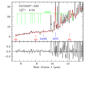
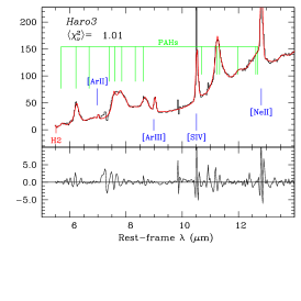
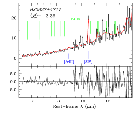
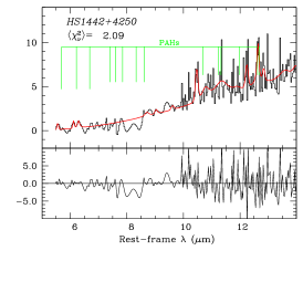
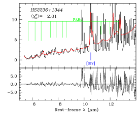
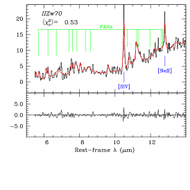
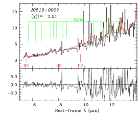
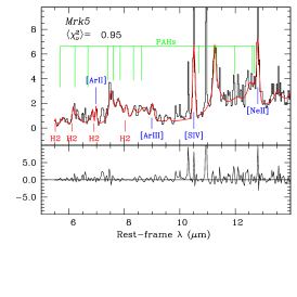
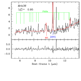
Figure 1: IRS SL$+$SH spectra from 1 to 15µm, with the best-fitting PAHFIT model superimposed shown as a red curve. The vertical axis is in units of mJy. Significant emission-line identifications are shown as labeled vertical lines. The top panels report the best-fit reduced $\chi^{2}_{\nu}$, obtained over the wavelength region shown. The bottom panels show the residuals from the PAHFIT models.

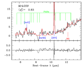
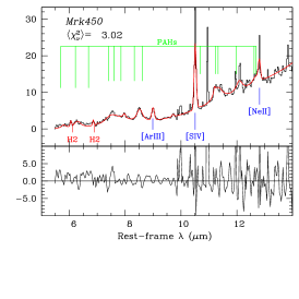
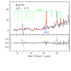
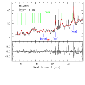
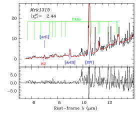
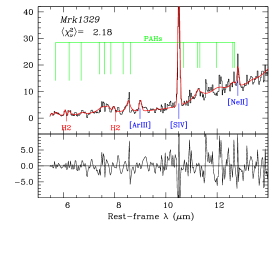
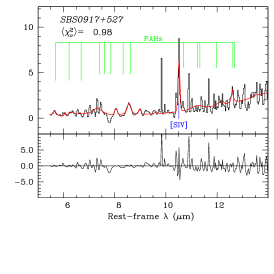
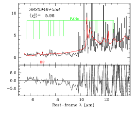
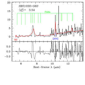
Figure 1:  continued.

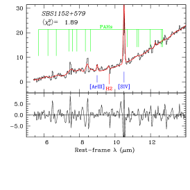
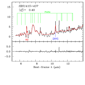
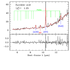
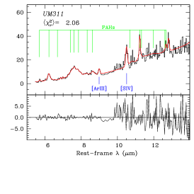
Figure 1:  continued.

The results are shown in Figure 1. The top panels show the best-fit PAHFIT model as a red curve, and the bottom panels give the residuals. The reduced $\chi_{\nu}^{2}$ given in each panel in the figures is calculated from the residuals of the fit up to 14.5 µm, normalized by the mean spectral uncertainty over the same spectral range. The figures show that the residuals are generally quite well-behaved, and that $\chi_{\nu}^{2}$ is generally sufficiently small to imply a good fit. Uncertainties on the integrated line fluxes were estimated in two ways. The standard deviation $\sigma$ per pixel of the continuum was measured individually in a relatively clean region of each SL, SH, and LH spectrum. A first estimate of the uncertainty in the line flux, assumed to be spread over 3 pixels, is taken to be $3\times 3\sigma$. This is compared with a second uncertainty estimate, the one given by PAHFIT for each spectral feature. The largest of the two estimates was then chosen to be the final uncertainty of the measurement. Table 2 reports all FS lines with $\lambda\leq$14.5 µm detected at the $\lower 2.15277pt\hbox{$\;\buildrel>\over{\sim}\;$}3\sigma$ level with PAHFIT, and Table 3 lists the dust features.

3.2 Gaussian Fitting of Emission Lines

We fitted all possible molecular and FS emission lines with Gaussian profiles, taking the integrated fitted flux as the measure of the total flux in the line. When necessary, we used multiple Gaussian profiles to deblend adjacent lines (e.g., [O iv] and [Fe ii] at $\sim$26 µm). Linear continua were fitted simultaneously, taking care to define the continuum regions well beyond the Gaussian wings.

In order for a spectral feature to be identified with a known emission line, its rest-frame wavelength shift from the laboratory wavelength had to to be $\leq$0.065 µm (for each object, we correct the observed spectrum to its rest frame by using the optical redshift listed in Table 1). Each emission line was measured several times, varying the continuum positions and blending parameters, to obtain an additional estimate of the uncertainty. The uncertainty on the integrated flux was then taken to be the larger of the two following estimates: the standard deviation of the ensemble of different measurements, or 9 times the standard deviation $\sigma$ of the continuum fluctuations, as described above (assuming the line is spread over 3 pixels). To guard against false detections from bad pixels or spectral glitches, we also required that the average of the two nod positions have a signal-to-noise $\geq$3. Table 4 reports the long-wavelength FS fluxes we obtain from these measurements.

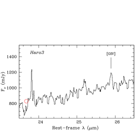
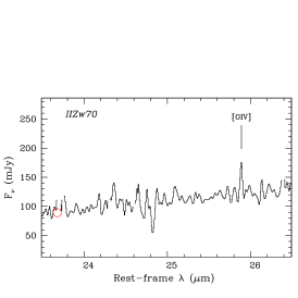
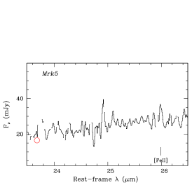
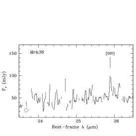
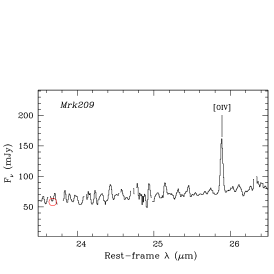
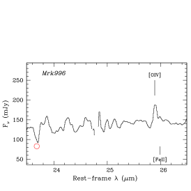
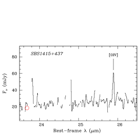
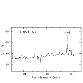
Figure 2: IRS LH spectra of the 26µm region around [O iv] and [Fe ii] for those objects with either [O iv] or [Fe ii] detections. As in Fig. 1, all marked features are considered significant (see Table 4). The MIPS24 total flux is marked with a red open circle. Only those spectral points with S/N$>$3 are shown.

For the objects where [O iv] or [Fe ii] was detected, blown-up parts of the spectra showing the 26µm region are given in Figure 2. Although we detect [O iv] at 3$\sigma$ (2$\sigma$) in 7 (9) galaxies, [Fe ii] is detected only in 2 (5 at 2$\sigma$). This result will be discussed in more detail in $\S$4.4. The extremely high-excitation lines [Nev] (ionization potential of 97.1 eV) at 14 and 24 µm are not detected in our data for any BCD. The MIPS 24 µm continuum level is also shown in Fig. 2 by an open circle. As stated in $\S$2.3, the IRS spectra and MIPS 24 µm total fluxes are consistent, except for UM 311 which is in a crowded field.

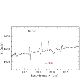
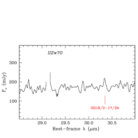
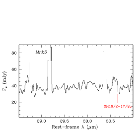
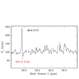
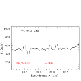
Figure 3: Close-up of tentative H₂O (29.8µm) and OH (28.9 µm) detections. All marked lines are considered to be significant detections (see Table 6). Only those spectral points with S/N$>$3 are shown.

In addition to the definite presence of H₂, a few spectra shown in Fig. 3 also tentatively suggest the presence of two other molecules, OH ($\sim$28.9, 30.3, 30.7 µm) and H₂O  ($\sim$29.8 and 29.9 µm). Table 5 gives the H₂ line fluxes (including those measured by PAHFIT for $\lambda\lesssim$ 14.5 µm, see above), and Table 6 reports the other molecules. These detections will be discussed further in $\S$6.

3.3 Comparison of Fitting Techniques

To judge the reliability of our line flux measurements, we have compared the fluxes of those emission lines that fall in the short-wavelength region of the spectra ($\lambda\leq$ 14.3 µm), and that have been measured in two different ways: first by PAHFIT and second by individual Gaussian fits. For strong lines with fluxes $\sim 2\times 10^{-17}$ W m^-2, the difference between these two methods is $\;\buildrel<\over{\sim}\;$4%; for faint lines with fluxes $\sim 5\times 10^{-18}$ W m^-2, the difference can be as large as 25%. The larger discrepancy for the fainter lines can be attributed to the choice of different continuum levels in the two methods. This is the main reason why we preferred to use PAHFIT for the short-wavelength region. However, the overall agreement between the two methods is sufficiently good to conclude that we can reliably compare short- and long-wavelength line fluxes, and that we do not introduce systematic differences in measuring them with slightly different methods.

Although PAHFIT corrects for dust extinction, we have not applied an analagous correction to the line fluxes for $\lambda\geq$14.5 µm. Such corrections would be applicable only to two sources, Haro 3 and Mrk 996. Haro 3, with $\tau(9.7)$ = 0.39, would have a correction $\;\buildrel<\over{\sim}\;$25% for wavelengths longer than 15 µm; Mrk 996 would have a 2% correction. Hence, because the correction for both objects are comparable to or smaller than uncertainties in the line fluxes, we did not apply them to the long-wavelength measurements.

4 The Ionized Component of the ISM

The spectral region covered by Spitzer/IRS provides a wealth of diagnostics to probe the physics of the ISM at low metallicity. The FS lines allow us to assess the physical conditions of the ISM, including the spectral shape or hardness of the ISRF and the density of the ionized gas. These quantities affect the dust properties by causing changes in the temperature of the “classical” grains, and by altering the stochastic emission from the aromatic features. They constrain the molecular content through dissociation and excitation processes.

4.1 The Hardness of the Interstellar Radiation Field

The IR FS lines span a wide range of ionization potentials and are thus sensitive diagnostics of the ionized ISM in BCD Hii regions. We focus first on diagnostics of the ISRF hardness. In their discussion, we will attempt to distinguish among the interdependent effects of ISRF hardness, ISRF intensity, and nebular metallicity.

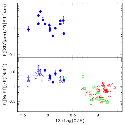
Figure 4: [S iv]/[S iii] (18.7 µm) flux ratios (top panel) and [Ne iii]/[Ne ii] ratios (bottom) plotted against the nebular oxygen abundance, 12$+$log(O/H). The BCDs in our sample are shown as filled circles, while the SINGS galaxies (Dale et al., 2009) as open squares (Hii region-nuclei) and open triangles (AGN). The horizontal dotted line in the lower panel shows the mean neon ratio (5.42) for 12$+$log(O/H)$\leq$8.3 (not considering lower limits).

Traditionally, flux ratios of high-ionization species have been used to measure the ISRF hardness, or equivalently the UV slope of its spectrum, which is sensitive to the effective temperatures of the ionizing stars. In the IR range, the [Ne iii]/[Ne ii] and [S iv]/[S iii] flux ratios are usually adopted (e.g., Thornley et al., 2000; Giveon et al., 2002). Such flux ratios also depend on the ionization parameter $U$, defined as $U\,=\,Q/4\pi R_{*}n_{\rm e}c$, where $Q$ is the number of ionizing photons, $n_{\rm e}$ is the electron density, and $R_{*}$ is the radius of the star-forming region (e.g., Thornley et al., 2000). We first examine whether these ratios depend on metallicity as shown in Fig. 4. The top panel shows that within our sample there may be a very slight dependence of the [S iv]/[S iii] ratio on metallicity, although with a very large scatter (there are no SINGS data for the variation of this flux ratio with abundance). The bottom panel shows that there is very little correlation of the [Ne iii]/[Ne ii] flux ratio with oxygen abundance within our sample alone. However, when the SINGS data are included, it is clear that the low-metallicity BCDs show considerably higher neon ratios than the more metal-rich SINGS galaxies (Dale et al., 2009). The SINGS galaxies span an abundance range of roughly a factor of 10, from 12$+$log(O/H) $\sim$8.4 to 9.4, and our sample fills in the decade below, down to 12$+$log(O/H) $\sim$7.5. Considering the two samples together, the bottom panel shows an increase of the [Ne iii]/[Ne ii] flux ratio by a factor of $\sim$10 from 12$+$log(O/H) $\sim$9.4 down to $\sim$8.2. Then the curve flattens out into a “plateau” for lower abundances, with [Ne iii]/[Ne ii] $\sim$5. Again, the scatter of the [Ne iii]/[Ne ii] flux ratio at a given oxygen abundance is large, indicating that metallicity cannot be the main parameter controlling the hardness of the ISRF. Similar behavior is shown also in previous metal-poor samples (Wu et al., 2006; Hao et al., 2009).

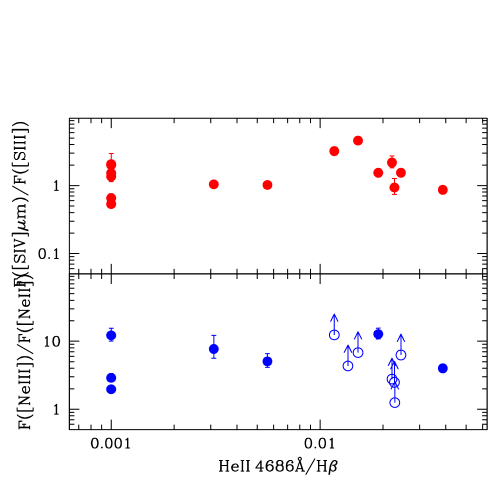
Figure 5: [S iv]/[S iii] (18.7 µm) flux ratios (top panel) and [Ne iii]/[Ne ii] ratios (bottom) plotted against the optical Heii/H$\beta$ ratio.

Our sample was defined on the basis of the optical Heii/H$\beta$ ratio which gives an independent estimate of the ISRF hardness. However, within our sample, there is no correlation between the [Ne iii]/[Ne ii] and [S iv]/[S iii] ratios and the Heii/H$\beta$ ratio as shown in Fig. 5. A possible reason for this lack of correlation is that the IR and optical ratios do not probe the same excitation energy. The ionization potentials for [Ne iii] and [Ne ii] are respectively 41.0 eV and 21.6 eV, while they are respectively 34.8 eV and 23.3 eV for [S iv] and [S iii]. These ionization potentials are well below that of He⁺ which is 54.4 eV. Thus, the ISRF UV energies probed by the neon and sulfur lines are too soft compared to those probed by the Heii ratio.

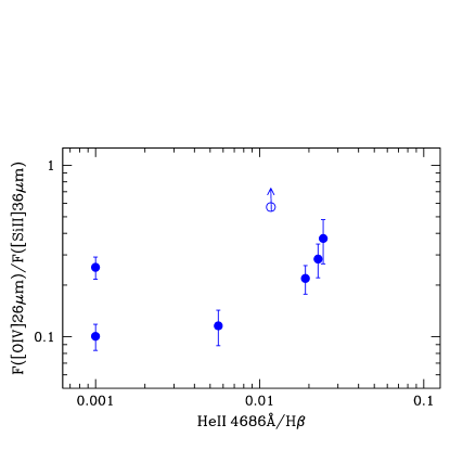
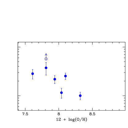
Figure 6: [O iv]/[Si ii] flux ratios plotted against the optical Heii/H$\beta$ ratio (left panel) and 12$+$log(O/H) (right). The figure shows only those objects with 3$\sigma$ detections or better in the [O iv] line.

We have therefore examined the relation between the [O iv]/[Si ii] and Heii/H$\beta$ ratios; the ionization potential of [O iv] is 54.9 eV, similar to that of He⁺ (54.4 eV), while that of [Si ii] is only 8.2 eV. Since both silicon and oxygen are products of core-collapse supernovae (SNe), the [O iv]/[Si ii] ratio should not be subject to abundance anomalies. The left panel of Fig. 6 shows a weak correlation between the two ratios for the BCDs in our sample: a high [O iv]/[Si ii] ratio is associated with a higher Heii/H$\beta$, at a confidence level of $\sim$93% (one-tailed). Higher [O iv]/[Si ii] is associated with lower nebular O/H abundance (right panel of Fig. 6), at a $\sim$98% confidence level (one-tailed). This last correlation is similar to the one between Heii/H$\beta$ and O/H (Thuan & Izotov, 2005). Evidently, lower metallicity galaxies tend to have generally harder ionizing radiation.

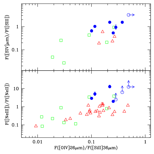
Figure 7: [Ne iii]/[Ne ii]/ and [S iv]/[S iii] (18.7 µm) plotted against the [O iv]/[Si ii] flux ratios. As in Fig. 4, BCDs are shown as filled circles, and the SINGS galaxies (Dale et al., 2009) as open squares (Hii region-nuclei) and open triangles (AGN). The figure shows only those objects with 3$\sigma$ detections or better in the [O iv] line.

Although the BCDs by themselves show little correlation between the [O iv]/[Si ii] ratio and the [Ne iii]/[Ne ii] and [S iv]/[S iii] ratios, when SINGS galaxies are included, there is a definite correlation. Fig. 7 illustrates this, and suggests that in star-forming galaxies the presence of hard radiation as probed by the [O iv]/[Si ii] ratio implies also the presence of less hard radiation as probed by the [Ne iii]/[Ne ii] and [S iv]/[S iii] ratios.

4.2 The Intensity of the Interstellar Radiation Field

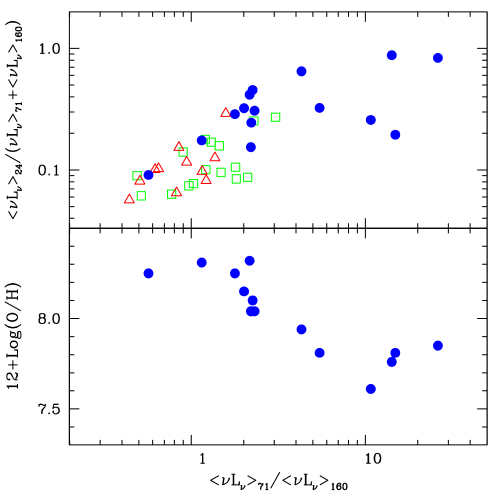
Figure 8: $\langle\nu{\rm L}_{\nu}\rangle$₂₄/($\langle\nu{\rm L}_{\nu}\rangle$${}_{71}+$ $\langle\nu{\rm L}_{\nu}\rangle$₁₆₀ (upper panel) and 12$+$log(O/H) (lower) plotted against the MIPS ratio $\langle\nu{\rm L}_{\nu}\rangle$₇₁/$\langle\nu{\rm L}_{\nu}\rangle$₁₆₀. As in Fig. 4, BCDs are shown as filled circles, and the SINGS galaxies (Dale et al., 2009) as open squares (Hii region-nuclei) and open triangles (AGN). Both panels show correlations significant within the BCD sample at $\;\buildrel>\over{\sim}\;$99% confidence level, as described in the text.

We now explore diagnostics for the ISRF intensity, as distinct from the ISRF hardness, since it does not depend on the spectral shape of the ionizing radiation. The ISRF intensity is related to the ionization parameter which measures the number of ionizing photons per hydrogen atom. MIPS observations are relevant here, because the ratio of 71 to 160 µm fluxes is sensitive to the temperature of the large (“classical”) grains, and can thus act as an indicator of the ISRF intensity (Draine & Li, 2007). Essentially, we will use the MIPS luminosity ratio (“color temperature”) $\langle\nu{\rm L}_{\nu}(71)\rangle/\langle\nu{\rm L}_{\nu}(160)\rangle$ as a proxy for the ionization parameter. The upper panel of Fig. 8 shows the relation between this “color temperature” $\langle\nu{\rm L}_{\nu}(71)\rangle/\langle\nu{\rm L}_{\nu}(160)\rangle$ and the quantity $\langle\nu{\rm L}_{\nu}\rangle$₂₄/($\langle\nu{\rm L}_{\nu}\rangle$${}_{71}+$ $\langle\nu{\rm L}_{\nu}\rangle$₁₆₀); the latter represents the relative contribution of the 24 µm emission to the long-wavelength component of $L_{\rm TIR}$, the total IR luminosity as defined by Draine & Li (2007, see $\S$2.3). The lower panel of Fig. 8 shows the variation of the same 71 to 160 µm luminosity ratio with oxygen abundance. SINGS galaxies are also shown in Fig. 8 using data taken from Dale et al. (2007). The correlations in both panels are highly significant even within the BCD sample alone: the correlation in the top panel is at a $\;\buildrel>\over{\sim}\;$99% confidence level (one-tailed), while the bottom one is at a $\;\buildrel>\over{\sim}\;$99.9% confidence level (one-tailed). This indicates that the 24µm fraction of $\langle\nu{\rm L}_{\nu}(71)\rangle+\langle\nu{\rm L}_{\nu}(160)\rangle$ increases with increasing large-grain temperature (and decreasing oxygen abundance). Hence, the relative strength of the 24 µm luminosity is a good tracer of the intensity of the ISRF. As dust gets warmer, more large-grain emission is shifted toward shorter wavelengths, resulting in increased 24µm flux (e.g., Dale et al., 2005).

Apparently, at low metallicities, 12$+$log(O/H)$\;\buildrel<\over{\sim}\;$7.8, large grains can be heated to extreme $\langle\nu{\rm L}_{\nu}(71)\rangle/\langle\nu{\rm L}_{\nu}(160)\rangle$ ratios, reaching values of 10–30. The effect could be even more extreme since the lowest metallicity BCDs in our sample are not plotted; the MIPS 160 µm emission for the four galaxies with 12$+$log(O/H)$\;\buildrel<\over{\sim}\;$7.6 is not detected. Compared to the SINGS sample (Dale et al., 2005, 2007), the ISRF intensity as measured by $\langle\nu{\rm L}_{\nu}(71)\rangle/\langle\nu{\rm L}_{\nu}(160)\rangle$ is $\;\buildrel>\over{\sim}\;$ 5 times greater on average in the BCDs than in even the most intense SINGS galaxy.

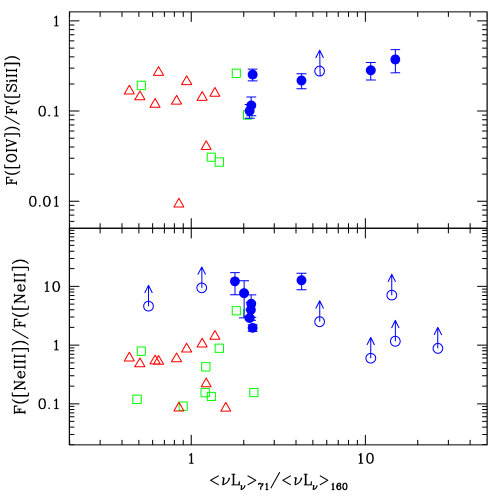
Figure 9: [Ne iii]/[Ne ii]/ (lower panel) and [O iv]/[Si ii]  (upper) plotted against MIPS ratio $\langle\nu{\rm L}_{\nu}\rangle$₇₁/$\langle\nu{\rm L}_{\nu}\rangle$₁₆₀. As in Fig. 4, BCDs are shown as filled circles, and the SINGS galaxies (Dale et al., 2009) as open squares (Hii region-nuclei) and open triangles (AGN). In the upper panel, the $3\sigma$ [Si ii] upper limit (with [O iv] detection) is shown as an open circle.

Using the 71/160µm luminosity ratio ($\langle\nu{\rm L}_{\nu}(71)\rangle/\langle\nu{\rm L}_{\nu}(160)\rangle$) as a tracer of the ISRF intensity, we next investigate whether any of the FS line ratios, indicators of the ISRF hardness as shown above, are correlated with it. Figure 9 shows the [Ne iii]/[Ne ii] and [O iv]/[Si ii] line ratios as a function of the 71/160µm ratio; SINGS galaxies are also plotted combining data from Dale et al. (2007) and Dale et al. (2009). The [Ne iii]/[Ne ii] flux ratio shows no correlation, although there is a weak one in the BCD sample alone (at the $\;\buildrel>\over{\sim}\;$97% confidence level) for [O iv]/[Si ii]; the [O iv]/[Si ii] ratio is larger for warmer large grains. In the SINGS sample, most of the highest [Ne iii]/[Ne ii] and [O iv]/[Si ii] flux ratios are associated with AGN, so any correlation could be masked by AGN high-excitation emission-line ratios in galaxies with a relatively low-intensity ISRF. In any case, we conclude that the hardness of the ISRF, as measured by [O iv]/[Si ii] is weakly related to its intensity, as traced by the 71/160µm luminosity ratio. In lower metallicity BCDs, the ISRF tends to be both harder and more intense.

To summarize, in our low-metallicity BCD sample, the [O iv]/[Si ii] ratio is correlated with Heii/H$\beta$, 12$+$log(O/H), and the large-grain dust temperature (71/160µm ratio). This implies that star-forming galaxies with a lower nebular metallicity as compared to more metal-rich galaxies, generally possess an ISRF which is both harder, as indicated by higher [O iv]/[Si ii] or Heii/H$\beta$ flux ratios, and more intense as indicated by a larger 71/160µm luminosity ratio. The relatively large scatter in some of these relations, and the “plateau-like” behavior of others, implies that these quantities do not depend on only one parameter, but that many parameters are involved. The ISRFs in the SINGS galaxies are of considerably lower intensity than those generally found in BCDs. This is probably because the star-forming regions are more extended, less extreme, and have a lower ionization parameter $Q$. Such factors are probably as important as ISRF hardness and metallicity.

4.3 Electron densities

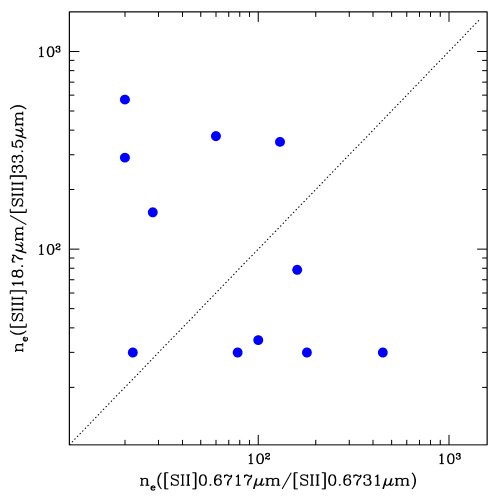
Figure 10: Electron densities $n_{\rm e}$ derived from IR [S iii] line ratios vs. those inferred from optical [S iii] line ratios. The dotted line denotes equality.

We have derived electron densities $n_{\rm e}$ in the ionized gas from the ratio of the temperature-insensitive [S iii] IR lines (Draine, 2009). Fig. 10 shows these densities as compared with those derived using the optical [S ii] $\lambda$6717/$\lambda$6731 ratio. If the IR emission were to originate in regions suffering from higher extinction than the optical regions, we might expect the IR $n_{\rm e}$ to be higher than those derived from the optical lines. Fig. 10 shows that this is true for some BCDs, but not all. On the contrary, a few galaxies show higher optical than IR densities. The reason for this behavior is unclear; beam dilution could play a role since the IRS aperture is several times larger than the optical one and thus includes lower density outer regions.

In the optical, high-ionization radiation responsible for ions such as [Ne v] is found to be associated with extremely massive compact super star clusters and high optical densities (Thuan & Izotov, 2005). The idea that compact star-forming regions were associated with higher electron densities $n_{\rm e}$ was first proposed on theoretical grounds by Hirashita & Hunt (2004). The size-density correlation in Hii regions in which smaller regions are denser is observed over six orders of magnitude from Galactic objects to distant BCDs (Hunt & Hirashita, 2009). If fast radiative shocks were responsible for the ionizing radiation as proposed by Thuan & Izotov (2005), then we would expect such processes to be more efficient at high densities. However, in the current BCD sample, only two (three) of 7 (9) galaxies with a 3$\sigma$ (2$\sigma$) [O iv] detection has a $n_{\rm e}$ above the low-density limit of $\sim$30 cm^-3. The electron densities as derived from the [S iii] IR lines are apparently not correlated with the hardness of the ISRF, as measured by [O iv]/[Si ii]. One reason for this non-correlation may be that [O iv]  with an ionization potential of 54.9 eV is not probing sufficiently high ionization energies (the [Ne v] line has an ionization potential of 97.1 eV). Another reason may be that the [S iii] IR lines arise from a region that is less dense than the [O iv] region. More work on a larger sample is needed to explore the connection between density, geometry, and the ISRF.

4.4 [O iv] and [Fe ii] in BCDs

The two FS lines [O iv] and [Fe ii] lie at adjacent wavelengths ($\Delta\lambda\,=\,$0.098µm) near 26.0 µm. They are, however, sufficiently separated to be resolved by LH IRS spectra. While [O iv] traces high-excitation gas, [Fe ii] has an ionization potential of 7.9 eV, more similar to [Si ii] (see $\S$4.5). Both lines may be excited by photoionization and shocks (Lutz et al., 1998; O’Halloran et al., 2006; Allen et al., 2008). By fitting the two lines with Gaussian profiles, we are able to deblend them in our spectra. We detect [O iv] at 3$\sigma$ in 7/22 observed galaxies, but [Fe ii] at 3$\sigma$ in only Mrk 5 and Mrk 996 (see Fig. 2). At low metallicity, [O iv] emission is almost 4 times as common as [Fe ii] (32% vs. 9%).

This conclusion contrasts with the findings of O’Halloran et al. (2006, 2008). Using Spitzer archival IRS data, they have published 26.0 µm [Fe ii] fluxes for a sample of starbursts, including the 22 BCDs reported here. While the uncertainties in the spectra estimated by us (see $\S$3) are generally more conservative than those reported by O’Halloran et al. (2008), these authors find [Fe ii] emission in all objects, but report no [O iv] emission. The [Fe ii] emission fluxes they find are also larger than ours, suggesting contamination from the [O iv] emission. Figure 2 shows the identifications of the two lines; it is evident that the [Fe ii] flux can be securely measured only when [O iv] is taken into account. No spectra are shown by O’Halloran et al. (2008), so we cannot directly compare their line identifications with ours to resolve the source of discrepancy.

4.5 [Si ii] Emission

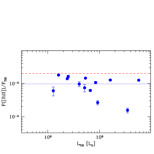
Figure 11: [Si ii] emission normalized by and plotted against TIR. The blue dotted horizontal line indicates the BCD mean, without any MIPS ULs and without UM 311 ($L_{\rm TIR}$$\sim 3\times 10^{9}$$L_{\odot}$), since its TIR is overestimated because of crowding (see text). The red dashed line corresponds to the mean for the SINGS sample (Roussel et al., 2007).

The [Si ii] line is detected in more than half the BCDs in our sample. At an ionization potential of only 8.2 eV, [Si ii] traces the neutral gas, rather than the more highly excited ionized gas traced by the neon, sulfur, and oxygen lines. Figure 11 shows the [Si ii] emission normalized to the TIR luminosity. The mean [Si ii]/TIR ratio is more than a factor of two lower than that of the SINGS galaxies, $8\times 10^{-4}$ versus $2\times 10^{-3}$ (compare the dotted and dashed horizontal lines in Fig. 11). This slight difference is probably due to the lower metal abundance of the BCDs, and the consequently less efficient cooling of the gas through FS lines. It could also be due to a more intense ISRF, and thus a lower Si⁺ abundance. In any case, the ratio of [Si ii] emission to $L_{\rm TIR}$ is relatively constant with luminosity (excluding UM 311 as discussed previously). These considerations suggest that the [Si ii] line is an efficient coolant, comparable to the [Cii] line (e.g., Malhotra et al., 1997), and could be used as a proxy for $L_{\rm TIR}$ to within a factor of two, even at low metallicities.

5 Aromatic Features

The wealth of spectral data obtained by ISO combined with much theoretical work and laboratory measurements has shown convincingly that aromatic features are associated with stochastic or single-photon emission from large molecules called polycyclic aromatic hydrocarbons or PAHs (Joblin et al., 1995; Verstraete et al., 2001; Hony et al., 2001; Peeters et al., 2002; van Diedenhoven et al., 2004; Peeters et al., 2004a; Bauschlicher et al., 2008, 2009). PAH emission dominates the mid-infrared spectra of star-forming galaxies (Brandl et al., 2006; Smith et al., 2007), and contributes importantly to their IR energy budget. Through the photoelectric effect, PAHs heat the gas in the ISM (e.g., Hollenbach & Tielens, 1997), thereby reinforcing the coupling of the gas and dust components. Because they are so dominant in the MIR spectral range, PAHs have been used to identify galaxies with intense star formation at redshifts of $\sim 2-3$, and to estimate their bolometric luminosities (e.g., Houck et al., 2007; Weedman & Houck, 2008; Dey et al., 2008).

In most star-forming galaxies, PAH emission shows a surprisingly narrow range of properties, well characterized by a “standard set” of features with fixed wavelengths and FWHMs (Smith et al., 2007). However, first ISO and later Spitzer have shown that metal-poor star-forming galaxies are deficient in PAH emission (Thuan, Sauvage, & Madden, 1999; Engelbracht et al., 2005; Madden et al., 2006; Wu et al., 2006; Engelbracht et al., 2008). Although it has generally been concluded that the reason for this deficiency is low metallicity, it is not yet clear whether it is the metallicity directly, or rather the indirect effects of a low metallicity environment. In the first case, there would be a consequent lack of raw material (carbon and nitrogen) with which to form PAHs; in the second, the increased ISRF hardness or intensity would lead to their destruction. Here, we examine in detail the PAH emission in our sample to examine this question, and show for the first time that some PAHs can survive even in extremely metal-poor environments.

5.1 PAH Properties at Low Metallicity

The 7.7 µm blend is the most common PAH feature in our sample, being detected in 15 of 22 objects. The 7.7 µm feature is also the strongest one, comprising on average 49% of the total PAH power. The remaining PAHs are significantly weaker, and less frequently detected: 13 BCDs show the 11.3 µm blend, 9 the 8.6 µm feature, and 7 have a detection of the 6.2 µm PAH. No 17 µm PAH features were detected, and only Mrk 1329 showed a significant detection at 16.4 µm. The 6.2, 7.7, 8.6, 11.3, and 12.6 µm features by themselves constitute $\sim$72% of the total PAH power in BCDs (see Table 3); the SINGS sample has about $\sim$85% of the total PAH power in these features (Smith et al., 2007). Similarly to the SINGS galaxies, other weaker features (not listed in Table 3) which contribute to the PAH luminosity include the 5.7, 6.6, 6.7, 8.3, 10.6, and 10.8 µm features. In our sample, these features comprise roughly 28% of the PAH luminosity, but in SINGS galaxies, only 15%. Part of the reason for this difference may be the difficulty in detecting long-wavelength PAHs in BCDs; only 1 BCD has the 16.4 µm feature detected, while in SINGS galaxies the 16-17 µm blend makes up $\sim$6% of the total PAH power.

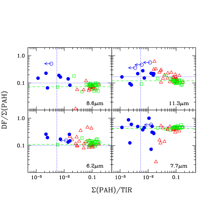
Figure 12: PAH strengths relative to total PAH luminosity vs. the total PAH power normalized to TIR. The four panels show the the following dust features (DF): 6.2 µm (bottom left), 7.7 µm (bottom right), 8.6 µm (top left), 11.3 (top right) µm features. BCDs are plotted as filled (blue) circles, with TIR lower limits shown as open circles; the TIR lower limits do not affect the vertical axis, only the placement along the horizontal one. Open (green) squares correspond to SINGS HII nuclei, and open (red) triangles to SINGS AGN (Smith et al., 2007). The horizontal dashed lines give the SINGS sample medians (Smith et al., 2007), and the dotted ones the means for the BCD sample, taking into account all objects with 7.7 µm detections. The vertical dotted line corresponds to the BCD mean PAH power normalized to TIR.

The fractional power of the four strongest features relative to the total PAH luminosity is illustrated in Figure 12. The horizontal lines in each panel correspond to the SINGS medians (dashed) and the BCD means (dotted). The BCD means are calculated taking into account all galaxies with 7.7 µm detections; thus they are a sort of weighted average which considers frequency of detection together with intensity. This is the reason that the mean for the 6.2 µm PAH lies below most of the BCD data points: that feature was detected only in 7 galaxies, while the other features in Fig. 12 were detected with a frequency more similar to the 7.7 µm PAH. The relative PAH fractions for the BCD and SINGS 6.2 and 7.7 µm features are virtually indistinguishable: 0.10 vs. 0.11 for 6.2 µm, and 0.49 vs. 0.42 for 7.7 µm (Smith et al., 2007). However, for the longer wavelength PAHs at 8.6 and 11.3 µm, the BCD fractions are $\;\buildrel>\over{\sim}\;$ 40% larger: 0.10 vs. 0.07 (8.6) and 0.17 vs. 0.12 (11.3). Although there is considerable scatter, the BCD mean PAH relative fractions for these features tend to exceed even the 10 to 90th percentile spreads of the SINGS galaxies.

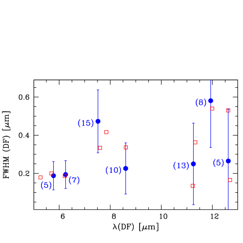
Figure 13: Median Drude profile widths (FWHM) and central wavelengths for seven aromatic features detected ($\lower 2.15277pt\hbox{$\;\buildrel>\over{\sim}\;$}3\sigma$) in our sample. The error bars are the standard deviations of the measurements, and the numbers in parentheses are the numbers of BCDs with significant detections. Open squares correspond to SINGS sample means (Smith et al., 2007).

Figure 13 shows the mean Drude profile widths and central wavelengths of six aromatic features detected at $\lower 2.15277pt\hbox{$\;\buildrel>\over{\sim}\;$}3\sigma$ in our sample; the numbers of BCDs with each feature are given in parentheses. The analogous quantities for the SINGS galaxies are also plotted. In no case, were the PAHFIT profiles fixed to the SINGS galaxy parameters able to fit the BCD data; every BCD was better fitted by allowing the Drude profile widths (FWHMs) and central wavelengths to vary. In some cases, the differences between the $\chi_{\nu}^{2}$ with the SINGS “standard” profile parameters and the best-fit parameters were small, $\;\buildrel<\over{\sim}\;$15%; but in others, the improvement of $\chi_{\nu}^{2}$ was almost a factor of 2. The only systematic difference between the two samples is the narrower profile width for the 8.6 µm feature; only the very broadest BCD profiles are as broad as those in more metal-rich systems.

The larger relative intensities of the 8.6 and 11.3 µm feature in BCDs and the narrow profile width of the 8.6 µm PAH could be due to a different size distribution of PAH populations at low metal abundances. Bauschlicher et al. (2008) find that the 8.6 µm band arises from large PAHs, with $N_{\rm min}\lower 2.15277pt\hbox{$\;\buildrel>\over{\sim}\;$}$ 100 carbon atoms. Hence, they suggest that the relative intensity of the 8.6 µm band can be taken as an indicator of the relative amounts of large and small PAHs in a given population. The large 8.6 µm intensity relative to total PAH power in BCDs could be a signature of fewer small PAHs (or more larger ones) at low metallicity. The relative lack of small PAHs could also explain the low detection rate of the 6.2 µm feature, since most of its intensity comes from PAHs with less than 100 C atoms (Schutte et al., 1993; Hudgins et al., 2005). The size of a PAH molecule grows with the number of carbon atoms in it (e.g., Draine & Li, 2007). For a given maximum number of carbon atoms $N_{\rm max}$, a larger minimum number $N_{\rm min}$ theoretically gives narrower profiles (Joblin et al., 1995; Verstraete et al., 2001). Although fitting intrinsically asymmetric PAH profiles by symmetric Drude profiles in PAHFIT is a simplification, the narrower width of the 8.6 µm feature could be a signature of relatively larger PAHs at low metallicity. The difference disappears at 7.6 µm and is less pronounced at longer wavelengths than 8.6 µm because both small and large PAH sizes contribute to these bands (Schutte et al., 1993; Peeters et al., 2002; van Diedenhoven et al., 2004; Bauschlicher et al., 2009).

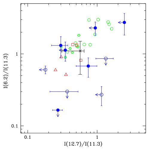
Figure 14: The integrated flux in the PAH features at 6.2 µm, 11.2 µm, and 12.7 µm, plotted in two sets of ratios: 6.2/11.2 vs. 12.7/11.2. Only those BCDs with at least one ratio with 11.2 µm are shown: filled (blue) circles correspond to those BCDs with 12$+$log(O/H)$\geq$8.1; open ones to those objects with lower metallicities. The other data are taken from Hony et al. (2001) and correspond to planetary nebulae (PNe, open red triangles), reflection nebulae (RNe, open red squares), intermediate-mass star-forming regions (six-sided open green stars), and Hii regions (open green hexagons). The SINGS average is shown as a (black) $\times$, with error bars reporting standard deviations over the sample (Smith et al., 2007).

Another indication that low-metallicity BCDs may be lacking the smallest size PAHs comes from a correlation analysis. In a detailed study of Galactic Hii regions, young stellar objects, reflection and planetary nebulae (RNe, PNe), and evolved stars, Hony et al. (2001) found only a few correlations among PAH features. One of these is between 6.2 and the 12.7 µm emission, which arises from the CC stretch mode in ionized PAHs, in contrast to the 11.3 µm band which is attributed to the neutral CH out-of-plane bending mode (Hony et al., 2001; Peeters et al., 2002). The comparison between the 6.2/11.3 and 12.7/11.3 flux ratios is shown for our sample of BCDs in Fig. 14; we show galaxies with $\lower 2.15277pt\hbox{$\;\buildrel>\over{\sim}\;$}3\sigma$ detections in at least two features. With the exception of Mrk 1315, galaxies with 6.2 µm PAH detections and 12$+$log(O/H)$\geq$8.1 (filled circles) are similar to the Hii regions studied by Hony et al. (2001). On the other hand, BCDs with lower O/H occupy a region of the plot with small 6.2/11.3 ratios. Although the statistics are poor, small 6.2/11.3 are found for most of the lowest-metallicity BCDs. They lie in the same region as the RNe and PNe studied by Hony et al. (2001). Because the 11.3 µm feature arises from non-adjacent or “solo” CH groups, dominant 11.3 µm emission implies large PAH complexes, with $\;\buildrel>\over{\sim}\;$100-200 carbon atoms and long straight edges (Hony et al., 2001; Bauschlicher et al., 2008, 2009). Moreover, fewer small PAHs reduce the intensity of the 6.2 µm emission, as the bulk of this feature comes from PAHs containing less than 100 C atoms (Schutte et al., 1993; Hudgins et al., 2005). Therefore, small 6.2/11.3 µm band ratios at low metallicites could imply an overall deficit of small PAHs.

A third indication that there is a deficit of small PAHs in a metal-poor ISM is provided by the intensity of the 8.6 µm feature relative to the 7.7 µm blend. As mentioned above, Bauschlicher et al. (2008) find that 8.6 µm band arises from large PAHs, with $N_{\rm min}\lower 2.15277pt\hbox{$\;\buildrel>\over{\sim}\;$}$ 100 carbon atoms. On the other hand, the 7.7 µm feature contains emission from both small and large PAH sizes (Schutte et al., 1993; Peeters et al., 2002; van Diedenhoven et al., 2004). For the 9 BCDs with the 7.7 and 8.6 µm PAH features detected at $\lower 2.15277pt\hbox{$\;\buildrel>\over{\sim}\;$}3\sigma$, the mean 8.6/7.7 flux ratio is 0.48, and the median is 0.33. This ratio is at least double that in the more metal-rich SINGS galaxies, with 8.6/7.7 $\sim$0.18 in the mean, and a range of 0.11$-$0.21 (Smith et al., 2007); 7 of 9 BCDs are outside the upper 90th percentile limit of 0.21. Again, although the number statistics are small, the large 8.6/7.7 µm flux ratios of the PAHs in these low-metallicity BCDs appear to be dominated by the largest complexes.

In summary, there are three different lines of evidence which tentatively suggest that the PAH populations in low-metallicity BCDs are deficient in the smallest sizes ($N_{\rm min}\lower 2.15277pt\hbox{$\;\buildrel<\over{\sim}\;$}$50 C atoms). The IRS spectra show flux ratios typical of the largest PAHs modeled so far, with $N_{\rm min}\lower 2.15277pt\hbox{$\;\buildrel>\over{\sim}\;$}$100 C atoms. Apparently, the ISM environment in the BCD Hii regions is not propitious to the existence of the smallest PAHs and has led to their destruction. Perhaps only the PAH population with the largest complexes can survive the extreme physical conditions in the low-metallicity Hii regions in the BCDs.

5.2 PAHs and the Energy Budget

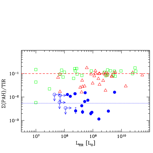
Figure 15: The integrated flux in all the PAH features detected at $\geq 3\sigma$, relative to the total IR flux, plotted against the the total IR flux as described in the text. BCDs are plotted as filled blue circles. The non-AGN SINGS galaxies are plotted as open green squares, and the AGN SINGS galaxies (Seyferts and LINERs) as open red triangles. The blue dotted line shows the median $\Sigma$(PAH)/TIR for our sample of 0.54%; the red dashed line shows the mean $\Sigma$(PAH)/TIR for the SINGS sample of $\sim$10% (Smith et al., 2007).

PAHs emit about 10% of the total infrared power in typical solar metallicity star-forming galaxies (12$+$log(O/H) $\sim$ 8.7-9.0), with a maximum of $\sim$20% (Smith et al., 2007). In our low-metallicity BCD sample, with oxygen abundances 12$+$log(O/H) ranging from 7.4 to 8.3, the fraction of PAH emission ranges from $\sim$0.1% to $\sim$1.6%, with a median (and mean) of $\sim$0.5%. Figure 15 shows how the sum of all $\lower 2.15277pt\hbox{$\;\buildrel>\over{\sim}\;$}3\sigma$ PAH emission features normalized to the total IR luminosity $L_{\rm TIR}$, $\Sigma$(PAH)/TIR, varies as a function of $L_{\rm TIR}$ for our BCD (filled circles) and SINGS galaxies (non-AGN open squares, AGN open triangles) (Smith et al., 2007). For the SINGS galaxies, $L_{\rm TIR}$ has been calculated within the spectral extraction aperture, while for the BCDs, $L_{\rm TIR}$ is taken to be the total luminosity as described in $\S$2.3. Because most of the BCDs are point-like at 24 µm and are generally unresolved with MIPS, this is usually comparable to $L_{\rm TIR}$ within the spectral aperture (see Fig. 2). Were the source sizes larger at 160 µm (e.g., Haro3: Hunt et al., 2006), $L_{\rm TIR}$ could be overestimated, and the PAH fractions somewhat higher. The infrared luminosities $L_{\rm TIR}$ of the SINGS sample vary by a range of more than three orders of magnitude, while the BCD luminosities occupy the middle portion of this range. Figure 15 shows clearly the segregation of the SINGS points, with high $\Sigma$(PAH)/TIR, and the BCD points with low $\Sigma$(PAH)/TIR. The AGN, with intermediate $\Sigma$(PAH)/TIR, lie between the metal-rich star-forming SINGS galaxies and BCDs. Figure 15 also shows that there is no trend of the PAH fraction $\Sigma$(PAH)/TIR with $L_{\rm TIR}$ in either sample.

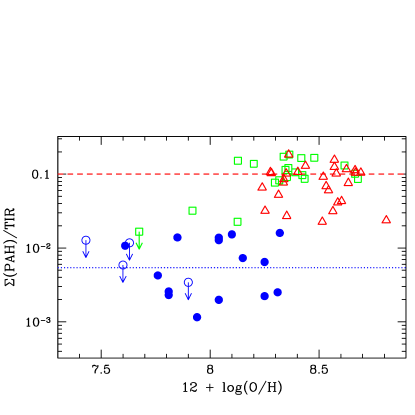
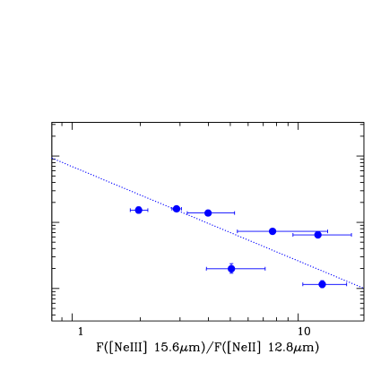
Figure 16: The integrated flux in all the PAH features detected at $\geq 3\sigma$, relative to the total IR flux, plotted against the the oxygen abundance (left panel) and the [Ne iii]/[Ne ii] flux ratio (right). BCDs are shown as filled blue circles, the non-AGN SINGS galaxies as open green squares, and the AGN SINGS galaxies (Seyferts and LINERs) as open red triangles. The horizontal dotted line shows the BCD sample mean $\Sigma$(PAH)/TIR of 0.54%, and the dashed line the SINGS mean of 10%. The right panel shows only those objects with 3$\sigma$ detections or better in each line; the best-fit linear regression is shown as a dotted line.

We might expect the fraction of IR luminosity in PAHs to vary with metallicity. We explore this possibility in the left panel of Fig. 16, where $\Sigma$(PAH)/TIR is plotted against oxygen abundance. Although there is no correlation of PAH fraction with metallicity within the BCD sample, the inclusion of SINGS galaxies does show a trend of increasing PAH fraction with increasing metallicity. We next investigate other physical factors which may control the PAH fraction, such as the ISRF hardness. The right panel of Fig. 16 shows $\Sigma$(PAH)/TIR as a function of the IR neon line ratio, [Ne iii]/[Ne ii] (only those BCDs with at least a 3$\sigma$ detection in the neon lines are shown). As discussed in $\S$4, the [Ne iii]/[Ne ii] ratio is a good tracer of ISRF hardness, up to an intermediate energy range. There is a weak correlation between $\Sigma$(PAH)/TIR and [Ne iii]/[Ne ii], significant at the 95% (one-tailed) confidence level. Thus, over the range in UV energies $\;\buildrel<\over{\sim}\;$41 eV, the fraction of $L_{\rm TIR}$ emerging as PAH emission may depend weakly on the hardness of the ISRF. This suggests that the PAH emission fraction in BCDs is not directly controlled by metallicity, but by the hardness of the radiation field. The latter could also be responsible for the destruction of the smallest PAH particles, as discussed in the previous section. We have checked for a correlation of $\Sigma$(PAH)/TIR with ISRF intensity as measured by $\langle\nu{\rm L}_{\nu}(71)\rangle/\langle\nu{\rm L}_{\nu}(160)\rangle$, but found none.

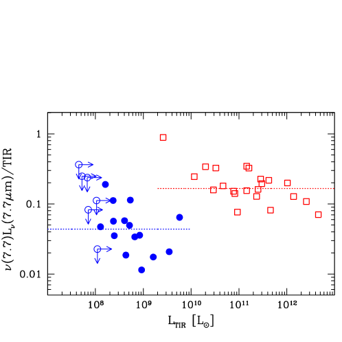
Figure 17: $\nu L_{\nu}$(7.7µm)/TIR plotted again $L_{\rm TIR}$ for the local starbursts in Houck et al. (2007) (shown as open red squares) and the BCDs (filled blue circles). The dotted horizontal line segments correspond to the sample means: 0.044 for the BCDs, and 0.167 for the starbursts.

To conclude our discussion of PAHs and the IR energy budget, we examine the diagnostic proposed by Houck et al. (2007): the quantity $\nu L_{\nu}$(7.7µm), where $L_{\nu}$(7.7 µm) is determined from the flux density at the peak of the 7.7$+$7.8 µm blend, with no correction for the underlying continuum. Because it arises from a range of sizes, the 7.7 µm band is arguably the most reliable PAH diagnostic, as it avoids preferential selection of either small or large PAH populations (Schutte et al., 1993; Peeters et al., 2002). Figure 17 compares $\nu L_{\nu}$(7.7µm)/$L_{\rm TIR}$ for our BCDs with that for a sample of local starbursts (Brandl et al., 2006; Houck et al., 2007). Considering only those BCDs with a 160 µm detection, the BCDs have a mean $\nu L_{\nu}$(7.7µm)/$L_{\rm TIR}$ roughly four times lower than that of the starbursts. The means of the two samples are shown by horizontal dotted lines. Part of this difference may be due to a luminosity effect since the BCDs are more than 100 times less luminous in the mean than the starburst galaxies (see for example the SINGS galaxies in Fig. 15). It may also result from variations of physical conditions in the ISM, since the BCDs with the highest $\nu L_{\nu}$(7.7µm)/$L_{\rm TIR}$ clearly overlap with the range observed in local starbursts that are however much more luminous in $L_{\rm TIR}$.

5.3 PAH Diagnostics for AGN/Starbursts Revisited

Several diagnostics based on IR spectra have been proposed to separate AGN from star-forming regions in galactic nuclei. Previous work has also focused on the comparison of the flux ratios of PAH features and emission line ratios from FS transitions. In this section, we examine our BCD sample in the context of such diagnostics and assess their usefulness in the low metallicity regime.

5.3.1 7.7/11.3 µm Band Ratios

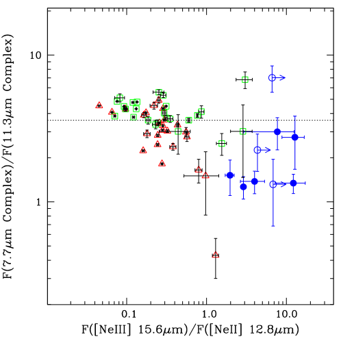
Figure 18: The ratios of the 7.7/11.3 µm bands plotted against [Ne iii]/[Ne ii]. BCDs with $\lower 2.15277pt\hbox{$\;\buildrel>\over{\sim}\;$}3\sigma$ detections are shown as filled blue circles, SINGS AGN as open red triangles, and SINGS HII nuclei as open green squares. The mean 7.7/11.3 µm ratio for the SINGS sample is shown as a horizontal dotted line (Smith et al., 2007).

We saw in the previous section that the total PAH fraction $\Sigma$(PAH)/$L_{\rm TIR}$ is correlated with the IR neon ratio [Ne iii]/[Ne ii] (Fig. 16). Here, following Smith et al. (2007), we examine the variations of the 7.7/11.3 µm band ratios with [Ne iii]/[Ne ii] for both the BCD and SINGS samples as shown in Fig. 18. Among the SINGS galaxies, there is a weak correlation, mostly for AGN, in the sense that a smaller 7.7/11.3 ratio is associated with a larger [Ne iii]/[Ne ii]ratio (e.g., Smith et al., 2007). The BCDs extend the correlation to considerably higher neon ratios (by one order of magnitude), that is to harder ISRFs. The plot shows that the radiation fields in the low metallicity BCDs can be as extreme as those in the SINGS AGN. Such hard, intense ISRFs could suppress the ionized 7.7 µm feature, relative to the neutral 11.3 µm feature. This may be due to the dominant contribution of large PAHs to the 11.3 µm band, as compared to the mixed size distribution thought to be responsible for the 7.7 µm band; the small PAH molecules contributing to the 7.7 µm emission could be destroyed while the large PAH molecules responsible for the 11.3 µm emission are not (see $\S$5.1).

5.3.2 AGN/Starburst Diagnostics

Because a hard, intense radiation field changes the PAH properties, a deficit of PAH emission, combined with FS line indicators of excitation, has often been used as a AGN diagnostic in solar metallicity star-forming galaxies. However, we have seen above that the radiation fields in low metallicity BCDs can be just as intense as those in AGN (see Fig. 18), possibly destroying the smallest PAHs. Thus a PAH emission deficit may not necessarily be a reliable diagnostic for AGN.

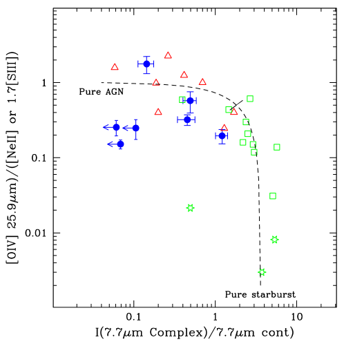
Figure 19: [O iv][Ne ii] (or 1.7$\times$33.5µm [S iii]) vs. the strength of the 7.7 µm PAH feature. The data for starburst galaxies, ULIRGs, and AGN are taken from Genzel et al. (1998), and are marked by green open stars, green open squares, and red open triangles, respectively. Our BCDs as filled blue circles, with upper limits for the PAH features shown by left-pointing arrows; only the (8) BCDs with $\lower 2.15277pt\hbox{$\;\buildrel>\over{\sim}\;$}3\sigma$ [O iv] detections are shown. The “mixing curve” shown by a dashed line is made following Genzel et al. (1998); various fractions of total luminosity in an AGN and a starburst are combined, assuming a pure AGN has [O iv]/[Ne ii]/ $\sim$1, PAH strength $\sim$0.04, and a pure starburst [O iv][Ne ii]/ $\sim$0.002, PAH strength $\sim$3.6. The 50% mark is shown as a line segment along the mixing curve.

We compare our BCD sample with AGN taken from Genzel et al. (1998), using the diagnostics proposed by the latter authors and Laurent et al. (2000). Figure 19 shows the [O iv]/[Ne ii] ratio (or 1.7$\times$33.5µm [S iii], see Genzel et al., 1998) as a function of the “strength” of the 7.7 µm PAH band. [O iv]/[Ne ii] is another measure of ISRF hardness (see $\S$4 where we used [O iv]/[Si ii]). The “strength” of the 7.7 µm PAH feature was determined by estimating the continuum level between 5 and 14 µm  and dividing the PAH flux by this level; this method is the same as that used by Genzel et al. (1998), so we preferred it to the simpler equivalent width measurement given by PAHFIT. For metal-rich systems, plotting these two ratios against one another results in a clear distinction between star-forming galaxies (stars and squares) and AGN (triangles), the latter having a higher [O iv]/[Ne ii] ratio and a weaker 7.7 µm PAH feature than the former. However, the situation for the BCDs in our sample is different. They do not fall in the star-forming but rather closer to the AGN region. The starburst with the highest [O iv] fraction in the Genzel et al. (1998) sample is NGC 5253 (open star symbol), a BCD-like galaxy with an oxygen abundance of 12$+$log(O/H)$\sim$8.2 (Kobulnicky et al., 1999). Two BCDs in our sample would have been classified as pure AGN on the basis of this diagnostic diagram. Thus, the strength of [O iv] combined with the 7.7 µm PAH deficit in metal-poor starbursts makes them difficult to distinguish from AGN.

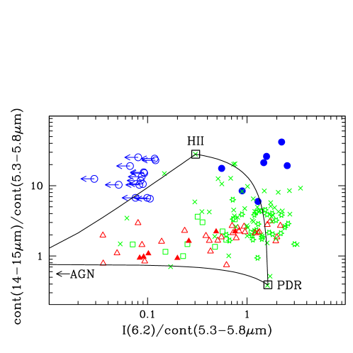
Figure 20: Diagnostic diagram as in Peeters et al. (2004a), adapted from Laurent et al. (2000). The templates for the “mixing” curves are empirical, defined to be the positions of M 17 (Hii region), NGC 7023 (an exposed PDR), and a pure AGN (assumed to have negligible 6.2 µm flux in the PAH band). Data are taken from Peeters et al. (2004a), and include Seyfert 1s (filled red triangles), Seyfert 2s (open red triangles), ULIRGs (open green squares), starburst galaxies (open green stars), and Galactic star-forming regions (green $\times$). Again, BCDs are shown as filled blue circles, with upper limits for the 6.2 µm PAH feature shown as left-pointing arrows.

The second AGN diagnostic diagram often used is illustrated in Fig. 20. This diagnostic, proposed by Laurent et al. (2000), exploits the steeply rising MIR continuum in starbursts, compared to the flatter continua in AGN and quiescent star-forming regions (or PDRs). Most star-forming galaxies have both PDR and Hii region components in their spectra; the PDR component tends to have a flat MIR continuum and be dominated by PAH bands, while the Hii regions have a deficiency of PAHs and a steeply rising MIR continuum from warm dust. To analyze our BCD sample, we have not used the original diagnostic diagram as proposed by Laurent et al. (2000), but a slightly modified version of it as formulated by Peeters et al. (2004a). It differs from the original diagram in the continuum wavelength range that enters in the denominator of the labels on both axes. Fig. 20 plots the 14$-$15 µm continuum against the 6.2 µm PAH feature, both normalized by the 5.3$-$5.8 µm continuum. In this diagram, because of their steep MIR continua, the BCDs (filled circles) are clearly distinguished from the AGN (triangles), ULIRGs (squares), and metal-rich star-forming galaxies (stars), lying above them. A few BCDs are consistent with metal-rich Galactic Hii regions ($\times$), but others are more extreme, both in their steeper continuum slope and in their enhanced PAH strength (or faint 5 µm continuum). The four BCDs with the steepest continua and most enhanced PAH strength are also the most metal-rich galaxies in our sample (Haro 3, Mrk 450, Mrk 1315, and UM 311). We conclude that the AGN/starburst diagnostic diagram proposed by Laurent et al. (2000) based on the continuum MIR slopes of these types of objects effectively separates AGN from starbursts, even at low metallicity.

6 Molecules

A long-standing puzzle of metal-poor star formation has been the apparent lack of cool molecular gas from which to form stars. Numerous attempts to detect carbon monoxide in metal-poor BCDs, with nebular oxygen abundances 12$+$log(O/H)$\;\buildrel<\over{\sim}\;$8.2, have failed. Despite vigorous on-going star formation, there seems to be very little CO in BCDs (Sage et al., 1992; Taylor et al., 1998; Gondhalekar et al., 1998; Barone et al., 2000; Leroy et al., 2005). Intriguingly, 12$+$log(O/H)$\;\buildrel<\over{\sim}\;$8.2 appears to be the same metallicity “threshold” below which PAH emission is thought to be suppressed (Engelbracht et al., 2005; Wu et al., 2006; Madden et al., 2006; Engelbracht et al., 2008). Here we show that warm molecular gas in the form of H₂ does exist at very low metallicity. Our new IRS spectra reveal a variety of H₂ rotational lines, and more than a third of the objects in our sample (8 BCDs) have $\lower 2.15277pt\hbox{$\;\buildrel>\over{\sim}\;$}3\sigma$ detections in one or more of the four lowest-order transitions of H₂.

6.1 H₂ Emission

Rotational transitions of H₂ are important diagnostics of the warm neutral phase of the ISM, at temperatures between $\sim$100 and 1000 K. These transitions, observable from space between 5 and 28 µm, are a main coolant of the warm molecular component. Massive stars are the main source of excitation (Hollenbach & Tielens, 1997), as H₂ molecules can be pumped by non-ionizing far-ultraviolet (FUV) photons into excited states. They then return to the ground state through fluorescence or collisional deexcitation. The pure fluorescence mechanism is likely to be responsible for the near-infrared roto-vibrational transitions (e.g., Puxley et al., 1988), because of the higher critical densities needed for collisional deexcitation. Critical densities of the lower-order rotational transitions are sufficiently low ($\lower 2.15277pt\hbox{$\;\buildrel<\over{\sim}\;$}\,10^{3}$ cm^-3 for S(0) to S(3)) that the lower rotational levels should be thermalized. For the pure rotational H₂ transitions studied here, $\Delta v$ is 0; we will refer to the $\Delta J$ series of rotational transitions as S(0), S(1), …, S(7) (for a complete tabulation, see Roussel et al., 2007).

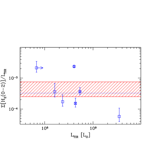
Figure 21: Sum of S(0) to S(2) H₂ luminosity normalized by and plotted against TIR. All detections with $\lower 2.15277pt\hbox{$\;\buildrel>\over{\sim}\;$}2\sigma$ are plotted; a $\times$ denotes the 3$\sigma$ detections. Different symbols distinguish which H₂ lines are considered in the sum: Mrk 996 with S(0) and S(1), and CGCG $005-027$ with S(1) and S(2), are shown by open circles; the remaining BCDs with only S(1) or S(2) by open squares. The red hatched area shows the range for SINGS galaxies (Roussel et al., 2007), and the blue dotted horizontal line indicates the BCD mean, without UM 311 ($L_{\rm TIR}$$\sim 3\times 10^{9}$$L_{\odot}$) because of the likely overestimate of its TIR because of source crowding (see text).

We first examine the H₂ emission in terms of its contribution to the energy budget in the neutral ISM. Following Roussel et al. (2007), we use the sum of the S(0) to S(2) transitions to assess H₂ cooling. The bulk of H₂ cooling occurs through these lines. Figure 21 shows the sum of the S(0) to S(2) H₂ emission, normalized to the total IR luminosity, $L_{\rm TIR}$. As before, both the SINGS and BCD samples are plotted; the SINGS galaxies are confined to the hatched region. The $\Sigma[{\rm H}_{2}(0-2)]$/TIR ratios range from $1\times 10^{-4}$ to $2\times 10^{-3}$, with a mean of $\sim 5\times 10^{-4}$ for the BCD sample . The $\Sigma[{\rm H}_{2}(0-2)]$/TIR for the SINGS galaxies range from $2.5\times 10^{-4}$ to $7.5\times 10^{-4}$ (Roussel et al., 2007). Relative to $L_{\rm TIR}$, the warm molecular content of the BCDs is comparable to that of the SINGS galaxies.

Because warm H₂ emission originates in PDRs, the UV-illuminated parts of molecular clouds, H₂ and PAH emission should be related, since both species are excited by UV photons. Although our sample contains too few points to explore such a correlation, the mean ratio of $\Sigma[{\rm H}_{2}(0-2)]$ to $\Sigma$(PAH) of $\sim$6% is roughly ten times larger than that for the SINGS galaxies (Roussel et al., 2007). Because the H₂ emission of BCDs, relative to TIR, is similar to the SINGS sample, this difference arises mainly from the deficit in PAH emission at low metallicites. Models show that the intensity of rotational transitions of H₂ peaks inside molecular clouds at extinctions A_V$\sim$2 (Hollenbach & Tielens, 1997), while PAHs are expected to be excited predominantly on the cloud surface layers. Deeper into the cloud, densities are higher and temperatures lower, and PAHs would be coagulated onto grain mantles (Boulanger et al., 1990). The similarity of H₂/$L_{\rm TIR}$ over a wide range of metallicity implies that H₂ might be somewhat self-shielded in BCDs. Although PAHs can survive the impact of FUV photons with energies between $\sim$11 and 13.6 eV, H₂ would be dissociated without self-shielding. It is also difficult to understand how, without self-shielding, the H₂ could survive the intense UV radiation field in low metallicity BCDs that is destroying the smallest PAHs (see $\S$5.1).

Although more than a third of our sample show definite low-order H₂ emission in their IRS spectra, all attempts to detect H₂ in BCDs in UV FUSE absorption spectra have failed (Thuan et al., 2005). The absence of H₂ absorption lines in FUSE spectra implies that the warm H₂ detected through IR emission must be quite clumpy. The FUSE observations are not sensitive to such a clumpy H₂ distribution because they can only probe the transparent UV sight lines, not being able to penetrate dense clouds with $N(H_{2})\lower 2.15277pt\hbox{$\;\buildrel>\over{\sim}\;$}10^{20}$ cm^-2 (Hoopes et al., 2004).

6.1.1 H₂ Excitation Temperatures

Excitation diagrams for the H₂ lines help infer the excitation temperatures for molecular hydrogen. For four galaxies in our sample, there were sufficient data to construct excitation diagrams. These diagrams show, as a function of the upper level energy $kT_{i}$, the natural logarithm of the column density of the species $N_{i}$ in the upper level of each transition, divided by the statistical weight, $g_{i}$. Assuming local thermodynamic equilibrium (LTE), the total column density N_tot then follows from the Boltzmann equation:

$$\frac{N_{i}}{N_{\rm tot}}\,=\,\frac{g_{i}}{Z(T_{ex})}\exp\left(-\frac{T_{i}}{T_{ex}}\right)$$ (1)

where $T_{ex}$ is the excitation temperature for the $i^{th}$ level, and $Z(T_{ex})$ is the partition function. The statistical weight is given by $g_{i}\,=\,(2I+1)/(2J+1)$; the spin number takes the values $I=0$ for even $J$ (para) transitions, and $I=1$ for odd $J$ (ortho) transitions. Herbst et al. (1996) gives a convenient expression for the partition function: $Z(T_{ex})\,=\,0.0247\,T/[1-\exp(-6000\,{\rm K}/T)]$, valid for temperatures $\;\buildrel>\over{\sim}\;$40 K. The column density for a given transition $N_{i}$ is calculated from the observed H₂ flux $F_{i}$ in that transition:

$$N_{i}\,=\,\frac{F_{i}4\pi}{h\nu_{i}A_{i}\Omega}$$ (2)

where $A_{i}$ is the transition’s spontaneous emission coefficient, $\nu_{i}$ is the frequency of the transition, and $\Omega$ is the beam solid angle.

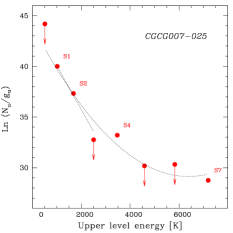
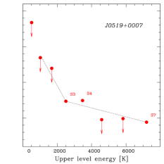
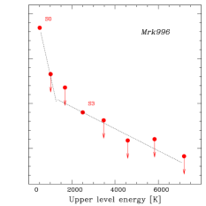
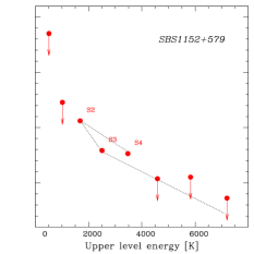
Figure 22: Excitation diagrams for the four BCDs with multiple significant H₂ detections and at least one significant ($\lower 2.15277pt\hbox{$\;\buildrel>\over{\sim}\;$}2.5\sigma$ for SBS 1152$+$579) detection in a low-order transition (see text). 3$\sigma$ upper limits are shown with vertical arrows. The dotted lines correspond to best-fit estimates of the temperature of the line-emitting gas (see text). The parabolic fit for CGCG $005-027$ is an experiment to show the continuity of the data, and thus the continuous range of gas temperatures.

Figure 22 shows the resulting excitation diagrams for the four BCDs which have at least one detection at the 3$\sigma$ level or greater in a low-order transition (except for SBS 1152$+$579 for which we have used 2.5$\sigma$ detections), and at least two other significant ($\lower 2.15277pt\hbox{$\;\buildrel>\over{\sim}\;$}3\sigma$) detections in higher-order lines. Since the inferred column density for a given transition depends on the beam size, we have experimented using different beam sizes of the IRS modules for the various transitions. The main result of this exercise is that the most appropriate beam size is the largest LH beam, equal to 11$\farcs$1$\times$22$\farcs$3. Because the scale of our spectra was ultimately set by the LH background subtraction (see $\S$2), and it was never necessary to multiply by a scaling factor larger than the ratios of the apertures, this is a reasonable conclusion. However, the sources observed at 24 µm with MIPS are either unresolved or only slightly extended, which would imply a slightly different beam dilution for each galaxy at longer wavelengths; applying such a correction would have been highly problematic. Nevertheless, since we have used the IRS point-source flux calibration, this may not be a serious problem, and, because of the way our spectra have been scaled, the excitation diagrams should not be affected significantly by this approximation. With a beam size that is too small, column densities are overestimated and total masses are underestimated. Hence, in Fig. 22, we have taken the most conservative approach for column densities, using the LH beam as discussed above. At the median distance of 21 Mpc for our sources, this corresponds to a region of $\sim$1.6 kpc in diameter.

The excitation temperature of the line-emitting gas is the reciprocal of the slope of the excitation curve; in the absence of fluorescence, this temperature would be the gas kinetic temperature in LTE. Assuming thermal emission, Fig. 22 implies a range of temperatures for the molecular gas. As a crude approximation to the probable continuous temperature distribution of the gas (see the parabolic fit for CGCG $005-027$), we have fitted the data points in each diagram by two linear segments (see also Rigopoulou et al., 2002; Higdon et al., 2006; Roussel et al., 2007). The temperature inferred is a strong function of the set of transitions from which it is derived: lower-order transitions probe lower-temperature gas than the higher-order ones. The implied temperature for the warm gas (from the lower-order transitions) is $\sim$245 K (not considering Mrk 996 at 98 K, the only galaxy with a significant S(0) detection). The temperatures of the hotter molecular component (from the high-order transitions) range from $\sim$820 K to $\sim$1600 K. Considering the transitions from which they are derived, these temperatures are consistent with those found for starbursts (Rigopoulou et al., 2002), SINGS galaxies (Roussel et al., 2007), and ULIRGs (Higdon et al., 2006).

We have not considered any departure from the standard ortho-para ratio of 3 for LTE (e.g., Burton et al., 1992; Roussel et al., 2007). Departure from thermalization of ortho and para levels would be suggested by a non-monotonic increase of inferred excitation temperatures with increasing rotational transition. The temperatures derived from mixed-parity H₂ transitions for the BCDs in our sample are generally consistent, indicating no departure from thermalization for most objects, although Fig. 22 does show some sign of a discrepancy for SBS 1152$+$579. A detailed discussion of this topic at low metallicity is precluded by the paucity of the BCD data presented here.

6.1.2 Column Densities and Gas Masses

Once we have an estimate of the gas temperature for each galaxy, we can derive the H₂ column density and total H₂ mass within the IRS beam. The derived masses and column densities depend on the size of the IRS beam used to relate the observed flux to the column densities. As stated above, we adopted a conservative approach for the column densities, and used the large LH beam, which may give masses that are slightly overestimated.

In our discussion of H₂ column densities and masses, we will consider only those objects in which “secure” temperatures have been derived, i.e. those that have two relatively reliable detections (at the $2.5\sigma$ level or greater) of lower-order transitions. Four objects meet these criteria: CGCG $005-027$, HS 0837$+$4717, Mrk 996, and SBS 1152$+$579. Mrk 996 and CGCG $005-027$ have a total warm (T$\sim$100-120 K) H₂ column density N_H2 $\sim 3\times 10^{21}$cm^-2 or 53 $M_{\odot}$ pc^-2. At a higher temperature of $\sim$340 K, SBS 1152$+$579 has a much lower molecular column density with N_H2 $\sim 3\times 10^{18}$ (0.04 $M_{\odot}$ pc^-2). With a warm/total H₂ fraction of $\sim$5% (Rigopoulou et al., 2002; Roussel et al., 2007), the total molecular column density in SBS 1152$+$579 would be $\;\buildrel<\over{\sim}\;$1 $M_{\odot}$ pc^-2. The column density for HS 0837$+$4717 is more uncertain, because it has only 2.5$\sigma$ detections; the inferred N_H2 is high, $\sim 5\times 10^{21}$ (78 $M_{\odot}$ pc^-2), at a temperature of $\sim$95 K. With the exception of SBS 1152$+$579, the inferred H₂ column densities derived for the BCDs are rather high, compared to the values normally thought to hold for metal-poor galaxies.

Converting to masses, the two most extreme cases are Mrk 996 with a total warm (98 K) H₂ mass in the IRS beam of 1.5$\times 10^{8}$ $M_{\odot}$ and CGCG $005-027$ (at 120 K) of 1.3$\times 10^{8}$ $M_{\odot}$. Compared to the SINGS galaxies, these are rather high warm H₂ masses. There are only three SINGS galaxies with warm ($\;\buildrel>\over{\sim}\;$100 K) H₂ masses which exceed $10^{8}$ $M_{\odot}$, and only one (NGC 7552) with a warm H₂ mass greater than that of Mrk 996. The other BCDs in our sample, with at least one low-order detection have warm (250-470 K) H₂ masses ranging from $4\times 10^{3}$ $M_{\odot}$ (Mrk 209) to $5\times 10^{7}$ $M_{\odot}$ (HS 0837+4717). The median SINGS warm H₂ mass is $\sim 3.4\times 10^{6}$ $M_{\odot}$, and ranges from $\sim 10^{3}$ to $3\times 10^{8}$ $M_{\odot}$ (Roussel et al., 2007). Most of the BCDs have $\lower 2.15277pt\hbox{$\;\buildrel>\over{\sim}\;$}10^{3}$ times more warm H₂ mass than the SINGS low-metallicity galaxies with CO detections, NGC 6822 and NGC 2915 (Roussel et al., 2007).

As stated above, these mass estimates may be overestimates. The true beam size is probably smaller than that of LH. Moreover, molecular hydrogen is not distributed uniformly within that beam but in dense clumps. However, even if we reduced the mass estimates by a factor of five (roughly the difference in beam area between LH and SH), the BCDs’ molecular content would still be quite high. This is contrary to the conventional view that H₂ molecules do not exist in a low-metallicity environment, because of the lack of grains on which to form them. Clearly, metal abundance is not the only factor guiding H₂ formation in low-metallicity BCDs.

Finally, we can compare the warm H₂ mass to that of the neutral atomic gas. According to the star formation models by Krumholz et al. (2009), the H₂ column density of Mrk 966 would correspond to an ISM molecular fraction $\sim$50%, given its metal abundance. Mrk 996 has an Hi mass of 1.5$\times 10^{8}$ $M_{\odot}$(Thuan et al., 1999); thus its H₂ warm mass is comparable to that of its neutral atomic gas mass, in agreement with the theoretical predictions of Krumholz et al. (2009).

Surprisingly, our data suggest that metallicity and H₂ content are not directly linked. Of the four BCDs discussed above with significant low-order H₂ detections, three are below the sample median 12$+$log(O/H) of 7.9. Other factors must play a role in determining the H₂ fraction. In star-forming regions where substantial amounts of dust are concentrated in high-density regions, self-shielding can promote H₂ formation; thus the region can cool more effectively and star-formation rate is enhanced (Hirashita & Hunt, 2004). Thus H₂ content may be more correlated with compactness (size and density) than with metal abundance.

6.2 Water and the Hydroxyl Radical

Our IRS spectra tentatively suggest the presence of H₂O and OH in six objects (see Table 6). Figure 3 shows the $\lower 2.15277pt\hbox{$\;\buildrel>\over{\sim}\;$}3\sigma$ detections of H₂O in three BCDs and OH in four. The H₂O lines at 29.836 µm and 29.885 µm result from rotational transitions of ${\rm H_{2}\,^{16}O}\ 7_{25}-6_{16}$ and $5_{42}-4_{13}$, respectively. The OH emission lines correspond to rotationally excited levels ${}^{2}\Pi_{1/2}\rightarrow^{2}\Pi_{3/2}7/2-5/2$ (28.940 µm), ${}^{2}\Pi_{3/2}19/2-17/2$ (30.346 µm), and ${}^{2}\Pi_{1/2}17/2-15/2$ (30.657 µm). Because some of the spectra also show spurious spectral features near the tentative detections, not associated with known emission lines, these molecule detections are uncertain. Nevertheless, if real, the transitions of “hot” H₂O and OH would be, to the best of our knowledge, the first such detections in extragalactic objects.

Molecular emission from H₂O and OH is perhaps not unexpected, given the physical conditions in some BCDs. H₂O emission from vapor is thought to arise from slow nondissociative, or C-type shocks (e.g., Draine, 1980). In such a situation, at a shock velocity of $\;\buildrel>\over{\sim}\;$10 km s^-1, temperatures would exceed 300 K, and subsequent reactions could rapidly convert all gas-phase oxygen not bound in CO into H₂O (Elitzur & de Jong, 1978). If there is a connection between the dissociative shocks responsible for H₂O vapor emission and the fast radiative shocks possibly responsible for [O iv] emission (see $\S$ 4.4), we would expect both types of emission. Indeed, all three galaxies with H₂O emission in our sample also show $\lower 2.15277pt\hbox{$\;\buildrel>\over{\sim}\;$}3\sigma$ [O iv] detections. Nevertheless, to be consistent with the shock scenario for H₂O production, the H₂ density would need to be rather high, $\lower 2.15277pt\hbox{$\;\buildrel>\over{\sim}\;$}10^{5}$cm^-3 (Elitzur & de Jong, 1978). The electron densities in the ionized gas inferred from the [S iii] line ratio ($\S$ 4.3) are considerably smaller than this, but the [O iv] and H₂O emission could arise from different regions that are much denser. We have no way of verifying this condition with the present data. With Herschel, it may be possible to further pursue observations of H₂O vapor at low metallicity, and better understand the necessary physical conditions and formation scenarios for this molecule.

OH emission could be associated with the photo-dissociation of H₂O at photon energies $\;\buildrel>\over{\sim}\;$9 eV, similar to the situation in Galactic outflows (Tappe et al., 2008). Interestingly, the four galaxies with OH detections also have high-order H₂ detections, implying the presence of hot dense gas, thought to be necessary for the neutral reactions leading to OH and H₂O formation (e.g., Hollenbach & McKee, 1979).

7 Summary and Conclusions

We have presented low- and high-resolution IRS spectra, supplemented by IRAC and MIPS measurements, of 22 BCD galaxies, obtained during our Cycle 1 GO Spitzer program (PID 3139). The BCD sample was chosen to span a wide range in oxygen abundance [12$+$log(O/H) between 7.4 and 8.3], and in ISRF hardness as measured by the intensity of the nebular Heii $\lambda$ 4686 emission line relative to H$\beta$. The IRS spectra provide a variety of fine-structure lines, aromatic features, and molecular lines which probe the physical conditions in a metal-poor ISM, and enable a study of the dust properties as function of metallicity, hardness and intensity of the ISRF. We have used the PAHFIT routine to fit simultaneously the spectral features, the underlying continuum and the extinction in the IRS spectra. Fluxes have also been derived by fitting Gaussian profiles to all FS and molecular lines. To place the results for our low-metallicity BCD sample in perspective, we have compared its properties to those of the SINGS galaxy sample (Kennicutt et al., 2003).

We have obtained the following results:

1. The [Ne iii]/[Ne ii] and [S iv]/[S iii] flux ratios are good diagnostics for the softer UV radiation ($\leq$ 40 eV). The [Ne iii]/[Ne ii] ratio depends on metallicity, being 1–2 orders of magnitude greater in our metal-poor BCD sample than in the more metal-rich SINGS galaxies, but the ratio flattens out at 12$+$log(O/H)$\;\buildrel<\over{\sim}\;$8.3. The [O iv]/[Si ii] ratio is an effective measure of harder radiation, and there is a strong correlation of the [O iv]/[Si ii] ratio with oxygen abundance, implying that lower metallicity galaxies have harder ionizing radiation than more metal-rich ones.

2. We detect at 3$\sigma$ [O iv] (ionization potential of 54.9 eV) in 7/22 observed galaxies, but [Fe ii] (ionization potential of 7.9 eV) in only 2. At low metallicity, [O iv] emission is almost 4 times as common as [Fe ii] (32% vs. 9%). This is another indication that the ISRF of low-metallicity galaxies is very hard.

3. Electron densities derived from the IR [S iii] line ratio do not correlate with those inferred from the optical [S ii] ratio, or with the presence of [O iv] emission. We would expect a correlation of [O iv] intensity with electron density, if fast radiative shocks were responsible for the ionizing radiation that produces [O iv]. Perhaps the [S iii] IR lines arise in and probe a region that is less dense than the [O iv] region.

4. The ratio of 71 to 160µm fluxes $\langle\nu{\rm L}_{\nu}(71)\rangle/\langle\nu{\rm L}_{\nu}(160)\rangle$ is sensitive to the temperature of the large (“classical”) grains, and is thus a good indicator of the ISRF intensity. The latter is $\;\buildrel>\over{\sim}\;$5 times greater in the BCDs than in the SINGS galaxy with the most intense ISRF, implying that metal-poor star-forming galaxies have not only a harder ISRF, but also a more intense one than metal-rich galaxies.

5. Two-thirds of the BCDs show PAH features. The flux ratios of the different bands are typical of the largest PAHs modeled so far, with $N_{\rm min}\lower 2.15277pt\hbox{$\;\buildrel>\over{\sim}\;$}$100 C atoms. We interpret these trends as an indication that low-metallicity BCDs contain relatively larger PAHs than more metal-rich environments. Apparently, only these large PAHs are able to survive the hard and intense ISRF in a low-metallicity ISM.

6. The fraction $\Sigma$(PAH)/TIR of PAH emission $\Sigma$(PAH) normalized to the total IR luminosity TIR is considerably smaller in low-metallicity BCDs ($\sim$0.5%) than in the more metal-rich SINGS galaxies ($\sim$10%). At low metallicity, just as in metal-rich galaxies, the PAH fraction of $L_{\rm TIR}$ is constant.

7. There is a good correlation between $\Sigma$(PAH)/TIR and the [Ne iii]/[Ne ii]flux ratio, but not with metallicity or with ISRF intensity. Evidently, over the range in UV energies $\;\buildrel<\over{\sim}\;$41 eV, the fraction of TIR emerging as PAH emission depends on the hardness of the ISRF. This suggests that the PAH fraction in BCDs is not directly controlled by metallicity, but rather by the hardness of the radiation field, also responsible for the destruction of the smallest PAH particles.

8. The hardness of the ISRF in BCDs can be comparable to that in AGN. Because of this, the [O iv]/[Ne ii] flux ratio, often used as a diagnostic to distinguish star-forming galaxies from AGN at solar abundances, cannot play that role in the low-metallicity regime: in the [O iv]/[Ne ii] vs. 7.7 µm PAH band diagnostic diagram, low-metallicity BCDs occupy the same region as metal-rich AGN. On the contrary, the AGN/starburst diagnostic diagram proposed by (Laurent et al., 2000), based on the continuum MIR slopes of these types of objects, does a good job at separating AGN from starbursts, even at low metallicity.

9. Our IRS spectra reveal a variety of H₂ rotational lines, and more than one third of the objects in our sample (8 BCDs) have $\lower 2.15277pt\hbox{$\;\buildrel>\over{\sim}\;$}3\sigma$ detections in one or more of the four lowest-order transitions of H₂. The BCDs contain more H₂ than most SINGS galaxies, relative to $L_{\rm TIR}$. This is quite contrary to the usual assertion that H₂ molecules do not exist in a low-metallicity environment, because of the lack of grains on which to form them. Clearly, metal abundance cannot be the only factor guiding H₂ formation in low-metallicity BCDs.

10. The mean ratio of H₂ to PAH emission is $\sim$6%, or 10 times larger than that for the SINGS galaxies (but comparable to SINGS AGN). This difference arises mainly from the BCD deficit in PAH emission. While PAHs can survive the impact of FUV photons with energies between $\sim$11 and 13.6 eV, H₂ would be dissociated without self-shielding, implying that H₂ could be somewhat self-shielded in BCDs.

11. The mean excitation temperature derived for the warm gas from the lower-order H₂ transitions is $\sim$245 K. The temperatures of the hotter molecular component from the high-order H₂ transitions range from $\sim$820 K (in Mrk 996 and SBS 1152$+$579) to $\sim$1600 K. These temperatures are consistent with those found for starburst SINGS galaxies and ULIRGs. The warm molecular gas masses in our BCDs range from $10^{3}$ to $10^{8}$ $M_{\odot}$, and can be comparable to the neutral hydrogen gas mass.

12. Some of our IRS spectra suggest tentatively the presence of molecules other than H₂, such as H₂O and OH. All three galaxies with H₂O emission also show a $\lower 2.15277pt\hbox{$\;\buildrel>\over{\sim}\;$}3\sigma$ [O iv] line, consistent with a shock scenario for H₂O production. All four galaxies with OH emission also have high-order H₂ detections, implying the presence of hot, dense gas which would favor OH and H₂O formation.

Our IRS data have shown that the ISRF in metal-poor BCDs can be as extreme in hardness as the radiation in AGN. In fact, the deficit of PAH emission at low metallicity and their hard radiation as indicated by [O iv] luminosity would have placed some BCDs as AGN in diagnostic diagrams such as that proposed by Genzel et al. (1998). Our analysis suggests that in the absence of an AGN, low metal abundance is a necessary condition for such extreme fields. However, we have also shown that low metallicity alone does not guarantee an extreme ISRF in terms of hardness and intensity. Other factors such as compactness of the star-forming region must play a role.

We have inferred a deficit of small PAHs, and find that PAH destruction mechanisms are more closely related to the hardness of the radiation field, rather than to metallicity. This is a rather difficult exercise, since most of the [O iv] detections are in galaxies where we have little information on the PAH population, and the converse is also true. Nevertheless, there appears to be a close connection between hardness of the ISRF and the properties of the PAHs; this connection is tighter than that with metallicity. In fact, we find correlations of PAH properties with ISRF hardness, but almost none with metallicity, in spite of the good correlations between hardness tracers and metal abundance.

It is not clear whether the origin of such hard radiation can be stellar. In their detailed modeling of the [O iv] line in Mrk 996, Thuan et al. (2008) ran Costar models by Schaerer & de Koter (1997) using stars with the highest effective temperature (T_eff =53,000 K) and the hardest radiation possible (corresponding to the hottest O3 stars). They failed to reproduce the observed intensity of the [O iv] line by a factor of several. They then considered Wolf-Rayet stars of type WNE-w. According to calculations by Crowther et al. (1999), models for WNE-w stars (early nitrogen Wolf-Rayet stars with weak lines) show a strong ionizing flux above 54.4 eV, in contrast to the WCE and WNL stars, which show negligible fluxes above that energy. The line intensity of [O iv] in Mrk 996 can be reproduced with such a population of WNE-w stars. However, Thuan et al. (2008) do not favor such an hypothesis because WNE-w stars are very rare. Rather, those authors favor fast radiative shocks (Thuan & Izotov, 2005) as the origin of the high-ionization radiation. Shocks are a more realistic expectation in dense compact regions with intense star formation because of SN explosions and massive stellar winds. At low metallicity, the less efficient cooling may intensify the effect of the shock. We postpone an in-depth discussion of the origin of the hard ionizing radiation for the whole of our sample to a future paper. There, we will present detailed photoionization and shock models to account for both optical$+$ IR emission line intensities.

Table 1: Sample Galaxies

Name	Distance	Redshift	12$+$log(O/H)	$c_{H\beta}$	Heii/H$\beta$
CGCG007-025	20.8	0.00483	7.76	0.29	0.0136
HS0837+4717	174.3	0.04195	7.60	0.29	0.0228
HS1442+4250	12.6	0.00211	7.63	0.11	0.0297
HS2236+1344	86.4	0.02062	7.47	0.16	0.0106
Haro3	17.4	0.00323	8.32	0.24	0.0000
IIZw70	21.8	0.00394	8.04	0.21	0.0056
J0519+0007	181.8	0.04476	7.43	0.30	0.0249
Mrk5	15.4	0.00264	8.04	0.42	0.0387
Mrk36	7.6	0.00215	7.81	0.02	0.0244
Mrk209	4.8	0.00094	7.81	0.00	0.0117
Mrk450	15.1	0.00288	8.15	0.14	0.0031
Mrk724	20.0	0.00402	8.03	0.12	0.0000
Mrk996	21.8	0.00541	8.10	0.53	0.0000
Mrk1315	13.1	0.00282	8.25	0.16	0.0000
Mrk1329	13.1	0.00544	8.25	0.16	0.0000
SBS0917+527	35.4	0.00776	7.90	0.09	0.0221
SBS0946+558	25.5	0.00517	8.04	0.18	0.0149
SBS1030+583	35.3	0.00757	7.83	0.00	0.0234
SBS1152+579	74.5	0.01720	7.85	0.26	0.0152
SBS1415+437	11.7	0.00203	7.61	0.00	0.0227
Tol1924-416	38.4	0.00945	7.94	0.26	0.0190
UM311	23.0	0.00559	8.31	0.15	0.0000

Table 2: Short-Wavelength Fine-Structure Lines

Name	[Ar ii]	[Ar iii]	[S iv]	[Ne ii]
	6.985µm	8.991µm	10.511µm	12.814µm
	15.759 eV	27.629 eV	34.830 eV	21.564 eV
CGCG 007$-$025	$\cdots$ (0.33)	0.66 (0.18)	5.98 (0.43)	$\cdots$ (1.29)
Haro 3	3.44 (0.97)	10.60 (1.67)	26.80 (3.70)	27.50 (3.59)
HS 0837$+$4717	$\cdots$ (0.13)	0.28 (0.09)	3.07 (0.41)	$\cdots$ (1.23)
HS 1442$+$4250	$\cdots$ (0.21)	$\cdots$ (0.21)	$\cdots$ (1.60)	$\cdots$ (1.60)
HS 2236$+$1344	$\cdots$ (0.12)	$\cdots$ (0.12)	2.50 (0.56)	$\cdots$ (1.68)
II Zw 70	$\cdots$ (0.72)	$\cdots$ (0.72)	4.03 (0.26)	1.34 (0.30)
J0519$+$0007	$\cdots$ (0.22)	$\cdots$ (0.22)	$\cdots$ (1.17)	$\cdots$ (1.17)
Mrk 5	0.54 (0.08)	0.52 (0.08)	1.64 (0.13)	1.08 (0.13)
Mrk 36	$\cdots$ (0.27)	$\cdots$ (0.27)	2.36 (0.14)	$\cdots$ (0.43)
Mrk 209	1.26 (0.33)	1.58 (0.26)	8.63 (0.18)	$\cdots$ (0.45)
Mrk 450	$\cdots$ (0.21)	1.46 (0.13)	4.45 (0.35)	0.91 (0.29)
Mrk 724	$\cdots$ (0.28)	$\cdots$ (0.28)	3.92 (0.44)	$\cdots$ (1.31)
Mrk 996	$\cdots$ (1.23)	1.87 (0.40)	3.90 (0.32)	4.55 (0.32)
Mrk 1315	0.73 (0.05)	1.36 (0.12)	10.20 (0.48)	$\cdots$ (1.43)
Mrk 1329	$\cdots$ (0.46)	1.80 (0.15)	12.30 (0.27)	1.27 (0.27)
SBS 0917$+$527	$\cdots$ (0.12)	$\cdots$ (0.12)	1.46 (0.12)	$\cdots$ (0.36)
SBS 0946$+$558	$\cdots$ (0.15)	$\cdots$ (0.15)	$\cdots$ (1.63)	$\cdots$ (1.63)
SBS 1030$+$583	$\cdots$ (0.10)	$\cdots$ (0.10)	1.93 (0.59)	$\cdots$ (1.77)
SBS 1152$+$579	$\cdots$ (0.40)	0.92 (0.13)	6.32 (0.12)	$\cdots$ (0.36)
SBS 1415$+$437	$\cdots$ (0.18)	$\cdots$ (0.18)	1.02 (0.22)	$\cdots$ (0.49)
Tol 1924$-$416	$\cdots$ (0.80)	2.56 (0.27)	11.40 (0.34)	1.88 (0.34)
UM 311	$\cdots$ (0.29)	1.71 (0.23)	5.22 (0.69)	$\cdots$ (2.08)

Table 3: Dust Features

Name	DF_5	DF_6	DF_7	DF_8	DF_11	DF_12	DF_17	$\Sigma$PAH
	5.7µm	6.2µm	7.7µm	8.6µm	11.3µm	12.6µm	17µm	Total
							Complex
CGCG 007$-$025	$\cdots$ (0.33)	$\cdots$ (0.33)	6.34 (0.82)	$\cdots$ (0.33)	2.81 (0.51)	$\cdots$ (1.28)	$\cdots$ (0.33)	12.79 (1.12)
	$\cdots$	$\cdots$	7.459	$\cdots$	11.199	$\cdots$
	$\cdots$	$\cdots$	0.470	$\cdots$	0.067	$\cdots$
Haro 3	20.30 (3.53)	101.00 ( 10.60)	188.50 ( 31.85)	56.30 ( 14.40)	148.90 ( 41.95)	111.00 ( 19.30)	$\cdots$ (1.39)	680.60 ( 60.62)
	5.744	6.245	7.808	8.682	11.335	12.673
	0.188	0.194	0.362	0.279	0.544	0.798
HS 0837$+$4717	$\cdots$ (2.91)	$\cdots$ (0.13)	$\cdots$ (0.13)	$\cdots$ (0.13)	1.37 (0.41)	$\cdots$ (1.23)	$\cdots$ (0.13)	2.95 (0.57)
	$\cdots$	$\cdots$	$\cdots$	$\cdots$	11.214	$\cdots$
	$\cdots$	$\cdots$	$\cdots$	$\cdots$	0.090	$\cdots$
HS 1442$+$4250	$\cdots$ (0.21)	0.94 (0.24)	$\cdots$ (0.21)	$\cdots$ (0.57)	3.46 (0.53)	$\cdots$ (1.60)	$\cdots$ (0.21)	6.15 (0.79)
	$\cdots$	6.294	$\cdots$	$\cdots$	11.347	$\cdots$
	$\cdots$	0.094	$\cdots$	$\cdots$	0.545	$\cdots$
HS 2236$+$1344	$\cdots$ (0.12)	$\cdots$ (0.12)	$\cdots$ (0.12)	$\cdots$ (0.12)	$\cdots$ (1.68)	$\cdots$ (1.68)	$\cdots$ (0.12)	$\cdots$ (0.12)
	$\cdots$	$\cdots$	$\cdots$	$\cdots$	$\cdots$	$\cdots$
	$\cdots$	$\cdots$	$\cdots$	$\cdots$	$\cdots$	$\cdots$
II Zw 70	$\cdots$ (0.72)	$\cdots$ (3.78)	10.81 (1.98)	$\cdots$ (0.72)	$\cdots$ (0.66)	$\cdots$ (0.66)	$\cdots$ (0.72)	12.39 (2.03)
	$\cdots$	$\cdots$	7.808	$\cdots$	$\cdots$	$\cdots$
	$\cdots$	$\cdots$	0.207	$\cdots$	$\cdots$	$\cdots$
J0519$+$0007	$\cdots$ (0.22)	$\cdots$ (0.22)	2.45 (0.55)	$\cdots$ (0.22)	$\cdots$ (1.17)	$\cdots$ (1.17)	$\cdots$ (0.22)	4.24 (0.67)
	$\cdots$	$\cdots$	7.405	$\cdots$	$\cdots$	$\cdots$
	$\cdots$	$\cdots$	0.467	$\cdots$	$\cdots$	$\cdots$
Mrk 1315	$\cdots$ (0.15)	3.97 (0.12)	1.91 (0.10)	3.47 (0.48)	1.45 (0.48)	$\cdots$ (1.43)	$\cdots$ (0.15)	15.24 (0.75)
	$\cdots$	6.201	7.500	8.648	11.256	$\cdots$
	$\cdots$	0.279	0.165	0.431	0.088	$\cdots$
Mrk 1329	$\cdots$ (5.70)	$\cdots$ (3.03)	9.31 (0.99)	4.70 (0.87)	6.94 (0.54)	1.89 (0.27)	1.85 (0.49)	24.69 (1.53)
	$\cdots$	$\cdots$	7.520	8.537	11.272	12.627
	$\cdots$	$\cdots$	0.474	0.166	0.541	0.265
Mrk 209	$\cdots$ (2.82)	$\cdots$ (0.32)	$\cdots$ (2.37)	$\cdots$ (0.32)	$\cdots$ (0.45)	$\cdots$ (0.45)	$\cdots$ (0.32)	7.41 (1.28)
	$\cdots$	$\cdots$	$\cdots$	$\cdots$	$\cdots$	$\cdots$
	$\cdots$	$\cdots$	$\cdots$	$\cdots$	$\cdots$	$\cdots$
Mrk 36	$\cdots$ (3.00)	$\cdots$ (0.27)	$\cdots$ (0.27)	$\cdots$ (0.27)	$\cdots$ (0.43)	$\cdots$ (0.43)	$\cdots$ (0.27)	4.73 (1.32)
	$\cdots$	$\cdots$	$\cdots$	$\cdots$	$\cdots$	$\cdots$
	$\cdots$	$\cdots$	$\cdots$	$\cdots$	$\cdots$	$\cdots$
Mrk 450	2.06 (0.25)	6.16 (0.23)	16.40 (1.42)	5.95 (0.85)	5.46 (1.61)	$\cdots$ (0.76)	$\cdots$ (0.21)	36.03 (2.33)
	5.800	6.291	7.520	8.520	11.331	$\cdots$
	0.169	0.283	0.659	0.255	0.388	$\cdots$
Mrk 5	2.17 (0.20)	3.27 (0.14)	7.47 (0.71)	3.45 (0.39)	5.42 (0.64)	$\cdots$ (0.39)	$\cdots$ (0.24)	24.33 (1.08)
	5.791	6.287	7.801	8.708	11.326	$\cdots$
	0.214	0.283	0.281	0.440	0.544	$\cdots$
Mrk 724	$\cdots$ (0.28)	$\cdots$ (0.28)	$\cdots$ (0.28)	$\cdots$ (2.16)	$\cdots$ (1.31)	$\cdots$ (1.31)	$\cdots$ (0.28)	$\cdots$ (0.28)
	$\cdots$	$\cdots$	$\cdots$	$\cdots$	$\cdots$	$\cdots$
	$\cdots$	$\cdots$	$\cdots$	$\cdots$	$\cdots$	$\cdots$
Mrk 996	7.03 (1.45)	15.50 (4.32)	17.90 (4.35)	$\cdots$ (9.63)	11.80 (2.02)	3.53 (0.71)	$\cdots$ (0.66)	60.66 (6.71)
	5.757	6.236	7.493	$\cdots$	11.276	12.684
	0.101	0.179	0.472	$\cdots$	0.250	0.082
SBS 0917$+$527	$\cdots$ (0.12)	$\cdots$ (0.12)	$\cdots$ (0.12)	1.42 (0.23)	1.00 (0.29)	0.37 (0.12)	$\cdots$ (0.12)	2.79 (0.39)
	$\cdots$	$\cdots$	$\cdots$	8.559	11.230	12.601
	$\cdots$	$\cdots$	$\cdots$	0.167	0.539	0.082
SBS 0946$+$558	$\cdots$ (0.15)	$\cdots$ (0.15)	0.89 (0.28)	$\cdots$ (0.15)	2.74 (0.54)	$\cdots$ (1.63)	$\cdots$ (0.15)	12.11 (1.03)
	$\cdots$	$\cdots$	7.520	$\cdots$	11.230	$\cdots$
	$\cdots$	$\cdots$	0.474	$\cdots$	0.539	$\cdots$
SBS 1030$+$583	$\cdots$ (0.10)	$\cdots$ (0.10)	4.75 (0.40)	0.67 (0.14)	$\cdots$ (1.77)	$\cdots$ (1.77)	$\cdots$ (0.10)	5.42 (0.42)
	$\cdots$	$\cdots$	7.520	8.534	$\cdots$	$\cdots$
	$\cdots$	$\cdots$	0.474	0.166	$\cdots$	$\cdots$
SBS 1152$+$579	3.30 (0.70)	$\cdots$ (0.40)	12.20 (0.67)	3.41 (0.46)	$\cdots$ (0.36)	$\cdots$ (0.36)	$\cdots$ (0.40)	24.15 (1.11)
	5.800	$\cdots$	7.520	8.710	$\cdots$	$\cdots$
	0.305	$\cdots$	0.474	0.510	$\cdots$	$\cdots$
SBS 1415$+$437	$\cdots$ (0.18)	$\cdots$ (0.18)	12.84 (0.25)	$\cdots$ (2.04)	$\cdots$ (0.49)	$\cdots$ (0.49)	$\cdots$ (0.18)	12.84 (0.25)
	$\cdots$	$\cdots$	7.782	$\cdots$	$\cdots$	$\cdots$
	$\cdots$	$\cdots$	0.258	$\cdots$	$\cdots$	$\cdots$
Tol 1924$-$416	$\cdots$ (0.80)	$\cdots$ (0.80)	6.39 (1.40)	2.08 (0.62)	2.32 (0.58)	3.09 (0.41)	$\cdots$ (0.80)	13.88 (1.69)
	$\cdots$	$\cdots$	7.507	8.510	11.230	12.643
	$\cdots$	$\cdots$	0.473	0.166	0.180	0.266
UM 311	$\cdots$ (2.37)	12.70 (2.14)	38.76 (5.37)	4.27 (1.29)	5.53 (0.69)	$\cdots$ (2.08)	$\cdots$ (0.29)	64.98 (6.00)
	$\cdots$	6.216	7.822	8.634	11.237	$\cdots$
	$\cdots$	0.163	0.207	0.196	0.067	$\cdots$

Table 4: Long-Wavelength Fine-Structure Lines

Name	[Ne iii]	[S iii]	[O iv]	[Fe ii]	[Fe iii]	[S iii]	[Si ii]	[Ne iii]
	15.555µm	18.713µm	25.890µm	25.988µm	33.038µm	33.481µm	34.815µm	36.014µm
	40.962 eV	23.330 eV	54.934 eV	7.870 eV	16.180 eV	23.330 eV	8.151 eV	40.962 eV
CGCG 007$-$025	5.55 (0.49)	$\cdots$ (1.28)	$\cdots$ (1.49)	$\cdots$ (1.49)	$\cdots$ (1.77)	3.48 (0.67)	2.89 (0.50)	$\cdots$ (1.49)
Haro 3	79.58 (0.27)	40.99 (0.27)	5.38 (0.93)	$\cdots$ (2.80)	27.13 (0.93)	116.41 (0.93)	53.47 (0.93)	12.11 (0.93)
HS 0837$+$4717	1.54 (0.41)	$\cdots$ (1.23)	$\cdots$ (0.92)	$\cdots$ (0.92)	$\cdots$ (0.92)	$\cdots$ (0.92)	$\cdots$ (0.92)	$\cdots$ (0.92)
HS 1442$+$4250	$\cdots$ (1.60)	$\cdots$ (1.60)	$\cdots$ (1.00)	$\cdots$ (1.00)	$\cdots$ (1.00)	$\cdots$ (1.00)	$\cdots$ (1.00)	$\cdots$ (1.00)
HS 2236$+$1344	$\cdots$ (1.86)	$\cdots$ (1.68)	$\cdots$ (0.54)	$\cdots$ (0.54)	$\cdots$ (0.54)	$\cdots$ (0.54)	$\cdots$ (0.54)	$\cdots$ (0.54)
II Zw 70	6.78 (0.35)	3.95 (0.22)	0.77 (0.17)	$\cdots$ (0.60)	$\cdots$ (0.51)	10.09 (0.17)	6.65 (0.53)	$\cdots$ (0.51)
J0519$+$0007	$\cdots$ (1.17)	$\cdots$ (1.17)	$\cdots$ (0.67)	$\cdots$ (0.67)	$\cdots$ (0.67)	$\cdots$ (0.67)	$\cdots$ (0.99)	$\cdots$ (0.67)
Mrk 5	4.31 (0.13)	1.90 (0.13)	$\cdots$ (0.21)	0.24 (0.07)	$\cdots$ (0.21)	5.02 (0.07)	2.45 (0.07)	1.01 (0.07)
Mrk 36	2.70 (0.14)	1.53 (0.14)	1.11 (0.30)	$\cdots$ (0.91)	$\cdots$ (0.91)	2.63 (0.30)	2.97 (0.30)	$\cdots$ (0.91)
Mrk 209	5.57 (0.15)	2.69 (0.15)	1.46 (0.19)	$\cdots$ (0.57)	$\cdots$ (0.57)	5.66 (0.19)	$\cdots$ (0.57)	$\cdots$ (0.57)
Mrk 450	7.00 (1.33)	4.27 (0.25)	$\cdots$ (0.64)	$\cdots$ (0.64)	$\cdots$ (0.64)	5.68 (0.21)	3.03 (0.21)	1.96 (0.21)
Mrk 724	3.98 (0.44)	2.89 (0.44)	$\cdots$ (1.73)	$\cdots$ (1.73)	$\cdots$ (1.73)	$\cdots$ (1.73)	$\cdots$ (1.73)	$\cdots$ (1.73)
Mrk 996	8.95 (0.32)	7.31 (0.32)	1.46 (0.21)	0.96 (0.32)	0.90 (0.21)	16.43 (0.21)	5.75 (0.21)	$\cdots$ (0.63)
Mrk 1315	9.74 (0.48)	5.09 (0.48)	$\cdots$ (0.80)	$\cdots$ (0.80)	$\cdots$ (0.80)	7.26 (0.27)	1.81 (0.27)	$\cdots$ (0.80)
Mrk 1329	15.51 (0.27)	8.07 (0.32)	$\cdots$ (2.10)	$\cdots$ (2.10)	$\cdots$ (2.10)	8.59 (0.70)	2.83 (0.70)	$\cdots$ (2.10)
SBS 0917$+$527	1.00 (0.12)	0.67 (0.12)	$\cdots$ (0.76)	$\cdots$ (0.76)	$\cdots$ (0.76)	$\cdots$ (0.76)	$\cdots$ (0.76)	$\cdots$ (0.76)
SBS 0946$+$558	$\cdots$ (1.63)	$\cdots$ (1.63)	$\cdots$ (0.51)	$\cdots$ (0.51)	$\cdots$ (0.51)	1.56 (0.17)	0.57 (0.17)	$\cdots$ (0.51)
SBS 1030$+$583	$\cdots$ (1.77)	$\cdots$ (1.77)	$\cdots$ (0.83)	$\cdots$ (0.83)	$\cdots$ (0.83)	$\cdots$ (0.83)	$\cdots$ (0.83)	$\cdots$ (0.83)
SBS 1152$+$579	2.45 (0.12)	1.38 (0.14)	$\cdots$ (0.76)	$\cdots$ (0.76)	$\cdots$ (0.76)	2.68 (0.25)	$\cdots$ (0.76)	$\cdots$ (0.76)
SBS 1415$+$437	1.22 (0.16)	1.09 (0.16)	0.61 (0.13)	$\cdots$ (0.40)	$\cdots$ (0.40)	1.41 (0.13)	2.15 (0.13)	$\cdots$ (0.40)
Tol 1924$-$416	23.99 (0.34)	7.40 (0.34)	3.33 (0.61)	$\cdots$ (3.51)	$\cdots$ (1.84)	18.57 (0.61)	15.23 (0.74)	$\cdots$ (6.54)
UM 311	13.75 (0.69)	2.53 (0.69)	$\cdots$ (1.99)	$\cdots$ (1.99)	$\cdots$ (1.99)	$\cdots$ (1.99)	4.01 (0.66)	$\cdots$ (1.99)

Table 5: H₂ Lines

Name	S(7)	S(6)	S(5)	S(4)	S(3)	S(2)	S(1)	S(0)
	5.511µm	6.109µm	6.910µm	8.025µm	9.665µm	12.279µm	17.035µm	28.219µm
CGCG 007$-$025	0.46 (0.13)	$\cdots$ (0.33)	$\cdots$ (0.33)	0.72 (0.21)	$\cdots$ (0.33)	1.67 (0.43)	5.45 (0.43)	$\cdots$ (1.49)
Haro 3	2.03 (0.46)	$\cdots$ (1.39)	$\cdots$ (1.39)	$\cdots$ (1.39)	$\cdots$ (1.39)	$\cdots$ (0.82)	$\cdots$ (0.82)	$\cdots$ (2.80)
HS 0837$+$4717	0.44 (0.19)	$\cdots$ (0.13)	$\cdots$ (0.13)	$\cdots$ (0.13)	0.18 (0.07)	$\cdots$ (1.23)	1.07 (0.41)	$\cdots$ (0.92)
HS 1442$+$4250	0.47 (0.17)	0.41 (0.14)	$\cdots$ (0.21)	$\cdots$ (0.21)	0.17 (0.08)	$\cdots$ (1.60)	$\cdots$ (1.60)	$\cdots$ (1.00)
II Zw 70	$\cdots$ (0.72)	1.53 (0.64)	$\cdots$ (0.72)	1.34 (0.46)	0.69 (0.31)	$\cdots$ (0.66)	$\cdots$ (0.66)	$\cdots$ (0.51)
J0519$+$0007	0.90 (0.17)	$\cdots$ (0.22)	$\cdots$ (0.22)	0.34 (0.11)	0.22 (0.07)	$\cdots$ (1.17)	$\cdots$ (1.17)	$\cdots$ (0.67)
Mrk 5	0.38 (0.08)	0.60 (0.08)	0.35 (0.08)	0.56 (0.08)	$\cdots$ (0.24)	$\cdots$ (0.39)	$\cdots$ (0.39)	$\cdots$ (0.21)
Mrk 36	$\cdots$ (0.27)	$\cdots$ (0.27)	$\cdots$ (0.27)	$\cdots$ (0.27)	0.94 (0.14)	$\cdots$ (0.43)	$\cdots$ (0.43)	$\cdots$ (0.91)
Mrk 209	$\cdots$ (0.32)	$\cdots$ (0.32)	$\cdots$ (0.32)	$\cdots$ (0.32)	0.52 (0.23)	0.49 (0.16)	$\cdots$ (0.45)	$\cdots$ (0.57)
Mrk 450	$\cdots$ (0.21)	0.78 (0.08)	0.58 (0.07)	0.39 (0.18)	0.20 (0.08)	$\cdots$ (0.76)	$\cdots$ (0.76)	$\cdots$ (0.64)
Mrk 996	$\cdots$ (0.66)	$\cdots$ (0.66)	1.19 (0.48)	$\cdots$ (0.66)	1.15 (0.35)	$\cdots$ (0.97)	0.74 (0.32)	0.71 (0.21)
Mrk 1315	$\cdots$ (0.15)	$\cdots$ (0.15)	0.18 (0.05)	$\cdots$ (0.15)	$\cdots$ (0.15)	$\cdots$ (1.43)	$\cdots$ (1.43)	$\cdots$ (0.80)
Mrk 1329	$\cdots$ (0.46)	1.05 (0.21)	$\cdots$ (0.46)	0.78 (0.18)	$\cdots$ (0.46)	$\cdots$ (0.80)	$\cdots$ (0.80)	$\cdots$ (2.10)
SBS 0917$+$527	$\cdots$ (0.12)	$\cdots$ (0.12)	$\cdots$ (0.12)	0.38 (0.16)	$\cdots$ (0.12)	$\cdots$ (0.36)	$\cdots$ (0.36)	$\cdots$ (0.76)
SBS 0946$+$558	$\cdots$ (0.15)	$\cdots$ (0.15)	0.21 (0.05)	$\cdots$ (0.15)	$\cdots$ (0.15)	$\cdots$ (1.63)	$\cdots$ (1.63)	$\cdots$ (0.51)
SBS 1030$+$583	0.53 (0.13)	$\cdots$ (0.10)	$\cdots$ (0.10)	$\cdots$ (0.10)	$\cdots$ (0.10)	$\cdots$ (1.77)	$\cdots$ (1.77)	$\cdots$ (0.83)
SBS 1152$+$579	$\cdots$ (0.40)	$\cdots$ (0.40)	$\cdots$ (0.40)	0.41 (0.15)	0.39 (0.13)	0.30 (0.12)	$\cdots$ (0.36)	$\cdots$ (0.76)
SBS 1415$+$437	$\cdots$ (0.18)	$\cdots$ (0.18)	2.04 (0.42)	$\cdots$ (0.18)	$\cdots$ (0.18)	0.43 (0.20)	$\cdots$ (0.49)	$\cdots$ (0.40)
Tol 1924$-$416	$\cdots$ (0.80)	$\cdots$ (0.80)	$\cdots$ (0.80)	$\cdots$ (0.80)	2.35 (0.27)	$\cdots$ (1.03)	$\cdots$ (1.03)	$\cdots$ (1.84)
UM 311	$\cdots$ (0.29)	$\cdots$ (0.29)	0.66 (0.27)	0.73 (0.35)	$\cdots$ (0.29)	$\cdots$ (2.08)	1.49 (0.69)	$\cdots$ (1.99)

Table 6: Water and Hydroxyl Lines

Name	OH1/2-3/2	o-H2O	p-H2O	OH19/2-17/2	OH19/2-17/2
	28.939µm	29.836µm	29.885µm	30.346µm	30.657µm
Haro 3	$\cdots$ (2.80)	$\cdots$ (2.80)	4.57 (0.93)	$\cdots$ (2.80)	$\cdots$ (2.80)
II Zw 70	$\cdots$ (0.51)	$\cdots$ (0.51)	$\cdots$ (0.51)	0.59 (0.17)	$\cdots$ (0.51)
Mrk 5	$\cdots$ (0.21)	$\cdots$ (0.21)	$\cdots$ (0.21)	$\cdots$ (0.21)	0.32 (0.07)
Mrk 996	$\cdots$ (0.63)	2.48 (0.40)	$\cdots$ (0.63)	$\cdots$ (0.63)	$\cdots$ (0.63)
Mrk 1315	1.65 (0.27)	$\cdots$ (0.80)	$\cdots$ (0.81)	$\cdots$ (0.80)	$\cdots$ (0.81)
Tol 1924$-$416	2.67 (0.61)	$\cdots$ (1.84)	2.30 (0.61)	$\cdots$ (1.84)	$\cdots$ (1.84)

References

- Allen et al. (2008) Allen, M. G., Groves, B. A., Dopita, M. A., Sutherland, R. S., & Kewley, L. J. 2008, ApJS, 178, 20
- Armus et al. (2004) Armus, L., et al. 2004, ApJS, 154, 178
- Barone et al. (2000) Barone, L. T., Heithausen, A., Hüttemeister, S., Fritz, T., & Klein, U. 2000, MNRAS, 317, 649
- Bauschlicher et al. (2008) Bauschlicher, C. W., Jr., Peeters, E., & Allamandola, L. J. 2008, ApJ, 678, 316
- Bauschlicher et al. (2009) Bauschlicher, C. W., Peeters, E., & Allamandola, L. J. 2009, ApJ, 697, 311
- Bertoldi et al. (2003) Bertoldi, F., Carilli, C. L., Cox, P., Fan, X., Strauss, M. A., Beelen, A., Omont, A., & Zylka, R. 2003, A&A, 406, L55
- Bianchi & Schneider (2007) Bianchi, S., & Schneider, R. 2007, MNRAS, 378, 973
- Boulanger et al. (1990) Boulanger, F., Falgarone, E., Puget, J. L., & Helou, G. 1990, ApJ, 364, 136
- Brandl et al. (2006) Brandl, B. R., et al. 2006, ApJ, 653, 1129
- Brown et al. (2008) Brown, W. R., Kewley, L. J., & Geller, M. J. 2008, AJ, 135, 92
- Burton et al. (1992) Burton, M. G., Hollenbach, D. J., & Tielens, A. G. G. 1992, ApJ, 399, 563
- Chapman et al. (2005) Chapman, S. C., Blain, A. W., Smail, I., & Ivison, R. J. 2005, ApJ, 622, 772
- Crowther et al. (1999) Crowther, P. A., Beck, S. C., Willis, A. J., Conti, P. S., Morris, P. W., & Sutherland, R. S. 1999, MNRAS, 304, 654
- Chary & Elbaz (2001) Chary, R., & Elbaz, D. 2001, ApJ, 556, 562
- Dale et al. (2005) Dale, D. A., et al. 2005, ApJ, 633, 857
- Dale et al. (2006) Dale, D. A., et al. 2006, ApJ, 646, 161
- Dale et al. (2007) Dale, D. A., et al. 2007, ApJ, 655, 863
- Dale et al. (2009) Dale, D. A., et al. 2009, ApJ, 693, 1821
- Dey et al. (2008) Dey, A., et al. 2008, ApJ, 677, 943
- Dole et al. (2006) Dole, H., et al. 2006, A&A, 451, 417
- Draine (1980) Draine, B. T. 1980, ApJ, 241, 1021
- Draine (2009) Draine, B. T. 2009, private communication
- Draine & Lee (1984) Draine, B. T., & Lee, H. M. 1984, ApJ, 285, 89
- Draine & Li (2007) Draine, B. T., & Li, A. 2007, ApJ, 657, 810
- Elitzur & de Jong (1978) Elitzur, M., & de Jong, T. 1978, A&A, 67, 323
- Engelbracht et al. (2005) Engelbracht, C. W., Gordon, K. D., Rieke, G. H., Werner, M. W., Dale, D. A., Latter, W. B. 2005, ApJ, 628, 29
- Engelbracht et al. (2008) Engelbracht, C. W., Rieke, G. H., Gordon, K. D., Smith, J.-D. T., Werner, M. W., Moustakas, J., Willmer, C. N. A., & Vanzi, L. 2008, ApJ, 678, 804
- Fazio et al. (2004) Fazio, G. G., et al. 2004, ApJS, 154, 10
- Franceschini et al. (2008) Franceschini, A., Rodighiero, G., & Vaccari, M. 2008, A&A, 487, 837
- Genzel et al. (1998) Genzel, R., et al. 1998, ApJ, 498, 579
- Gil de Paz et al. (2003) Gil de Paz, A., Madore, B. F., & Pevunova, O. 2003, ApJS, 147, 29
- Giveon et al. (2002) Giveon, U., Sternberg, A., Lutz, D., Feuchtgruber, H., & Pauldrach, A. W. A. 2002, ApJ, 566, 880
- Gondhalekar et al. (1998) Gondhalekar, P. M., Johansson, L. E. B., Brosch, N., Glass, I. S., & Brinks, E. 1998, A&A, 335, 152
- Gordon et al. (2005) Gordon, K. D., et al. 2005, PASP, 117, 503
- Guseva, Izotov & Thuan (2000) Guseva, N. G., Izotov, Y. I., & Thuan, T. X. 2000, ApJ, 531, 776
- Hao et al. (2009) Hao, L., Wu, Y., Charmandaris, V., Spoon, H. W. W., Bernard-Salas, J., Devost, D., Lebouteiller, V., & Houck, J. R. 2009, ApJ, 704, 1159
- Hauser & Dwek (2001) Hauser, M. G., & Dwek, E. 2001, ARA&A, 39, 249
- Herbst et al. (1996) Herbst, T. M., Beckwith, S. V. W., Glindemann, A., Tacconi-Garman, L. E., Kroker, H., & Krabbe, A. 1996, AJ, 111, 2403
- Higdon et al. (2006) Higdon, S. J. U., Armus, L., Higdon, J. L., Soifer, B. T., & Spoon, H. W. W. 2006, ApJ, 648, 323
- Hirashita & Hunt (2004) Hirashita, H., & Hunt, L. K. 2004, A&A, 421, 555
- Hollenbach & McKee (1979) Hollenbach, D., & McKee, C. F. 1979, ApJS, 41, 555
- Hollenbach & Tielens (1997) Hollenbach, D. J., & Tielens, A. G. G. M. 1997, ARA&A, 35, 179
- Hony et al. (2001) Hony, S., Van Kerckhoven, C., Peeters, E., Tielens, A. G. G. M., Hudgins, D. M., & Allamandola, L. J. 2001, A&A, 370, 1030
- Hoopes et al. (2004) Hoopes, C. G., Sembach, K. R., Heckman, T. M., Meurer, G. R., Aloisi, A., Calzetti, D., Leitherer, C., & Martin, C. L. 2004, ApJ, 612, 825
- Houck et al. (2004a) Houck, J. R., et al. 2004a, ApJS, 154, 18
- Houck et al. (2004b) Houck, J. R., et al. 2004b, ApJS, 154, 211
- Houck et al. (2007) Houck, J. R., Weedman, D. W., Le Floc’h, E., & Hao, L. 2007, ApJ, 671, 323
- Hudgins et al. (2005) Hudgins, D. M., Bauschlicher, C. W., Jr., & Allamandola, L. J. 2005, ApJ, 632, 316
- Hunt & Hirashita (2009) Hunt, L. K., & Hirashita, H. 2009, A&A, submitted
- Hunt et al. (2006) Hunt, L. K., Thuan, T. X., Sauvage, M., & Izotov, Y. I. 2006, ApJ, 653, 222
- Hunt, Vanzi, & Thuan (2001) Hunt, L.K., Vanzi, L., & Thuan, T.X. 2001, A&A, 377, 66
- Izotov et al. (2009) Izotov, Y. I., Guseva, N. G., Fricke, K. J., & Papaderos, P. 2009, A&A, 503, 61
- Izotov & Thuan (2004) Izotov, Y.I., & Thuan, T. X. 2004, ApJ, 602, 200
- Joblin et al. (1995) Joblin, C., Boissel, P., Leger, A., D’Hendecourt, L., & Defourneau, D. 1995, A&A, 299, 835
- Kennicutt et al. (2003) Kennicutt, R. C., Jr., et al. 2003, PASP, 115, 928
- Kobulnicky et al. (1999) Kobulnicky, H. A., Kennicutt, R. C., Jr., & Pizagno, J. L. 1999, ApJ, 514, 544
- Krumholz et al. (2009) Krumholz, M. R., McKee, C. F., & Tumlinson, J. 2009, ApJ, 693, 216
- Laurent et al. (2000) Laurent, O., Mirabel, I. F., Charmandaris, V., Gallais, P., Madden, S. C., Sauvage, M., Vigroux, L., & Cesarsky, C. 2000, A&A, 359, 887
- Le Floc’h et al. (2005) Le Floc’h, E., et al. 2005, ApJ, 632, 169
- Leroy et al. (2005) Leroy, A., Bolatto, A. D., Simon, J. D., & Blitz, L. 2005, ApJ, 625, 763
- Lutz et al. (1998) Lutz, D., Kunze, D., Spoon, H. W. W., & Thornley, M. D. 1998, A&A, 333, L75
- Madden et al. (2006) Madden, S. C., Galliano, F., Jones, A. P., & Sauvage, M. 2006, A&A, 446, 877
- Makovoz & Marleau (2005) Makovoz, D., & Marleau, F. R. 2005, PASP, 117, 1113
- Malhotra et al. (1997) Malhotra, S., et al. 1997, ApJ, 491, L27
- Moneti et al. (2001) Moneti, A., Stolovy, S., Bolmmaert, J. A., Figer, D. F., & Najarro, F. 2001, A&A, 366, 106
- Nagao et al. (2008) Nagao, T., et al. 2008, ApJ, 680, 100
- Nozawa et al. (2007) Nozawa, T., Kozasa, T., Habe, A., Dwek, E., Umeda, H., Tominaga, N., Maeda, K., & Nomoto, K. 2007, ApJ, 666, 955
- O’Halloran et al. (2008) O’Halloran, B., Madden, S. C., & Abel, N. P. 2008, ApJ, 681, 1205
- O’Halloran et al. (2006) O’Halloran, B., Satyapal, S., & Dudik, R. P. 2006, ApJ, 641, 795
- Peeters et al. (2002) Peeters, E., Hony, S., Van Kerckhoven, C., Tielens, A. G. G. M., Allamandola, L. J., Hudgins, D. M., & Bauschlicher, C. W. 2002, A&A, 390, 1089
- Peeters et al. (2004a) Peeters, E., Spoon, H. W. W., & Tielens, A. G. G. M. 2004a, ApJ, 613, 986
- Peeters et al. (2004b) Peeters, E., Mattioda, A. L., Hudgins, D. M., & Allamandola, L. J. 2004b, ApJ, 617, L65
- Pustilnik & Martin (2007) Pustilnik, S. A., & Martin, J.-M. 2007, A&A, 464, 859
- Puxley et al. (1988) Puxley, P. J., Hawarden, T. G., & Mountain, C. M. 1988, MNRAS, 234, 29P
- Rieke & Lebofsky (1985) Rieke, G. H., & Lebofsky, M. J. 1985, ApJ, 288, 618
- Rieke et al. (2004) Rieke, G. H., et al. 2004, ApJS, 154, 25
- Rigopoulou et al. (2002) Rigopoulou, D., Kunze, D., Lutz, D., Genzel, R., & Moorwood, A. F. M. 2002, A&A, 389, 374
- Roche & Aitken (1985) Roche, P. F., & Aitken, D. K. 1985, MNRAS, 215, 425
- Roussel et al. (2007) Roussel, H., et al. 2007, ApJ, 669, 959
- Sage et al. (1992) Sage, L. J., Salzer, J. J., Loose, H.-H., & Henkel, C. 1992, A&A, 265, 19
- Sanders & Mirabel (1996) Sanders, D. B., Mirabel, I. F. 1996, ARA&A 34, 749
- Schaerer (2002) Schaerer, D. 2002, A&A, 382, 28
- Schaerer (2003) Schaerer, D. 2003, A&A, 397, 527
- Schaerer & de Koter (1997) Schaerer, D., & de Koter, A. 1997,A&A, 322, 598
- Schneider et al. (2004) Schneider, R., Ferrara, A., & Salvaterra, R. 2004, MNRAS, 351, 1379
- Schutte et al. (1993) Schutte, W. A., Tielens, A. G. G. M., & Allamandola, L. J. 1993, ApJ, 415, 397
- Smith et al. (2007) Smith, J. D. T., et al. 2007, ApJ, 656, 770
- Tappe et al. (2008) Tappe, A., Lada, C. J., Black, J. H., & Muench, A. A. 2008, ApJ, 680, L117
- Taylor et al. (1998) Taylor, C. L., Kobulnicky, H. A., & Skillman, E. D. 1998, AJ, 116, 2746
- Thornley et al. (2000) Thornley, M. D., Schreiber, N. M. F., Lutz, D., Genzel, R., Spoon, H. W. W., Kunze, D., & Sternberg, A. 2000, ApJ, 539, 641
- Thuan et al. (2008) Thuan, T. X., Hunt, L. K., & Izotov, Y. I. 2008, ApJ, 689, 897
- Thuan et al. (2005) Thuan, T. X., Lecavelier des Etangs, A., & Izotov, Y. I. 2005, ApJ, 621, 269
- Thuan & Izotov (2005) Thuan, T.X., & Izotov, Y.I. 2005, ApJS, 161, 240
- Thuan et al. (1999) Thuan, T. X., Lipovetsky, V. A., Martin, J.-M., & Pustilnik, S. A. 1999, A&AS, 139, 1
- Thuan, Sauvage, & Madden (1999) Thuan, T.X., Sauvage, M., & Madden, S. 1999, ApJ, 516, 783
- Todini & Ferrara (2001) Todini, P., & Ferrara, A. 2001, MNRAS, 325, 726
- Valiante et al. (2009) Valiante, R., Schneider, R., Bianchi, S., & Andersen, A. C. 2009, MNRAS, in press (arXiv:0905.1691)
- van Diedenhoven et al. (2004) van Diedenhoven, B., Peeters, E., Van Kerckhoven, C., Hony, S., Hudgins, D. M., Allamandola, L. J., & Tielens, A. G. G. M. 2004, ApJ, 611, 928
- Verstraete et al. (2001) Verstraete, L., et al. 2001, A&A, 372, 981
- Voit (1992) Voit, G. M. 1992, MNRAS, 258, 841
- Weedman et al. (2006) Weedman, D. W., Le Floc’h, E., Higdon, S. J. U., Higdon, J. L., & Houck, J. R. 2006, ApJ, 638, 613
- Weedman & Houck (2008) Weedman, D. W., & Houck, J. R. 2008, ApJ, 686, 127
- Wu et al. (2006) Wu, Y., Charmandaris, V., Hao, L., Brandl, B. R., Bernard-Salas, J., Spoon, H. W. W., & Houck, J. R. 2006, ApJ, 639, 157
- Wu et al. (2007) Wu, Y., et al. 2007, ApJ, 662, 952