Entanglement dynamics for two harmonic oscillators coupled to independent environments

Abstract

We study the entanglement evolution between two harmonic oscillators having different free frequencies each leaking into an independent bath. We use an exact solution valid in the weak coupling limit and in the short time non-Markovian regime. The reservoirs are identical and characterized by an Ohmic spectral distribution with Lorents-Drude cut-off. This work is an extension of the case reported in [1] where the oscillators have the same free frequency.

1 Introduction

Entanglement is considered a fundamental feature and a resource in the context of quantum computation and information physics [2]. However entanglement between quantum systems is easily destroyed when their unavoidable interaction with the external environment is taken into account [3]. Features and timing of the disentanglement phenomenon depend strongly on the particular physical system and environment under investigation. However, even if disentanglement cannot be avoided, quantum information and computation tasks can still be performed when the disentanglement time is much longer than the time needed to run the quantum task. From this point of view it becomes of fundamental importance to investigate mechanisms and features of disentanglement in those systems used in the context of quantum computation and information.

Continuous variable (CV) quantum systems are some of the possible candidates for quantum protocols [4]. We consider here the problem of two independent harmonic oscillators each one leaking in a bosonic structured reservoir [5, 6, 7, 8, 9, 10, 11]. This situation has been considered also by the present author in [1]. However here, as an extension, we study the case of oscillators with different frequencies, initially in an entangled TWB state. Our aim is to investigate the entanglement evolution in the case of two identical high-T Ohmic reservoir with a Lorentz-Drude cutoff. In this kind of systems, whose dynamics is determined by a generalized Hu-Paz-Zhang master equation [12], all the initial Gaussian states remain Gaussian during the evolution. For this reason we are entitled to use the separability criteria for CV systems introduced by Simon [13], as a marker of entanglement between the oscillators.

The paper is organized as follows. In Section II we introduce the physical model and its master equation in the weak coupling limit. In Section III we review the concept of two-mode Gaussian squeezed state, or Twin Beam state, and provide the solution to the master equation. In Section IV we introduce the separability criteria for bipartite continuous variable systems and the Lorentz-Drude spectral function. Moreover we study the entanglement dynamics as a function of the initial amount of entanglement and the relative values of the free oscillator frequencies and the spectral function cut-off frequency. Finally in Sec. V we give a brief summary of our work.

2 The master equation

Our system consists of two non-interacting quantum harmonic oscillators with frequencies $\omega_{1}$ and $\omega_{2}$. Each oscillator is coupled to its own bosonic reservoir. The total Hamiltonian can be written as

$$H = \sum_{j}\hbar\omega_{j}a^{{\dagger}}_{j}a_{j}+\sum_{j,k}\hbar\omega_{jk}b^{{\dagger}}_{jk}b_{jk}+\sum_{j,k}\gamma_{jk}(a_{j}+a_{j}^{{\dagger}})(b_{jk}+b_{jk}^{{\dagger}}),$$ (1)

where $j=1,2$, $\omega_{1k}$ and $\omega_{2k}$ are the frequencies of the reservoirs modes, $a_{j}$ ($a_{j}^{{\dagger}}$) and $b_{jk}$ ($b_{jk}^{{\dagger}}$) are the annihilation (creation) operators of the system and reservoirs harmonic oscillators, respectively, and $\gamma_{jk}$ describe the coupling between the $j$-th oscillator and the $k$-th mode of its environment. We assume reservoirs with the same spectral structure and equally coupled to the oscillators. The dynamics of the two oscillators can be described through the following non-Markovian local in time master equation [12]

$$\dot{\rho}(t)=\sum_{j}\frac{1}{i\hbar}[H_{j}^{0},\rho(t)]-\Delta_{j}(t)[X_{j},[X_{j},\rho(t)]]+\Pi_{j}(t)[X_{j},[P_{j},\rho(t)]]+$$

$$\frac{i}{2}r_{j}(t)[X_{j}^{2},\rho(t)]-i\gamma_{j}(t)[X_{j},\{P_{j},\rho(t)\}],$$ (2)

where $\rho(t)$ is the reduced density matrix, $H_{j}^{0}$ is the free Hamiltonian of the $j$-th oscillator, and $X_{j}=\frac{1}{\sqrt{2}}(a_{j}+a_{j}^{{\dagger}}),\quad P_{j}=\frac{i}{\sqrt{2}}(a_{j}^{{\dagger}}-a_{j})$ are the quadrature operators. The interaction with the reservoirs is taken into account through the time-dependent coefficients of Eq. (2). The quantities $\Delta_{j}(t)$ and $\Pi_{j}(t)$ describe diffusion processes, $\gamma_{j}(t)$ is a damping term and $r_{j}(t)$ renormalizes the free oscillator frequencies $\omega_{j}$. For environments in thermal equilibrium and in the weak coupling limit in ($r_{j}(t)$ being negligible), they read

$$\Delta_{j}(t) =\alpha^{2}\!\!\int_{0}^{t}\!\!ds\!\int_{0}^{+\infty}\!\!\!\!\!\!\!\!\!d\omega J(\omega)[2N(\omega)+1]\cos(\omega s)\cos(\omega_{j}s),$$

$$\Pi_{j}(t) =\alpha^{2}\!\!\int_{0}^{t}\!\!ds\!\int_{0}^{+\infty}\!\!\!\!\!\!\!\!\!d\omega J(\omega)[2N(\omega)+1]\cos(\omega s)\sin(\omega_{j}s),$$

$$\gamma_{j}(t) =\alpha^{2}\!\!\int_{0}^{t}\!\!ds\!\int_{0}^{+\infty}\!\!\!\!\!\!\!\!\!d\omega J(\omega)\sin(\omega s)\sin(\omega_{j}s).$$ (3)

3 Gaussian states and separability condition

As initial states for our system we consider the class of two-mode squeezed states (or twin-beams TWB) obtained applying a two-mode squeezing operator to the vacuum state of the oscillators [4]. They belong to the class of Gaussian states characterized by a Gaussian characteristic function $\chi_{0}(\Lambda)=\exp\bigl{\{}-\frac{1}{2}\Lambda^{T}\boldsymbol{\sigma}_{0}\Lambda\bigl{\}}$, where $\boldsymbol{\sigma}_{0}$ is the covariance matrix and $\Lambda^{T}=(x_{1},p_{1},x_{2},p_{2})$. For a TWB state we have

$$\boldsymbol{\sigma}_{0}=\left(\begin{array}[]{c c}\boldsymbol{A}_{0}&\boldsymbol{C}_{0}\\ \boldsymbol{C}_{0}^{T}&\boldsymbol{A}_{0}\end{array}\right),$$ (4)

with $\mathbf{A}_{0}=Diag(a,a)$, $\mathbf{C}_{0}=Diag(c,-c)$, $a=\cosh(2r)/2$ and $c=\sinh(2r)/2$. The TWB state is thus determined only by the squeezing parameter $r$ which also determines the initial amount of entanglement. The bigger is $r$, the larger is the initial entanglement. Using the characteristic function solution [14], it is trivial to verify that the characteristic function at time $t$ maintains its Gaussian character $\chi_{t}(\Lambda)=\exp\bigl{\{}-\frac{1}{2}\Lambda^{T}\boldsymbol{\sigma}_{t}\Lambda\bigl{\}}$, where

$$\boldsymbol{\sigma}_{t}=\left(\begin{array}[]{c c}\boldsymbol{A}_{t}^{(1)}&\boldsymbol{C}_{t}\\ \boldsymbol{C}_{t}^{T}&\boldsymbol{A}_{t}^{(2)}\end{array}\right),$$ (5)

with

$$\mathbf{A}_{t}^{(i)}=\mathbf{A_{0}}e^{-\Gamma_{i}}+\left(\begin{array}[]{cc}\Delta_{\Gamma}^{(i)}+\Delta_{co}^{(i)}-\Pi_{si}^{(i)}&-\Delta_{si}^{(i)}+\Pi_{co}^{(i)}\\ -\Delta_{si}^{(i)}+\Pi_{co}^{(i)}&\Delta_{\Gamma}^{(i)}+\Delta_{co}^{(i)}-\Pi_{si}^{(i)}\\ \end{array}\right),$$ (6)

$$\mathbf{C}_{t}=\left(\begin{array}[]{cc}ce^{-(\Gamma_{1}+\Gamma_{2})}\cos[(\omega_{1}+\omega_{2})t]&ce^{-(\Gamma_{1}+\Gamma_{2})}\sin[(\omega_{1}+\omega_{2})t]\\ -ce^{-(\Gamma_{1}+\Gamma_{2})}\sin[(\omega_{1}+\omega_{2})t]&ce^{-(\Gamma_{1}+\Gamma_{2})}\cos[(\omega_{1}+\omega_{2})t]\\ \end{array}\right),$$ (7)

with $\Gamma_{i}(t)=2\int_{0}^{t}\gamma(s)ds$. Moreover, because we are interested in the short time non-Markovian dynamics only, we defined $\Delta_{\Gamma}^{(i)}(t)\simeq\int_{0}^{t}\Delta_{i}(s)ds$, and the following secular coefficients $\Delta_{co}^{(i)}(t)\simeq\int_{0}^{t}\Delta_{i}(s)\cos[2\omega_{i}(t-s)]ds$, $\Delta_{si}^{(i)}(t)\simeq\int_{0}^{t}\Delta_{i}(s)\sin[2\omega_{i}(t-s)]ds$, $\Pi_{co}^{(i)}(t)\simeq\int_{0}^{t}\Pi_{i}(s)\cos[2\omega_{i}(t-s)]ds$ and $\Pi_{co}^{(i)}(t)\simeq\int_{0}^{t}\Pi_{i}(s)\sin[2\omega_{i}(t-s)]ds$. Details of the calculations can be found in [1, 11, 14]. If a suitable environment spectrum is provided, all previous coefficients can be evaluated analytically in the high temperature limit. This is the case of the Lorentz-Drude Ohmic distribution we introduce in the next section. In equations (6) and (7) we omitted the explicit time dependence for all the appearing coefficients.

4 Entanglement dynamics

In this section we investigate the entanglement dynamics between the oscillators using the separability criterion of Simon [13]. This criterion is well-suited in the context of two-mode Gaussian states because it represents a necessary and sufficient condition for separability and it depends only on the analytic form of the covariance matrix. In the case of the time-dependent and non symmetric covariance matrix (5), the Simon criteria is equivalent to the following algebraical inequality [5]

$$S(t)=\det[\mathbf{A}_{t}^{(1)}\mathbf{A}_{t}^{(2)}]+(\frac{1}{4}-|\det\mathbf{C}_{t}|)^{2}-Tr[\mathbf{A}_{t}^{(1)}\mathbf{J}\mathbf{C}_{t}\mathbf{J}\mathbf{A}_{t}^{(2)}\mathbf{J}\mathbf{C}_{t}^{T}\mathbf{J}]$$

$$-\frac{\det[\mathbf{A}_{t}^{(1)}]+\det[\mathbf{A}_{t}^{(2)}]}{4}\geq 0$$ (8)

with

$$\mathbf{J}=\left(\begin{array}[]{cc}0&1\\ -1&0\\ \end{array}\right).$$ (9)

$S(t)$ is called separability function. When $S(t)<0$ the state is entangled, otherwise it is separable.

We now consider a particular situation with two reservoirs in thermal equilibrium at high temperature $T$ ($\hbar\omega_{c}<<k_{B}T$) characterized by a Lorentz-Drude Ohmic spectral function [3]

$$J(\omega)=\frac{\omega_{c}^{2}}{\pi}\frac{\omega}{\omega^{2}+\omega_{c}^{2}}$$ (10)

where $\omega_{c}$ is the cut-off frequency of the distribution. Hitherto we fix the temperature through the condition $k_{B}T/\hbar\omega_{c}=100$ and the coupling constant to the value $\alpha=0.1$. Moreover we use a dimensionless time variable $\tau=\omega_{c}t$ for the evolution of the separabilty. With these choices we have only two free parameters $x_{i}=\omega_{c}/\omega_{i}$ ($i=1,2$), namely resonance parameters, describing the relative positions of the free oscillator frequencies $\omega_{i}$ with respect to the spectral cut-off frequency $\omega_{c}$. In [1] has been observed the existence of two different resonance parameters regions characterized by different qualitative and quantitative behavior of entanglement, $x_{1}=x_{2}\geq 1$ and $x_{1}=x_{2}<<1$. Exploiting this result we investigate three different regimes: 1) $x_{1},x_{2}\geq 1$, 2) $x_{1},x_{2}<<1$ and 3) $x_{1}<<1$,$x_{2}\geq 1$.

A second degree of freedom for our analysis is the choice of the amount of entanglement in the initial TWB state, given by the value of squeezing parameter $r$. In principle we do not have any limitation in the choice of the value of $r$, however in real situations it is not possible to realize two-mode squeezed states with $r\geq 2$ [4]. On the other hand when $r\simeq 0.01$ the amount of entanglement is so small that, at least in the high temperature limit, disentanglement is a very fast process almost independent from $x_{1}$ and $x_{2}$. For these reasons we restrict our investigation to the intermediate region of $0.01\leq r\leq 1$.

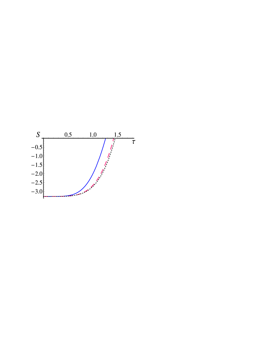
Figure 1: (Colors online) Separability function $S$ vs scaled time $\tau=\omega_{c}t$ with $r=1$ and $x_{1}=1$. The three curves are relative to different values of $x_{2}$. The blue solid line correspond to $x_{2}=1$, the red dashed line to $x_{2}=10$ and the black dotted line to $x_{2}=100$.

We start the analysis considering the case $x_{1},x_{2}\geq 1$. We show the entanglement evolution in Fig. 1 where we fixed the squeezing parameter to the value $r=1$. In this regime the dynamics is characterized by entanglement sudden death (ESD) appearing already in the short time non-Markovian region for any value of $r$. We also fixed the value of the parameter $x_{1}=1$ and plotted three curves correspondent to $x_{2}=1$ (solid blue), $x_{2}=10$ (dashed red) and $x_{2}=100$ (dotted black). We observe that the disentanglement time $\tau_{dis}$, defined as $S(\tau_{dis})=0$, only slightly increases as the adimensional frequency detuning $\Delta x=|x_{1}-x_{2}|$ increases.

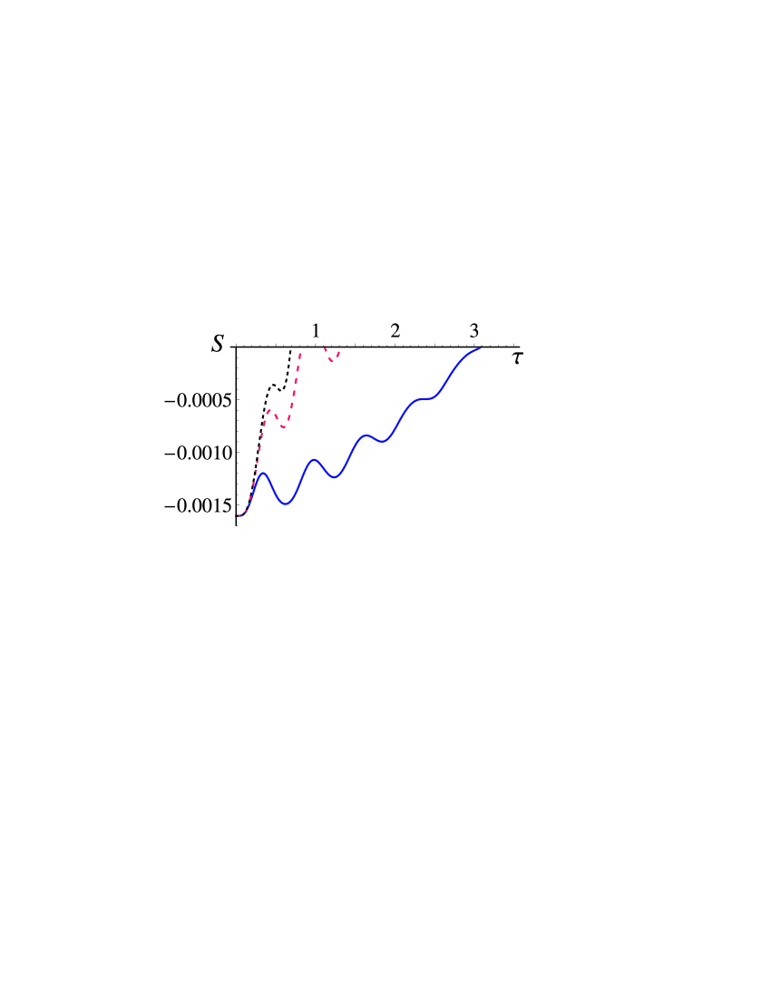
Figure 2: (Colors online) Separability function $S$ vs scaled time $\tau=\omega_{c}t$ with $r=0.04$ and $x_{1}=0.1$. The three curves are relative to different values of $x_{2}$. The blue solid line correspond to $x_{2}=0.1$, the red dashed line to $x_{2}=0.2$ and the black dotted line to $x_{2}=0.3$.

The case $x_{1},x_{2}<<1$ is reported in Fig. 2. As emphasized in detail in [1], this regime is characterized by a more variegate entanglement dynamics, showing oscillations, ESD and revivals. We report the situation relative to an initially small amount of entanglement correspondent to $r=0.04$ and $x_{1}=0.1$. The three curves correspond to $x_{2}=0.1$ (solid blue), $x_{2}=0.2$ (dashed red) and $x_{2}=0.3$ (dotted black). In all cases there are entanglement oscillations and ESD, while an entanglement revival is also present when $x_{2}=0.2$. As in the previous regime of Fig. 1 we notice that disentanglement time is larger when $\Delta x$ increases with fixed value of $x_{1}$. However here the differences in the disentanglement time are much more evident. Also oscillations are damped out as the detuning increases.

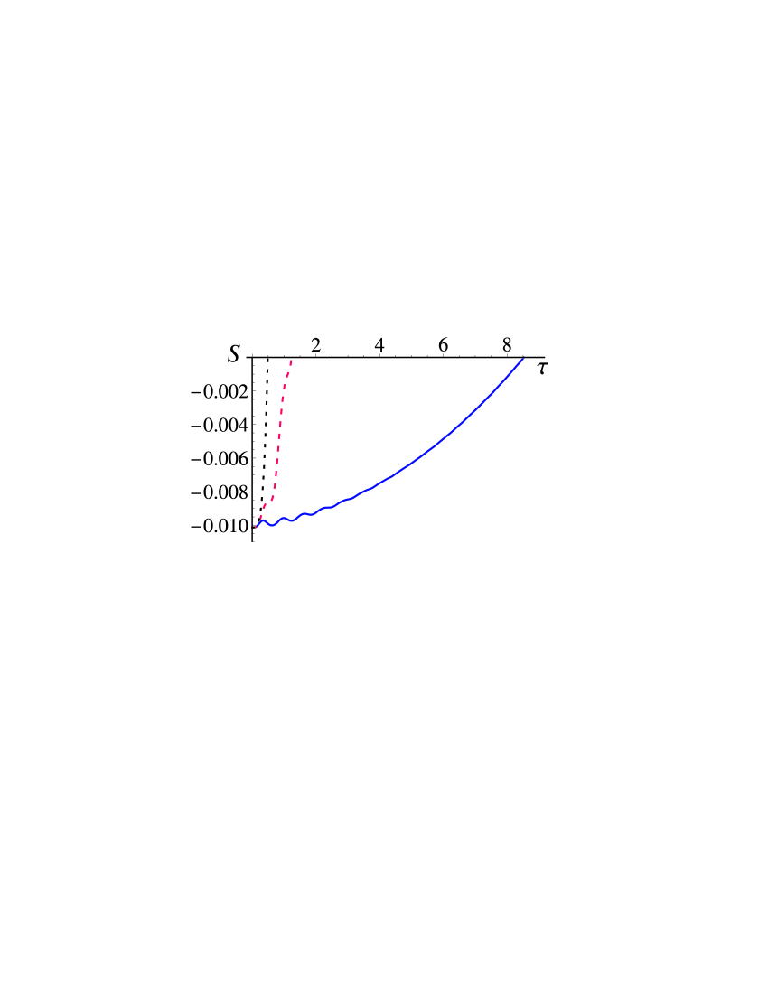
Figure 3: (Colors online) Separability function $S$ vs scaled time $\tau=\omega_{c}t$ with $r=0.1$. Blue solid line correspond to the choice $x_{1}=x_{2}=0.1$, red dashed line to $x_{1}=0.1,x_{2}=1$, and black dotted line to $x_{1}=x_{2}=1$

Finally we look at the regime $x_{1}<<1$ and $x_{2}\geq 1$ whose results are shown in Fig. 3 with the choice $r=0.1$. The blue solid line corresponds to $x_{1}=x_{2}=0.1$, the dotted black line describes the $x_{1}=x_{2}=1$ case, and the red dashed line represents the intermediate case of $x_{1}=0.1$ and $x_{2}=1$. Here we can observe two completely different behaviors of $S(\tau)$ relative to the cases $x_{1}=x_{2}=0.1$ and $x_{1}=x_{2}=1$. The former case is characterized by evident entanglement oscillations and a much longer survival time of entanglement. Instead the latter case shows a fast ESD without signs of oscillations. The intermediate case of $x_{1}\neq x_{2}$ possesses intermediate features: weak oscillations and a fast ESD.

The three parameters regimes analyzed display all the possible features in the entanglement dynamics for our particular system: entanglement oscillations, ESD and revivals. Thus when the oscillators frequencies are detuned no new qualitative behavior emerges, compared to the equal frequency case [1]. On the other hand we stress the existence of evident and non-negligible differences. This does not happen in the regime $x_{1},x_{2}>1$, where the value of disentanglement time increases only slightly as the oscillator detuning $\Delta x$ increases.

Quantitative differences characterize the opposite case, i.e., the regime $x_{1},x_{2}<<1$. Even a slight detuning ($\Delta x=0.1$) can change drastically the value of the disentanglement time and damp entanglement oscillations. Again this feature is present in Fig. 3 where these discrepancies are even more pronounced.

From our investigation we can extract two main results. When the oscillators have different frequencies ($\omega_{1}\neq\omega_{2}$), the entanglement dynamics shows a behavior which is intermediate between the cases of frequencies both equal to $\omega_{1}$ and both equal to $\omega_{2}$. Moreover the leading role in the disentanglement process seems to be played by the oscillator with higher resonance parameter $x$, which forces the entanglement to evolve in a way similar to the case of both parameters equal to the larger between the two, as shown in Fig. 3.

5 Summary

In this paper we extended the results obtained in [1] to the case in which the two oscillators have different free frequencies, thus when they interact with different parts of the reservoirs spectra. We considered the particular case of an Ohmic distribution in the high temperature limit for different initial TWB states and different values of the free oscillator frequencies. Quantitative differences in the entanglement dynamics can be observed in particular when both resonance parameters are in the regime $x<<1$, where the evolution changes also for a small values of $\Delta x$. On the contrary the dynamics is not strongly affected in the opposite regime even for large detuning. Moreover when the two frequencies lay in opposite parameters regime, the dynamics is similar to the case $x>>1$, characterized by lack of oscillations and fast ESD.

References

References

- [1] Vasile R, Olivares S, Paris M G A and Maniscalco S 2009 Phys. Rev. A 80 062324
- [2] Nielsen M A and Chuang I L 2000 Quantum Computation and Quantum Information (Cambridge: Cambridge University Press)
- [3] Weiss U 1999 Quantum Dissipative Systems (Singapore: World Scientific Publishing)
- [4] Braunstein S L and van Loock P 2005 Rev. Mod. Phys. 77 513
- [5] Prauzner-Bechcicki J S 2004 J. Phys. A 37 L173
- [6] Xiang S-H, Shao B and Song K-H 2008 Phys. Rev. A 78 052313
- [7] Serafini A, Illuminati F, Paris M G A and De Siena S 2004 Phys. Rev. A 69 022318
- [8] Dodd P J , Halliwell J J 2008 Phys. Rev. A 69 052105
- [9] Dodd P J 2008 Phys. Rev. A 69 052106
- [10] Hiroshima T 2001 Phys. Rev. A 63 022305
- [11] Maniscalco S, Olivares S and Paris M G A 2007 Phys. Rev. A 75 062119
- [12] Hu B L, Paz J P and Zhang Y 1992 Phys. Rev. D 45 2843
- [13] Simon R 2000 Phys. Rev. Lett. 84 2726
- [14] Intravaia F., Maniscalco S. and Messina A. 2003 Phys. Rev. A 67 042108