Current Modulator based on Topological Insulator
with Sliding Magnetic Superlattice

Abstract

We study theoretically the surface of a topological insulator with a sliding magnetic superlattice coated above. By analyzing time-dependent Dirac equations, the dynamics of the zero mode is investigated. When the superlattice’s sliding velocity is smaller (larger) than the Fermi velocity of topological insulator, the zero mode is perfectly (imperfectly) pumped. We also propose the application of this setup, which rectifies currents or generates pulse currents. It would provide a prototype of electronic devices based on topological insulator.

Introduction: Topological insulatorKane ; Bernevig ; Hsieh ; Today is a new state of matter with insulating bulk and metallic surface. The gapless surface is protected by the topology, and persisting even in the presence of disorder as long as time reversal symmetry is respected. Both theory and experiment have established that this surface is not a conventional metal, but a helical liquid. As a result, a dissipationless spin current can be realized on the surface.

When time reversal symmetry is broken on the surface, even richer properties of topological insulator emerges, such as monopolesZang and chiral Majorana fermionsMajorana . When a magnetic domain wall is attached on the surface, a chiral mode is generated inside the wall, which shares the same physics as Jackiw and Rebbi’s zero modeJackiw . In this sense, topological insulator bridges between condensed matter physics and high energy physics. Many unrealized phenomenon in high energy physics are promisingly addressed experimentally in topological insulator.

However, potential applications of topological insulator are seldom mentioned. Let us consider a magnetic domain-wall lattice created on its surface. Then, domain walls generate series of chiral zero modes, which are treated as quantum wires. By the motion of these domains, we can tune the electronic signals. It would provide a prototype of application in electronics.

In this paper, we find a dissipationless transverse current induced by a magnetic superlattice attached onto a topological insulator by solving time-dependent Dirac equations. The behavior changes drastically whether the sliding velocity of the superlattice is larger or smaller than the velocity of the Dirac particle. The transverse current is perfectly pumped when we apply a slowly moving magnetic lattice (adiabatic quantum pumping) and imperfectly pumped when we apply a fast moving lattice (non-adiabatic quantum pumping). We also suggest an application of this set up to a current modulator, which converts between direct, alternating, and repulse currents.

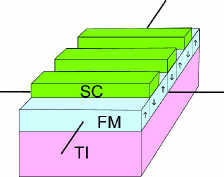
Figure 1: Illustration of an experimental setup of current modulator on the surface of a topological intulator.

Model: Our system consists of a three-dimensional topological insulator with a ferromagnet attached onto it [Fig.1]. Electrons obey 2D Dirac equations on the surface of a topological insulator, as has been demonstrated by the spin- and angle-resolved photoemission spectroscopyHsiehN . In the presence of a ferromagnetic layer on top of a topological insulator, the Hamiltonian is given by

$$H=\hbar v_{\text{F}}(k_{x}\sigma_{x}+k_{y}\sigma_{y})+\mu_{B}\mathbf{M}\left(\mathbf{x},t\right)\cdot\mathbf{\sigma},$$ (1)

where $v_{\text{F}}$ is the Fermi velocity of Dirac fermions, which is $3\times 10^{5}$m/s for Bi₂Se₃Zhang , $\sigma_{i}$ are the Pauli matrices, $\mu_{B}$ is the Bohr magneton, and $\mathbf{M}\left(\mathbf{x},t\right)$ represents the strength of the exchange coupling. It has been arguedYokoyama that the in-plane magnetic field contributes only tiny effects to the transport property of a topological insulator. Namely, it is a good approximation that $\mathbf{M}\left(\mathbf{x},t\right)$ has only the $z$-component, $\mathbf{M}\left(\mathbf{x},t\right)=\left(0,0,M\left(x,t\right)\right)$. Let us assume that the system is homogeneous along the $y$-axis. Then, the central point is the $x$ and $t$ dependence of this exchange coupling, which is realized by domain wall motion along the $x$-axis with velocity $v$ in the ferromagnet layer. It is reasonable to set

$$M\left(x,t\right)=m\sin\left[\left(x-vt\right)/\lambda\right]$$ (2)

to describe a domain-wall lattice, where $m$ is a numerical constant characterizing the strength of a single domain. We define $\omega=v/\lambda$.

Static solution: The sinusoidal behavior of $M(x,t)$ leads to a series of zero-field points periodically. As particle-hole symmetry is respected, according to Jackiw and Rebbi’s work, zero modes appear around these points. In order to derive the explicit expression of the zero modes here, let’s start from the time-dependent Schrödinger equation

$$i\hbar\partial_{t}\Psi=H\Psi,$$ (3)

where we have set the wave function as $\Psi=\left(\psi_{\uparrow},\psi_{\downarrow}\right)^{t}$. We may set $k_{y}=$constant in (1) due to the translational invariance along the $y$-axis.

We first study the static case where $\omega=0$. Particle-hole symmetry guarantees the existence of zero-energy solutions with the relation $\psi\equiv\psi_{\uparrow}=\pm i\psi_{\downarrow}$. When $k_{y}=0$, the equation of motion is transformed into

$$\mu_{B}M\left(x\right)\psi=\pm\hbar v_{\text{F}}\partial_{x}\psi.$$ (4)

We may solve it asJackiw

$$\psi_{\pm}\left(x\right)=\exp\left[\pm\frac{\mu_{B}}{\hbar v_{\text{F}}}\int_{0}^{x}M\left(x^{\prime}\right)dx^{\prime}\right],$$ (5)

which yields

$$\psi_{\pm}\left(x\right)=\exp\left[\pm\frac{\mu_{B}m\lambda}{\hbar v_{\text{F}}}\cos\frac{x}{\lambda}\right],$$ (6)

up to a normalization constant. We illustrate the magnetization and $\left|\psi\left(x\right)\right|^{2}$ for these two cases in Fig.2.

We may also present solutions for the non-zero $k$ case. The two solutions have opposite chirality, so their group velocity along $y$-direction is opposite as well. The wave function is a linear combination of $\psi_{\pm}\left(x\right)$,

$$\Psi=e^{ik_{y}y}\Psi_{+}+e^{-ik_{y}y}\Psi_{-},$$ (7)

with (6).

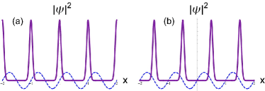
Figure 2: We illustrate the magenetization due to the magnetic superlattice $M\left(x\right)$ (dashed curve) and the static solutions $\left|\psi\left(x\right)\right|^{2}$ associated with it (solid curve), (a) for the $+$ sign and (b) for the $-$ sign in (6). The horizontal line represents the $x$ axis. We have set $\mu_{B}m\lambda/(\hbar v_{\text{F}})=5$.

Moving Domain Wall: We start with the investigation of the domain wall motion described by (2). The sinusoidal potential has a double-periodicity,

$$M\left(x+L,t\right)=M\left(x,t\right),\quad M\left(x,t+T\right)=M\left(x,t\right),$$ (8)

where $L=2\pi\lambda$ and $T=2\pi\lambda/v$. To such a system both the Bloch theorem and the Floquet theorem are applicable: The wave function is of the form $\psi_{\alpha}\left(x,t\right)=e^{i\varepsilon_{\alpha}t+ik_{\alpha}x}u_{\alpha}\left(x,t\right)$ with $u_{\alpha}\left(x+L,t\right)=u_{\alpha}\left(x,t\right)$ and $u_{\alpha}\left(x,t\right)=u_{\alpha}\left(x,t+T\right)$. Then it is enough to analyze the torus region $0\leq x<L,0\leq t<T$.

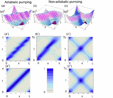
Figure 3: We show numerical solutions of the time-dependent Dirac equation with the sinusoidal potential for (a,a’) $\omega/\omega_{\text{c}}=0.25$, (b,b’) $\omega/\omega_{\text{c}}=3$, (c,c’) $\omega/\omega_{\text{c}}=10$. The vertical axis is $\left|\psi\left(x,t\right)\right|^{2}$. The horizontal axes are $x$ and $t$. (a), (b) and (c) are bird’s eye view and (a’), (b’) and (c’) are their contour plot. We also present analytic solutions in (a") and (c"), which are valid $\omega/\omega_{\text{c}}\ll 1$ and $\omega/\omega_{\text{c}}\gg 1$, respectively. The figures are plotted in the region $0<x<L,0<t<T$ for the adiabatic case, and in the region $0<x<L,0<t<T_{\text{c}}$ for the non-adiabatic case, where $T_{\text{c}}=(\omega/\omega_{\text{c}})T$. We have started from the static solution with $\mu_{B}m\lambda/(\hbar v_{\text{F}})=1$.

First we investigate the case where the velocity of the moving lattice is low, $v<v_{\text{F}}$, or $\omega<\omega_{\text{c}}$ with $\omega_{\text{c}}=v_{\text{F}}/\lambda$. We have carried out a numerical analysis of the time-dependent Dirac equation, starting from a static solution, whose results we give in Fig.3(a,a’), where we have set $\omega/\omega_{\text{c}}=0.25$. We find that the zero mode moves together with the magnetic lattice, and it is adiabatically pumped.

It is possible to derive the analytic solution based on the adiabatic approximation,

$$\psi_{\pm}\left(x,t\right)=\exp\left[\pm\frac{\mu_{B}m\lambda}{\hbar v_{\text{F}}}\cos\frac{\left(x-vt\right)}{\lambda}\right],$$ (9)

which is constructed by making the Galilei boost of the static solution (5): See Fig.3(a"). This solution is valid when the velocity is very low. There are fluctuations in $\left|\psi\left(x,t\right)\right|$ in the case of the numerical calculation, which is absent in the analytic one. This is because the adiabatic solution (9) is not an exact solution of (3). In any case, if we introduce the function $P_{n}(t)$ representing the position of $\left|\psi\left(x,t\right)\right|$’s n-th peak at time $t$ in unit of $\lambda$, we have

$$P_{n}\left(T\right)-P_{n}\left(0\right)=1$$ (10)

for $\omega<\omega_{\text{c}}$. In that sense, the zero mode is adiabatically pumped along $x$-direction as long as the velocity of domain wall motion is smaller than the Fermi velocity. As the Fermi velocity for topological insulator is generally very large, this requirement is usually satisfied. Due to the periodicity along $x$-direction, $P_{n}(t)$ actually doesn’t depend on $n\,$, and the subscript is neglected in the following.

It’s also interesting to investigate the case where the velocity of the moving lattice is fast, $v>v_{\text{F}}$, or $\omega>\omega_{\text{c}}$. We have carried out a numerical analysis, whose results we give in Fig.3(b,b’) and (c,c’), where we have set $\omega/\omega_{\text{c}}=3$ and $10$. Fig.3(b,b’) are plotted in the region $0<t<T$, while Fig.3(c,c’) are plotted in the region $0<t<T_{\text{c}}$ with $T_{\text{c}}=(\omega/\omega_{\text{c}})T$.

In the large $\omega$ limit, we give also an analytic solution. Since the magnetization oscillates very quickly, we can approximate the system by the one-period time-averaged equation of motionMCloskey ,

$$i\hbar\partial_{t}\psi=\overline{H}\psi,$$ (11)

where

$$\overline{H}=\frac{1}{T}\int_{0}^{T}H\left(x,t\right)dt.$$ (12)

The equation of motion is rewritten as

$$i\hbar\partial_{t}\psi=-i\hbar v_{\text{F}}\left(\partial_{x}\sigma_{x}+\partial_{y}\sigma_{y}\right)\psi,$$ (13)

or

$$\partial_{t}^{2}\psi=v_{\text{F}}^{2}\left(\partial_{x}^{2}+\partial_{y}^{2}\right)\psi.$$ (14)

It does not depend on $\omega$. The solution is given by $\left[\psi\left(x-v_{\text{F}}t\right)+\psi\left(x+v_{\text{F}}t\right)\right]/2$ with (6), which we display in Fig.3(c"). The agreement is good between the analytic and numerical solutions when the velocity is large ($\omega/\omega_{\text{c}}>10$).

The pumping rate is independent of $\omega$. It implies that one transverse current is pumped in the period which is not $T$ but $T_{\text{c}}$,

$$P\left(T_{\text{c}}\right)-P\left(0\right)=1.$$ (15)

The primitive torus $0<t<T$ has been extended to $0<t<T_{\text{c}}$. As a result, the pumping transverse current in one period $T$ is anti-proportional to the frequency,

$$P\left(T\right)-P\left(0\right)=\omega_{\text{c}}/\omega.$$ (16)

The reason of this imperfect pumping is that the transverse current can not follow the magnetic lattice because it moves too fast.

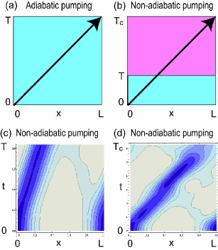
Figure 4: Schematic diagram of the adiabatic (a) and non-adiabatic (b) pumping. One transverse current is pumped in the time $T$ in the adiabatic pumping, while one transverse current is pumped in the time $T_{\text{c}}$ in the non-adiabatic pumping. Numerical results for the non-adiabatic pumping for the period (c) $[0,T]$, and (d) $[0,T_{\text{c}}]$.

A comment is in order. The adiabatic pumping case is experimentally realsitic, since it is hard to move domain walls faster than $v>v_{\text{F}}$ experimentally at this stage. Nevertheless the non-adiabatic case is theoritically very interesting, as we have shown.

In order to analyze the transition between the adiabatic and non-adiabatic pumpings, we calculate the pumping transverse current numerically. The pumping rate is estimated from the velocity of the position where $\left|\psi_{\uparrow}\left(x,t\right)\right|$ takes the maximum value at $t=T$. We show the numerical solution in Fig.5. It is seen that the pumping transverse current is well described by

$$P\left(T\right)-P\left(0\right)=\left\{\begin{array}[c]{ccc}1&\text{for}&\omega<\omega_{\text{c}}\\ \omega_{\text{c}}/\omega&\text{for}&\omega\gg\omega_{\text{c}}\end{array}\right..$$ (17)

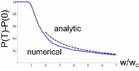
Figure 5: $\omega$ dependence of $P\left(T\right)-P\left(0\right)$. The horizontal axis is $\omega$ and the vertical axis is $P\left(T\right)-P\left(0\right).$

The analytic and numerical solutions show a good agreement. The change between the adiabatic and non-adiabatic transverse current pumping takes place rather suddenly. It may be a kind of a non-equiribrium phase transition.

Experimental setup: The realization of magnetic superlattice is a highly nontrivial question. Here we present an experimental proposal designed in the adiabatic pumping regime, as illustrated in Fig.1. On top of a topological insulator, a ferromagnetic thin layer is coated. Above the ferromagnetic layer, an array of periodically distributed superconductors is deposited. Usually there are many domains in the ferromagnet, which are naturally generated and hard to control. However, with the help of this array of superconductors, it becomes possible. At the beginning, an upward external magnetic field magnetizes the whole ferromagnetic layer in the same direction. Then, we lower the temperature below the critical temperature of superconductor, and reverse the direction of external magnetic field. Due to the Meissner effect, magnetic field is screened just below the superconductor, and unscreened elsewhere. As a result, magnetization in the areas without superconductor above is reversed, and the magnetization below the superconductor may remain unchanged if the external magnetic field is properly controlled. We would obtain a magnetic superlattice on top of a topological insulator in this way.

It is well knownYamaguchi that a current can drive the magnetic motion of domain walls. By introducing a current in the ferromagnetic layer along the $x$-direction, we can approximately realize the moving magnetic configuration in (2), and conducting channels provided by the zero modes are generated. Once the device is bridged by a conducting channel, a significant current is detected.

It’s an interesting property that the two zero modes in one period of the magnetic superlattice have opposite chiralities. These two conducting channels have tendency to transport opposite currents. We propose three type devices.

(a) When we do not apply the current into the ferromagnet, the magnetic superlattice is static. We apply an alternating voltage between two leads parallel to the domain wall. The resulting current is rectified into a direct current,

$$J_{\text{out}}=\max\left[J_{\text{in}},0\right],$$ (18)

because the zero-energy conducting channel is chiral and hence only the forward bias current goes through. This system rectifies alternating currents to direct currents, or acts as a diode.

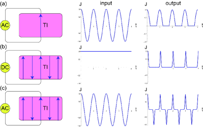
Figure 6: We show the time dependence of transverse current. (a) current rectifier (b) pulse generator (c) alternating pulse generator. We have set $\mu_{B}m\lambda/(\hbar v_{\text{F}})=10$.

(b) When we apply the current into the ferromagnet, the domain wall movesYamaguchi . We apply the direct voltage between two leads. The resulting current is modulated to be a pulse-current,

$$J_{+}\left(t\right)= \operatorname{Re}\left[\frac{\hbar}{2mi}\Psi_{+}^{\dagger}\partial_{y}\Psi_{+}\right]$$

$$= \frac{\hbar k_{y}}{2m}\exp\left[2\frac{\mu_{B}m\lambda}{\hbar v_{\text{F}}}\cos\frac{\left(x-vt\right)}{\lambda}\right],$$ (19)

because the zero energy conducting channel passes through the contact periodically according to the motion of domain walls. This system acts as a pulse generator.

(c) When we apply an alternating voltage to the same setup with (b), the resulting signal between two devices is an alternating pulse. This current is given by

$$J\left(t\right)= \operatorname{Re}\left[\frac{\hbar}{2mi}\Psi^{\dagger}\partial_{y}\Psi\right]$$

$$= \frac{\hbar k_{y}}{m}\sinh\left[2\frac{\mu_{B}m\lambda}{\hbar v_{\text{F}}}\cos\frac{\left(x-vt\right)}{\lambda}\right],$$ (20)

and is shown in Fig.6. This system acts as an alternating pulse generator.

It will be possible to measure these currents by attaching leads to the topological insulator parallel to the domain wall as in Fig.1.

Conclusion: In this paper, we have studied the dynamics of the zero mode in the presence of a magnetic superlattice on top of a topological insulator, which is described by a time-dependent Dirac equation. The domain wall motion of the superlattice is studied. We have proposed a prototype of electronic device based on the this theoretical studies, where the input current is found to be significantly modulated by the magnetic superlattice [Fig.1]. We hope this work can promote the application of topological insulator in future.

This work was supported in part by Grants-in-Aid for Scientific Research from the Ministry of Education, Science, Sports and Culture No. 20940011.

References

- (1) C.L. Kane and E.J. Mele, Phys. Rev. Lett. 95, 146802 (2005): ibid, 95, 226801 (2005).
- (2) B.A. Bernevig, T.L. Hughes and S.-C. Zhang, Science 314, 1757 (2006); X.-L. Qi, T.L. Hughes, and S.-C. Zhang, Phys. Rev. B 78, 195424 (2008).
- (3) D. Hsieh et al., Nature 452, 970 (2008). Y. Xia et al., Nat. Phys. 5, 398 (2009).
- (4) X.-L. Qi, S.-C. Zhang, Physics Today, 63, 33 (2010).
- (5) X.-L. Qi, R. Li, J. Zang and S.-C. Zhang, Science 323, 1184 (2009).
- (6) L. Fu and C.L. Kane, Phys. Rev. Lett. 100, 096407 (2008).
- (7) R. Jackiw and C. Rebbi, Phys. Rev. D 13, 3398 (1976).
- (8) D. Hsieh et al., Nature 323, 919 (2008). A. Nishide et al. cond-mat/arXiv:0902.2251.
- (9) Y. Zhang, et.al, cond-mat/arXiv:0911.3706.
- (10) T. Yokoyama, Y. Tanaka, and N. Nagaosa, cond-mat/0907.2810.
- (11) L. Fu and C.L. Kane, Phys. Rev. B 74, 195312 (2006).
- (12) X.-L. Qi, T.L. Hughes and S.-C. Zhang, Nature Physics 4, 273 (2008).
- (13) A. Yamaguchi, et.al, Phys. Rev. Lett. 92, 077205 (2004).
- (14) R.T. M’Closkey, Systems & Control Letters 32 179 (1997).