Observational Study of the Multistructured Planetary Nebula NGC 7354

Abstract

We present an observational study of the planetary nebula (PN) NGC 7354 consisting of narrow band H$\alpha$ and [N II]$\lambda 6584$ imaging as well as low and high dispersion long-slit spectroscopy and VLA-D radio continuum. According to our imaging and spectroscopic data, NGC 7354 has four main structures: a quite round outer shell and an elliptical inner shell, a collection of low-excitation bright knots roughly concentrated on the equatorial region of the nebula and two asymmetrical jet-like features, not aligned neither with the shells axes, nor with each other. We have obtained physical parameters like electron temperature and electron density as well as ionic and elemental abundances for these different structures. Electron temperature and electron density slightly vary throughout the nebula going from $\simeq 11,000$ to $\simeq 14,000$ K, and from $\simeq 1000$ to $\simeq 3000$ cm^-3, respectively. The local extinction coefficient $c_{{\rm H}\beta}$ shows an increasing gradient from South to North and a decreasing gradient from East to West consistent with the number of equatorial bright knots present in each direction. Abundance values show slight internal variations but most of them are within the estimated uncertainties. In general, abundance values are in good agreement with the ones expected for PNe. Radio continuum data are consistent with optically thin thermal emission. Mean physical parameters derived from the radio emission are electron density $n_{e}=710$ cm^-3 and $M$(H II)$=0.22\,M_{\odot}$.

We have used the interactive three-dimensional modeling tool shape to reproduce the observed morphokinematic structures in NGC 7354 with different geometrical components. Our observations and model show evidence that the outer shell is moving faster ($\simeq$ 35 km s^-1) than the inner one $\simeq$ 30 km s^-1. Our shape model includes several small spheres placed on the outer shell wall to reproduce to equatorial bright knots. Observed and modeled velocity for these spheres lies between the inner and outer shells velocity values. The two jet-like features were modeled as two thin cylinders moving at a radial velocity of $\simeq$ 60 km s^-1. In general, our shape model is in very good agreement with our imaging and spectroscopic observations. Finally, after modeling NGC 7354 with shape, we suggest a possible scenario for the formation of the nebula.

1 Introduction

Since the recognition that winds from the central stars of planetary nebulae (PNe) play an important role in the shaping of these objects (e.g. Kwok et al., 1978; Balick, 1987), and that only a small fraction of them show circular symmetry, the interest in PN morphology has triggered an active field in both theoretical and observational astronomy. Many studies have been devoted to classify (e.g., Balick, 1987; Schwarz et al., 1992; Manchado et al., 1996) and to model the basic morphologies observed (circular, elliptical and bipolar) with noticeable success (e.g., Balick et al., 1987; Hajian et al., 1997). However, high resolution images have shown that the morphologies of PNe are far from simple. Multiple shells, multipolar structures, highly collimated outflows, microstructures and peculiar geometries are present in many PNe and cannot be explained with simplistic models (e.g., Sahai & Trauger, 1998; Miranda et al., 2006; Miranda, Pereira & Guerrero, 2009). Nowadays, it is accepted that highly collimated outflows play a crucial role in the shaping of PNe (Sahai & Trauger, 1998). Nevertheless, other physical processes are probably present, so that most likely the shaping of PNe is a result of many processes acting at the same time (e.g., Balick & Frank, 2002). In order to understand complex PNe, the first step is to identify the structural components present and to define their nature. High-resolution, spatially resolved spectroscopy combined with narrow-band imaging has demonstrated to be a powerful tool to disentagle the structural components in PNe, to infer their nature and to constraint the ejection processes involved in their formation (Miranda & Solf, 1992; Vázquez et al., 1999, 2008; Guerrero et al., 2008; Vázquez et al., 1998; López et al., 2000).

Although at first glance NGC 7354 looks like an elliptical PN, extense H$\alpha$, [O III]$\lambda 5007$, [N II]$\lambda 6584$ and mid-infrared imaging and spectroscopic data have revealed that it possess a more complex structure (Sabbadin et al., 1983; Balick, 1987; Hajian et al., 1997; Phillips et al., 2009). In particular, Balick (1987) described this nebula as consisting of an inner halo, a thin bright rim, two spike-like tails, and low-excitation patches projected onto the rim-halo interface. The large-scale structures observed in NGC 7354 are qualitatively well described using the interacting winds theory (e.g. Balick et al., 1987; Mellema, 1995; Hajian et al., 2007) but no deep analysis has been carried out for the small-scale structures and their relationship with the large-scale ones.

In this work we present a detailed observational study of the morphology, internal kinematics, and physical and chemical properties of NGC 7354. These data allow us to discuss and model each of the components present in the object and to suggest a possible scenario for the formation of this nebula.

2 Observations and Results

2.1 Optical Imaging

Narrow-band images of NGC 7354 were obtained on 1997 July 24 with the Nordic Optical Telescope (NOT) and the HiRAC camera equiped with a Loral CDD of 2048$\times$2048 pixels and a plate scale of $0\hbox to0.0pt{.\hss}{{}^{\prime\prime}}11$ pixel^-1. Two narrow-band filters were used: [N II]$\lambda 6584$ ($\Delta\lambda=10$ Å) and H$\alpha$ ($\Delta\lambda=10$ Å). The exposure time for both filters was 900s. Seeing was about $0\hbox to0.0pt{.\hss}{{}^{\prime\prime}}9$ during the observations.

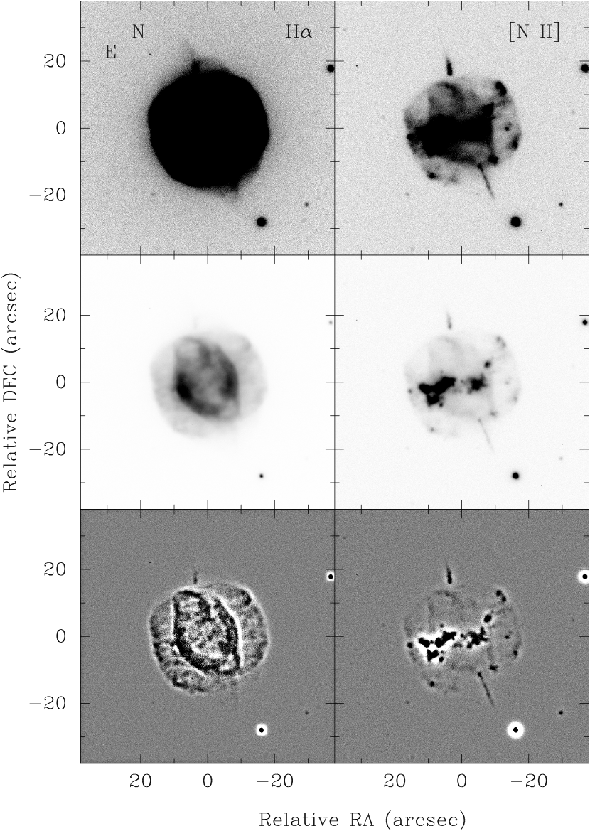
Figure 1: Grey-scale representations of the images of NGC 7354 in the light of H$\alpha$ (left panels) and [N II]$\lambda 6584$ (right panels). Two different contrasts have been used to show up the faint and bright nebular structures. Unsharped masking images are also present (lower row) in order to see details of the nebula.

Figure 1 shows a mosaic of our H$\alpha$ and [N II] images, including unsharp masking images in both filters constructed to show up both the large- and small-scale structures in the nebula. In these images, we can identify the main structures previously described by other authors: the outer shell, the elliptical inner shell, the bright equatorial knots, and the two jet-like features. In the following we will describe in more detail each of these structures as well as new morphological details that have not been previously mentioned.

The outer shell looks like a round envelope in the high-contrast images but it appears as a faint cylindrical structure in the low-contrast images. Its size is $\simeq 33^{\prime\prime}\times 29^{\prime\prime}$ with the major axis oriented at position angle PA $\simeq 15^{\circ}$. The outer shell is brighter in H$\alpha$ than in [N II] although in [N II] several bright knots are observed at the edges of it.

The inner shell present an elliptical shape with its major axis oriented at PA $\simeq 30^{\circ}$ and a major and minor axis length of $\simeq$ 21^′ $\times$ 16^′′, respectively. This structure is noticeable fainter in [N II] than in H$\alpha$. Moreover, the regions along the minor axis are particularly bright in H$\alpha$. A closer inspection of the images shows that the polar regions deviate from the elliptical shape and appear as two bubbles. This is particularly noticeable in H$\alpha$. We will refer to these regions of the inner shell as the polar caps .

The bright equatorial knots are observed in [N II] but not in H$\alpha$. They are mainly concentrated in two groups, East and West, and along the equatorial plane of the outer and inner shells.

The two jet-like features are bright in [N II] but much fainter in H$\alpha$. The northern feature is oriented at PA$\simeq 13^{\circ}$ and extends $\simeq 7^{\prime\prime}$. The southern feature is oriented at PA $\simeq 205^{\circ}$, extends $\simeq 11^{\prime\prime}$, and appears narrower than the northern one. We note that the orientation of these two features does not coincide with each other nor with the orientation of the outer and inner shells.

In order to improve the view of NGC 7354, we retrieved a Hubble Space Telescope (HST) image from the MAST Archive (Proposal ID: 7501; P.I.: A. Hajian; date of observation: 1998 July 21; filter F658N; exposure time 1000 sec). Fig. 2 shows this image. The morphology of the outer and inner shells is similar to that observed in ground based images (Fig. 1). The jet-like freatures appear as cometary tails with a bright knot facing the central star and faint tails directed outwards. They present a knotty structure, particularly the southern one. The HST image resolve the bright equatorial knots into a series of small knots and filaments embedded in diffuse emission.

2.2 Radio continuum

The $\lambda 3.6$ cm radio continuum observations were made with the Very Large Array (VLA) of the NRAO on 1996 May 31 in the DnC configuration. The standard VLA continuum mode with a bandwidth of 100 MHz and two circular polarizations was employed. Phase center was set at RA(2000.0)=22^h40^m20$\fs$1, DEC(2000.0)=+61°17′06$\farcs$0. Flux calibrator was 3C48 (adopted flux density 3.3 Jy) and phase calibrator was 0019+734 (observed flux density 1.0 Jy). Total on-source integration time was 30 minutes. The data were calibrated and processed using standard procedures of the Astronomical Image Processing System (AIPS) package of the NRAO.

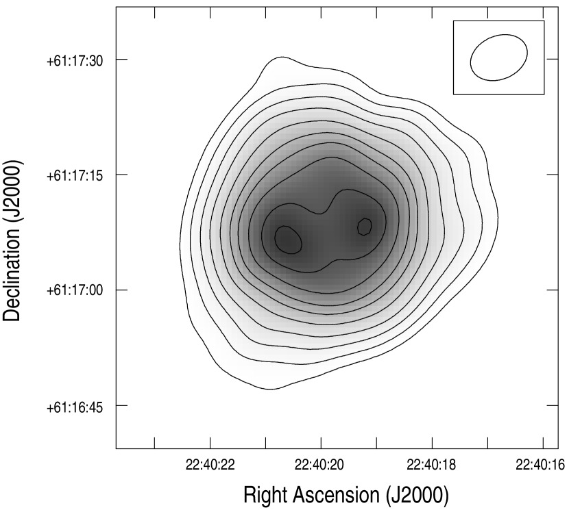
Figure 3: Grey-scale and contour uniform-weighted map of NGC 7354 at 3.6 cm radio continuum. Contour levels are 8, 18, 35, 60, 100, 150, 200, 270, 350, and 400 times 144 $\mu$Jy beam^-1, the rms noise in the map. The half-power beam width ($8\farcs 0\times 6\farcs 5$, PA $-86\arcdeg$) is shown in the upper right corner.

Fig. 3 shows an uniform-weighted map of NGC 7354. The emission presents a circular morphology and extends $\simeq$42″ in diameter. Two emission maxima are observed separated by $\simeq$10″ and oriented at PA$\simeq 100\arcdeg$. These emission maxima coincide with the H$\alpha$ bright regions observed along the minor axis of the inner shell.

From our data we derive a peak flux density of 72 mJy beam^-1 at position RA(2000.0)=22^h40^m20$\fs$44, DEC(2000.0)=+61°17′06$\farcs$8, and a total flux density of $502\pm 4$ mJy. We note that our map is similar to that obtained by Terzian et al. (1974), being the flux density values obtained in both works consistent with each other and with optically thin thermal emission. Adopting a distance of 1.5 kpc for the nebula (Sabbadin, 1986, see Sec. 3.1) and following the formulation by Mezger & Henderson (1967), we derive a mean electron density of $\simeq$ 710 cm^-3 and an ionized mass of $\simeq$ 0.22 $M_{\odot}$.

2.3 Low Resolution Spectroscopy

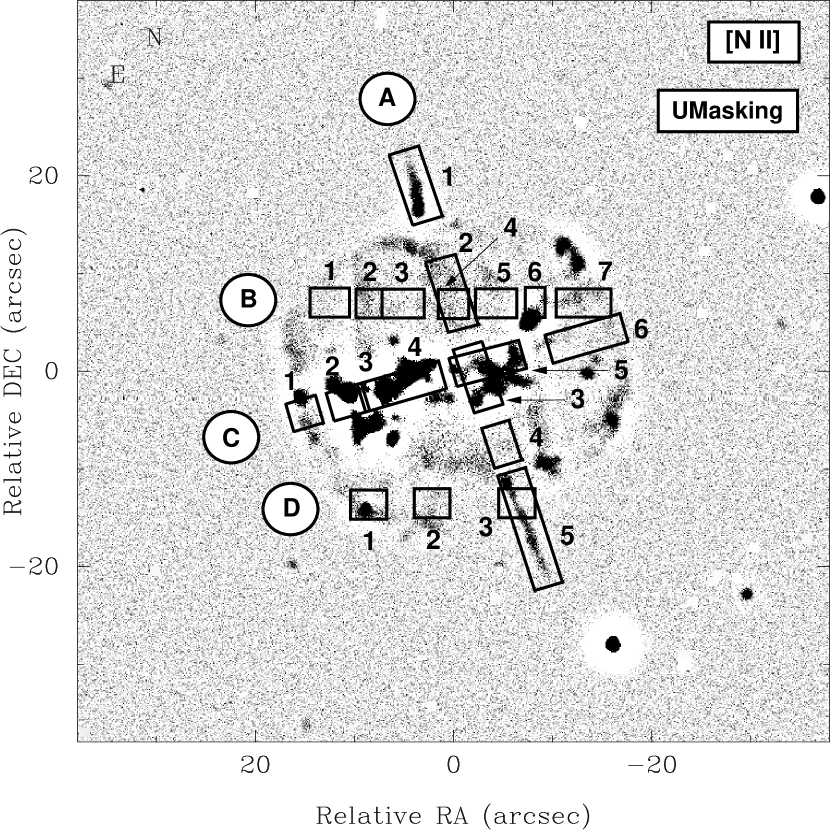
Figure 4: Slit positions (A,B,C,D) used for low resolution spectroscopy superimposed on the unsharped masking [N II]$\lambda 6584$ image. Along each slit position several regions (1,2,3,…) were selected to analyze specific structures of the nebula.

Low resolution, long-slit spectra were obtained with the Boller & Chivens spectrograph mounted on the 2.1 m telescope at the San Pedro Mártir Observatory (OAN-SPM) during three observing runs: 2002 June 14, 2002 August 7, and 2002 December 10 and 11. A CCD SITe with $1024\times 1024$ pixels was used as a detector. We have used a 400 lines/mm dispersion grating and a slit width of 2″ giving a spectral resolution (FWHM) of 7Å. Spectra reduction was performed using IRAF standard procedures. We have used four slit positions to cover specific regions of the nebula. Fig. 4 shows these slits, labelled A to D, and the regions extracted from each long-slit spectrum overplotted on the unsharp masking [N II] image. Regions are denoted by a letter refering to the slit position followed by a sequence number along the slit. In total, 21 regions in NGC 7354 have been analyzed.

Table 1 presents dereddened line fluxes, observed H$\beta$ flux and the logarithmic extinction coeficiente $c{{}_{\rm H\beta}}$ for each region, the last has been derived from the observed H$\alpha$/H$\beta$ ratio assuming case B recombination. The fluxes have been dereddened aplying the extinction law by Cardelli, Clayton & Mathis (1989). Electron temperature ($T_{e}$) has been derived from the [O III] and/or [N II] emission lines, while electron density ($N_{e}$) has been derived from the [S II], [Cl III] and/or [Ar IV] emission lines, in both cases using the Five-Level Atom Diagnostic Package NEBULAR (DeRobertis, Dufour & Hunt, 1987; Shaw & Dufour, 1994) from IRAF. Derived physical parameters and their estimated errors are shown in Table 3. Error estimates take into account the readout and photon noise and they are propagated along the calculation of physical quantities. Whenever possible, $N_{e}$ values were calculated using the value of $T_{e}$ derived from the corresponding high- or low-excitation ion, [O III] or [N II], respectively.

Extinction within the nebula, as indicated by $c_{\rm H\beta}$, shows a slight increase from South to North with values ranging from $\simeq$ 1.7 to $\simeq$ 2.4, respectively. Relatively high values of $c_{\rm H\beta}$ $\simeq$ 2.4 are found in the low-excitation equatorial knots. These values can be compared to those in the surroundings of the knots where the extinction decreases up to $c_{H\beta}$ $\simeq$ 1.7. This result suggests that the equatorial knots are denser and/or contain more dust than the rest of the nebula.

Electron density slightly increases inwards from the outer shell (regions B1 and C6) with values of $\simeq$ 1 000 cm^-3 to the inner regions of the inner shell (region B4) where values of $\simeq$ 2 400 cm^-3 are found. The bright equatorial knots are clearly denser that both the outer and inner shells with an average density of $\simeq$ 2 600 cm^-3. For the jet-like features, the electron density is relatively low with values around $\simeq$ 1 300 cm^-3.

Electron temperature also seems to slightly increase from $\simeq$ 13,000 K at the walls of the outer shell (regions B1, B6 and B7) to $\simeq$ 15,000 K at the center of the inner shell (region B3). In the bright equatorial knots, electron temperature ranges from $\simeq$ 10,000 to $\simeq$ 12,400 K. For the northern jet-like feature, no [O III] and [N II] lines were detected with a good signal-to-noise; in the southern jet-like feature, we have obtained an electron temperature of $\simeq$ 12,000 K (regions A5 and D3).

Ionic and elemental abundances values are listed in Tables 3 and 4, respectively. They have been obtained with the task IONIC in IRAF and using the ionization correction factors by Kingsburgh & Barlow (1994), respectively. Table 5 also lists abundances in other objects for comparison purposes. Small abundance variations, within the estimated uncertainties, are observed throughout NGC 7354. In general, we found that all our abundance determinations are consistent with those of PNe, see Table 5. Since neither He nor N overabundance is observed, as in the case of Type I PNe, we can say that it behaves like a Type II PN.

Elemental abundances for NGC 7354 have been reported by several authors (Hajian et al., 1997; Martins & Viegas, 2002; Perinotto et al., 2004a; Stanghellini et al., 2006). However, a comparison of our abundance estimations with those from the literature is not straightforward since we have obtained abundance values for several slit positions and specific regions along them. In the case of Hajian et al. (1997), they report abundance values of six regions along a slit position very similar to our slit A. Their abundances tend to be two or three times higher than ours in the case of O/H, N/H and S/H but lower in He/H and similar in Ar/H. Comparison with other studies can only be done through average values along each of our slit positions or the total average obtained from all our studied regions. We have compared our total averaged O/H, N/H, S/H, Ar/H abundances with those from Perinotto et al. (2004a) and Stanghellini et al. (2006). In both studies, their abundances seem to be lower than ours but in the case of Stanghellini et al. (2006) this difference may be due to tha fact that they consider the PN as a whole and excluded special features in the nebula.

2.4 High Resolution Spectroscopy

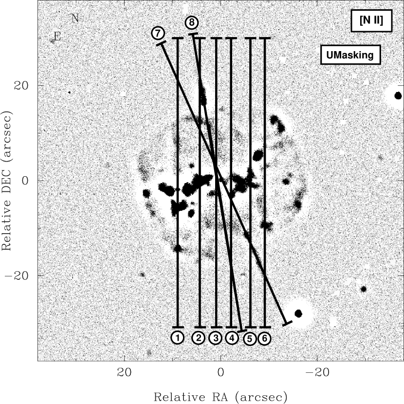
Figure 5: Slit positions used for high dispersion spectroscopy superimposed on the unsharped masking [N ii] image. The slits are numbered from 1 to 8. Slit numbers 7 and 8 are oriented at PAs 25°and 13°, respectively.

High-resolution, long-slit spectra were obtained in 2002 July 15 to 17 and 2007 July 10 to 17 with the Manchester Echelle Spectrometer (MES; (Meaburn et al., 2003)) mounted on the 2.1 m telescope at San Pedro Mártir Observatory (OAN-SPM). A Site CCD with 1024$\times$1024 pixels was used as a detector. Binnings of $1\times 1$ and $2\times 2$ were used in 2002 and 2007, respectively. Slit width was 1.6″  and the achieved spectral resolution (FWHM) is 12 km s^-1. The slit was oriented North-South and centered at several right ascensions across the nebula, except in those slits that covered the jet-like features, which have been centered on the central star and oriented at PAs 13^∘ and 25^∘. Figure 5 shows the used slit positions, numbered from 1 to 8, superimposed on the unsharp masking [N II] image. Data reduction was carried out with the IRAF package.

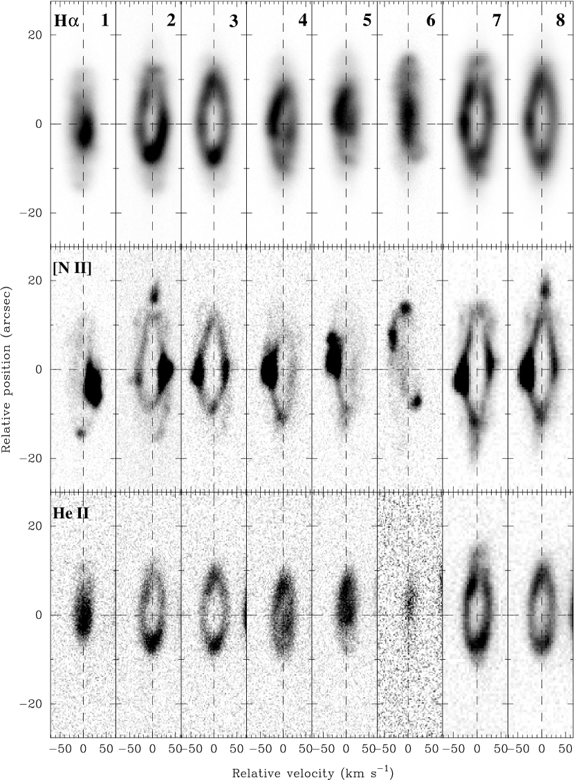
Figure 6: Grey-scale position-velocity maps of the H$\alpha$ (upper panels), [N II]$\lambda 6584$ (middle panels) and He II $\lambda 6560$ (lower panels) emission lines derived from the long-slit spectra at slit positions 1 to 8 (indicated in the H$\alpha$ panels for each column (see Fig. 5). The vertical and horizontal dashed lines in each panels indicate the systemic velocity of the nebula and the declination of the central star, respectively. North is up in each panel.

Grey-scale, position-velocity (PV) maps, derived from the eight long-slit spectra, are shown in Fig. 6 for the H$\alpha$, [N II]$\lambda 6584$, and He II$\lambda 6560$ emission lines. From the long-slit spectra, we derived a heliocentric systemic velocity of $-42\pm 2$ km s^-1 for NGC 7354, in excellent agreement with $-41\pm 2$ km s^-1 deduced by Sabbadin et al. (1983). Through this paper, we will consider the systemic velocity as the origin for quoting internal radial velocities and the declination of the central star as the origin for quoting distance measurements. The PV maps allow us to recognize the structural components that have been identified in the direct images. In the following, we will describe the spatio-kinematical properties of these components.

The [N ii] emission from the outer shell is recognizable at slit positions 1,2,3,5, and 6. The emission is very faint and in the central nebular regions it appears superposed by the stronger emission from the inner shell. Maximum radial velocity of $\simeq$ 35 km s^-1 is observed at the center and decreases with distance to the central star. Emission from the outer shell can be recognized in the H$\alpha$ line (Fig. 6) by its spatial extend. However, the large thermal width and, probably, low expansion velocity in this line do not allow us to obtain detailed kinematic information. The outer shell cannot be recognized in the long-slit spectra of the He II$\lambda 6560$ line.

The inner shell can be identified at all slit positions in the three lines. The emission feature of the inner shell appears as a velocity ellipse in the PV maps. The size of the velocity ellipse is maximum at slit 8 with values of 30^′′ in H$\alpha$ and [N II], and 20^′′ in He II. Maximum velocity splitting is observed at the center of the nebula (slits 3, 7, and 8) and amounts 60, 56 and 48 km s^-1 in H$\alpha$, [N II], and He II, respectively. This implies expansion velocities for the inner shell of 30, 28 and 24 km s^-1, respectively. Since we estimate an error of $\leq 1$ km s^-1 in our velocity measurements, these results show that the He II emission is confined to a slow expanding, inner thin layer of the inner shell while the [N II] traces the outer layer that expands faster.

It is worth noticing the very faint and wide emission observed in [N II] (slit positions 2, 3, 7 and 8) located at about 12″ and 8″ to the North and South of the central star, respectively. The velocity of this faint emission spreads from $\simeq-45$ to $\simeq 33$ km s^-1. Comparing our [N II] direct image and these particular PV maps, we identify these weak emissions with the two polar caps located on the main symmetry axis of the inner elliptical shell.

All slit positions in our [N II] PV maps, show the presence of at least one of the bright low-ionization knots identified in our optical [N II] images (Fig. 1, right panel). In all these PV maps we can see that most of them are located very close to the zero position line, i.e. almost on the equatorial plane of the nebula. Although these PV maps show that emission arising from different bright knots may be mixed due to projection effects, we can estimate that their expansion velocity ranges between the inner and outer shell expansion velocities, 28 km s^-1 to $\simeq$ 40 km s^-1, with only two of them having lower velocities, $\simeq$ 24 km s^-1. A final remark on the low-ionization knots is that in our [N II] PV maps, slit positions 1 and 6, we can see two weak spots of emission almost simetrically located at about 14″ to the North and South from the central star, respectively. Both emission spots show negative and very low velocities of $\simeq\,-5$ km s^-1. We identify these two spots of emission as coming from two bright knots that, in projection, appear to be located on the outer shell wall (see Fig. 1, [N II] images).

Although [N II] emission from the two jet-like features can be identified at slit positions 2 and 5 (Fig. 6), it can be better analyzed at slit positions 7 and 8 which were specially selected to cover these structures. In the corresponding PV maps we can see the conspicuous emission arising from the two jet-like features. While the North jet-like feature emission is slightly redshifted, the South feature is slightly blueshifted. Both features show a small radial velocity, between 0 and 5 km s^-1 which suggest that they are moving almost in the plane of the sky.

3 Discussion

3.1 Morphokinematic structure and modeling

As we have described, NGC 7354 shows four different structures: two large scale structures, the outer and the inner shells, the last having two polar caps located on its symmetry axis; a number of low-ionization bright knots lying about the equatorial plane, and two jet-like features located close to the North and South of the nebula, slightly inclined respect to the inner shell symmetry axis. Our high dispersion spectra indicate that (a) the inner shell is expanding with a velocity which is smaller than that of the outer shell, (b) most of the bright equatorial knots are moving at velocities closer to the outer shell, and (c) the jets’ projected velocity is very small.

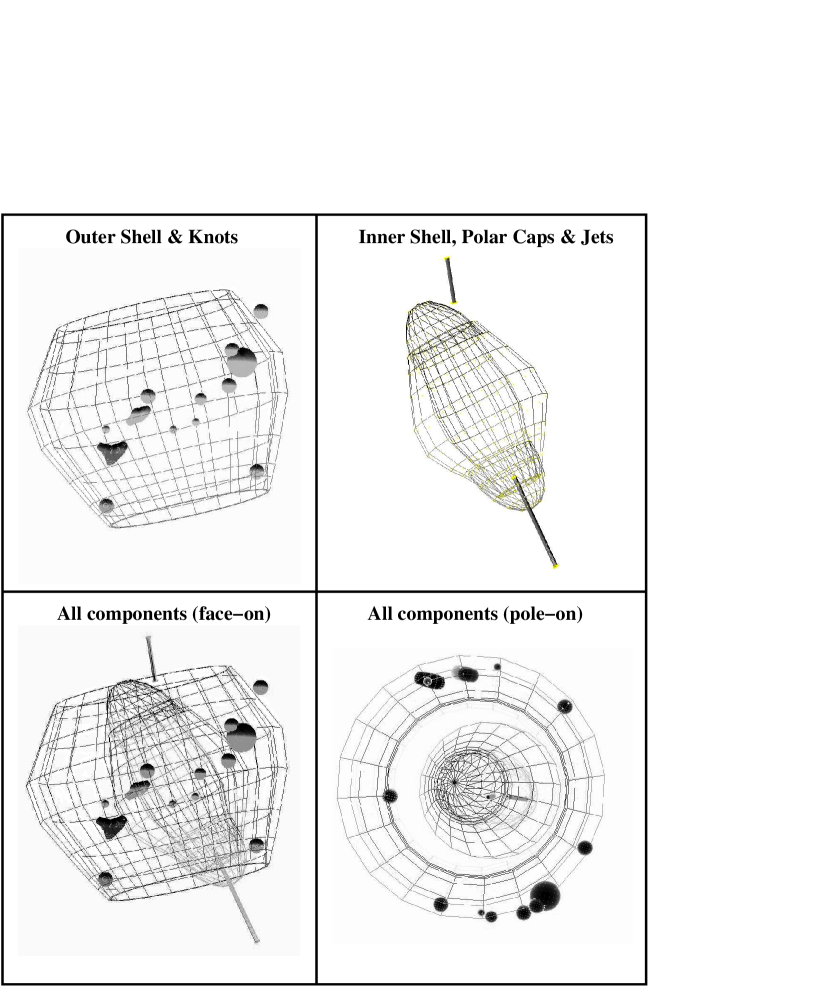
Figure 7: Upper panels show two sets of geometrical components used in the shape model. Lower panels show all components seen from two different angles, face-on (lower left panel) and pole-on (lower right panel).

In order to test the overall morphology and kinematic structure of the nebula we have used the interactive three-dimensional (3D) modeling tool shape Ver. 2.0 (Steffen & López, 2006). shape produces synthetic images and PV diagrams which can be compared directly with our observed CCD images and PV maps. We have considered two ellipsoidal structures (inner and outer shells), two spherical sections (polar caps), several small spheres with different diameter (bright knots) and two geometrically thin cylinders of 2^′′ in diameter (jet-like features). All these geometrical structures were slightly modified (smoothered, lengthened and/or rounded) in order to match the overall looking of our [N II] images. Besides, all the structures were placed on the proper position to get the corresponding observed radial velocity from our PV maps. Fig. 7 shows all the geometrical components used to construct our shape model.

Each one of the main structures was analized separately in order to obtain its spatial velocity independently. Due to projection effects we are unable to distinguish neither if the low-ionization knots are located between the inner and outer shell nor if they are lying on the foreground or on the background side of the nebula. Thus, we have assumed that the bright knots are located on the outer shell wall, according to their individual velocity shown in our PV map. It is important to remark that the inclination angle of the different structures is unknown and shape does not solve it. Final geometrical and kinematic parameters are shown in Table 6. Some of the inner shell basic parameters can be compared to those found by Hajian et al. (2007) with an extended prolate ellipsoidal shell model. While our derived inclination and position angles are consistent with the ones determined by Hajian et al. (2007), our expansion velocity value is larger than theirs. However, as they have found in all the cases examined in their study, the [N II] gas has a larger expansion velocity than the [O III] gas. Then, since we have determined the expansion velocity through the [N II] line emission, a difference in expansion velocities is expected. Distance estimations found in the literature lie around 1.2 kpc (Cahn et al., 1992; Zhang, 1995; Phillips, 2004) being 1.5 kpc the largest estimation (Sabbadin, 1986) and 0.88 kpc the smallest one (Daub, 1982). We have adopted the largest value of 1.5 kpc in order to derive an upper limit for the kinematical ages. However, using a distance value of 1.2 kpc implies a decrease in the kinematical age estimation of only 20%. But most important, distance uncertainty does not modify the proposed chronological sequence of structure formation in our model.

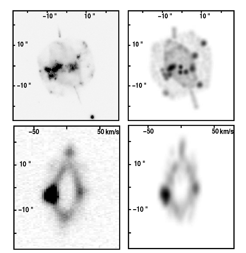
Figure 8: Comparison of observed data and the 3D model obtained from shape. Upper panels show the observed [N II] image (left panel) and the shape image (right panel). Lower panels show the observed PV map of the [N II]$\lambda 6584$ line at slit position 7 (left panel) and the corresponding shape synthetic PV map (right panel).

From this model, we have obtained synthetic images and PV diagrams which strongly resemble the observed ones, see Fig. 8 for an example of this good match. Thus, from the proposed 3D model we have not only reproduced qualitatively the overall morphology of NGC 7354 but we have also quantitatively reproduced the kinematic behaviour of each structure.

3.2 Formation of NGC 7354

At present, binary star models have been succesful in explaining the origin and process responsible for the equatorial density enhacement required in the interacting stellar wind (ISW) model, or rather the generalized ISW (GISW) model, to explain early- and middle-type elliptical and even bipolar large scale structures observed in PNe (e.g. Balick et al., 1987; Mellema, 1995; Mellema & Frank, 1995). On one hand, common envelope (CE) evolution in close binaries has been proposed to be responsible for the expanding slow wind torus needed in GISW (e.g Rasio & Livio, 1996; Frank et al., 1996; Terman & Taam, 1996; Sandquist et al., 1998). On the other hand, accretion disks in binary systems seem to account for the narrow waist bipolar morphologies and even the jets present in PNe. Details may vary on each binary model in order to explain individual morphologies and structures, but in all of them the main idea is that of a jet launched by the central star, or its companion (Soker & Rappaport, 2000; García-Arredondo & Frank, 2004; Sahai et al., 2007; Dennis et al., 2008; Akashi & Soker, 2008, among others).

Since at first glance NGC 7354 looks like a rather elliptical nebula, one may think that the single star models (ISW or GISW) can explain the presence of the outer and inner shells, and even the formation of the two jet-like features observed in our [N II] image (Balick et al., 1987). However, it is unable to explain why all the different structures show different position angles (PA’s) on the sky. This characteristic may indicate that the direction of ejection varies with time, and more likely that all the features were formed as independent events. Although nowadays there is no evidence of NGC 7354 possessing a binary nucleus, one may turn around and take a look at binary star models to try to understand in a consistent way the observed morphology of NGC 7354.

It has been proposed that the GISW model coupled with the predictions of the CE evolution theory can account for the formation of elliptical and even bipolar PNe morphologies (Soker & Livio, 1994). Then, we could succesfully explain the outer and inner shells in NGC 7354 based on this mixed model in the following way. After the CE phase has ended, i.e. the envelope has been ejected, the binary may become closer, mass transfer take place, an accretion disk is formed and a jet may be launched (Soker & Livio, 1994). If we assume that the subsequent evolution is similar to those described in the models for pPNe (Soker & Rappaport, 2000; Lee & Sahai, 2003; Dennis et al., 2008; Akashi & Soker, 2008) it is possible that a jet arise from an accretion disk. Then, the accretion disk theory would be able to explain also the two jet-like features observed in NGC 7354. Moreover, some of these models even propose the formation of an expanding dense ring in the equatorial plane (Soker & Rappaport, 2000) which in the case of NGC 7354 might be related to the equatorial bright knots. As the nebula evolve, a combination of the processes and mechanisms just mentioned might take place.

With this in mind, we suggest a possible qualitative scenario for the formation of the main structures present in NGC 7354. A slow wind is lost by a central binary system ongoing a CE phase, producing the mild elliptical outer shell. When the AGB fast wind begins, it finds an equatorial density enhaced enviroment forming the bright elliptical rim or inner shell. At this point the CE has been completely ejected and mass transfer from the secondary (main-sequence star) into the primary (white dwarf) will form an accretion disk and eventually a couple of jets will be launched. Once the jets have appeared, they will “push” the polar ends of the inner shell, detaching them from it. Eventually, the two jets would break the caps and escape from the main body of the nebula. Along with the processes mentioned, the binary system may be precessing and each of the structures would show a different PA on the sky. In the case of the two jets, precession may cause that they impinge on the polar caps with a certain angle, i.e. not along the symmetry axis of the caps, breaking them apparently on the “base” of them. According to our derived kinematical ages, the chronological sequence of formation seem to be consistent with the above description. The outer shell is the oldest structure present in the nebula with an age of about 2500 yr. The next younger structure would be the inner elliptical shell with $\simeq$1600 yr. Kinematical ages for the two jet-like features indicate that they are coeval and both were formed almost at the same time as the inner elliptical shell. However, we should notice that the age was derived assuming that they have been moving with the same velocity (60 km s^-1) since their launch. According with the theory of formation of jets this low initial velocity would be very unlikely, since they arise from accelerated flowing material. Then, more likely the jets possessed a higher initial velocity but they have been restrain along its way. Maybe the main cause of this decceleration was the interaction of the jets with the polar caps.

Regarding the equatorial low-excitation bright knots, as we have mentioned above they may be related to the dense expanding ring formed around the binary system. The bright knots show velocities ranging between the inner and outer shell expansion velocities. This may indicate that they are moving with a similar velocity as the particular ambient gas in which they are embedded. We may compare these bright knots with the microstructures observed in NGC 2392 (eskimo nebula, O’Dell et al., 2002) and NGC 7662 (Perinotto et al., 2004b). Although each one of these nebulae is seen with a different view angle (NGC 2392 is seen pole-on and NGC 7662 is seen edge-on) both of them show various low-ionization knots located beyond the inner structure and mainly on the outer envelope. If we compare the general morphology of NGC 7354 with that observed in NGC 2392 and NGC 7662 one can see that the three of them show an ellipsoidal inner structure surrounded by on outer envelope with low-ionization bright knots located on the outer structure plus jet-like features, interpreted as FLIERs in the case of NGC 7662. In the case of NGC 7354 since it is observed with an edge-on view angle and it is inclined with respect to the plane of the sky, we are not able to observe the real morphology of the equatorial brights knots. However, one can imagine that if one could get a pole-on view, i.e. with the inner shell major axis aligned with our line of sight, one would see bright knots located in a zone between the inner and outer shell very alike the arragement of knots with tails observed in the eskimo nebula. Therefore, having all these elements together, we suggest that, as in the cases of NGC 7662 and NGC 2392, the equatorial bright knots observed in NGC 7354 are not spherical structures but knots with tails, or even filamentary structures. This last suggestion is strongly supported by the high resolution [N II] HST image, Fig. 2.

A full model with MHD simulations is beyond the scope of the present study, but we are aware that it could clarify some aspects of our work.

4 Conclusions

We have carried out a detailed morphological and kinematical analysis of the planetary nebula NGC 7354. In addition, we have derived the physical conditions and elemental abundances in 21 regions of the nebula. The main conclusionas of this work can be sumarized as follows.

Physical parameters of all the different structures show that there are slight variations, both in electron density and electron temperature, within the nebula. Considering our error estimates, while density seems to slightly increase inward from the outer shell border to the interior of the inner elliptical shell, temperature values seem to slightly increase in the same direction. Equatorial bright knots are clearly denser that both shells with temperatures in the typical range for ionized gas. Both jet-like features present a quite low density value and temperature was only determined for the South jet-like feature. All our derived physical parameter values are consistent with the ones expected for radiatively excited gas. Local extinction values within the nebula show a slight increasing gradient going from South to North of the nebula and from West to East along the location of the equatorial knots.

Based on our kinematical data we have obtained a model that consistently reproduce the overall as well as the detailed morphology and PV maps of the nebula, using the 3D interactive tool shape. The final geometrical components included in the model are: i) two shells with similar inclination angle (respect to our line of sight) but different position angle of the projected semi-major axis; ii) two semispherical caps placed on the top of the inner elliptical shell; iii) thirteen spherical knots with different sizes, whose velocities spanned between the corresponding velocity values for the outer and inner shells, placed at different positions on the outer shell surface according to the optical image and observed spectra; and iv) two geometrically thin cylinders corresponding to North and South jet-like features.

Finally, although there is no evidence of binarity in NGC 7354 at present, we suggest a qualitative scenario for the formation of the different structures in the nebula based on the theory of CE evolution and formation of accretion disks in binary systems found in the literature.

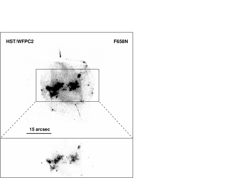
Figure 2: Grey-scale representation of the F685N HST/WFPC2 image of NGC 7354. The same features described from ground-based images can be identified here. The lower frame shows a lower contrast view of the equatorial region of NGC 7354.

Table 1: Dereddened emission-line fluxes (normalized to H$\beta\,=\,100$).

Ion	$\lambda$	fλ	A1	A2	A3	A4	A5	B1	B2	B3	B4	B5	B6
H$\gamma$	4340	0.157	$\cdots$	38.1	34.6	35.7	37.3	59.6	61.7	63.2	59.6	56.4	61.6
[O III]	4363	0.149	$\cdots$	13.5	14.1	18.3	15.4	18.7	25.1	27.3	18.8	17.3	18.2
He I	4471	0.115	$\cdots$	6.3	6.6	$\cdots$	$\cdots$	$\cdots$	$\cdots$	$\cdots$	6.9	$\cdots$	9.3
He II	4686	0.050	3.8	56.3	51.6	76.9	24.8	8.4	46.9	56.9	68.1	74.9	55.5
[Ar IV]	4711	0.042	$\cdots$	8.7	7.5	11.5	7.7	$\cdots$	8.3	9.4	9.4	10.3	7.6
[Ar IV]	4740	0.034	$\cdots$	9.3	7.1	10.9	6.6	$\cdots$	6.3	5.9	7.3	7.2	6.8
H$\beta$	4861	0.000	100.0	100.0	100.0	100.0	100.0	100.0	100.0	100.0	100.0	100.0	100.0
[O III]	4959	$-$0.026	476.1	411.5	408.1	404.8	457.8	454.3	493.0	450.3	395.1	381.2	452.4
[O III]	5007	$-$0.038	1394.9	1216.2	1202.8	1198.9	1358.4	1353.1	1452.8	1323.4	1169.0	1125.3	1333.3
[N II]	5755	$-$0.185	$\cdots$	0.5	0.9	0.3	0.8	$\cdots$	$\cdots$	0.6	$\cdots$	$\cdots$	1.1
He I	5876	$-$0.203	15.4	9.8	10.9	8.2	13.7	16.3	11.4	9.7	9.0	8.5	10.7
[O I]	6300	$-$0.263	5.2	$\cdots$	0.6	0.2	1.0	$\cdots$	0.4	0.4	0.2	$\cdots$	0.9
[S III]	6312	$-$0.264	$\cdots$	1.8	2.3	1.6	1.5	2.8	2.3	2.2	1.7	2.1	2.1
[O I]	6364	$-$0.271	$\cdots$	$\cdots$	0.2	$\cdots$	$\cdots$	$\cdots$	$\cdots$	$\cdots$	$\cdots$	$\cdots$	0.4
[N II]	6548	$-$0.296	27.2	5.0	14.7	5.7	8.5	6.9	4.5	4.5	4.4	3.9	13.3
H$\alpha$	6563	$-$0.298	285.0	278.4	283.4	281.8	279.3	281.5	280.2	276.5	280.7	280.9	281.8
[N II]	6584	$-$0.300	65.7	13.9	41.4	11.7	23.8	21.8	13.2	13.0	12.2	11.3	42.3
He I	6678	$-$0.313	5.3	2.9	3.0	2.6	4.4	4.0	3.3	3.0	2.8	2.6	3.2
[S II]	6717	$-$0.318	4.6	1.3	2.7	1.0	1.8	2.7	1.2	1.2	1.1	1.1	2.3
[S II]	6731	$-$0.320	5.5	1.7	3.9	1.4	2.1	2.8	1.6	1.6	1.6	1.5	3.4
He I	7065	$-$0.364	4.0	2.7	3.2	2.3	3.5	4.1	3.2	2.7	2.6	2.2	2.6
[Ar III]	7135	$-$0.374	14.1	15.1	17.0	15.3	16.4	17.2	16.7	15.5	15.0	14.0	15.6
[Ar IV]	7236	$-$0.387	$\cdots$	1.2	1.2	1.0	1.0	$\cdots$	0.9	1.2	1.5	1.2	1.1
He I	7281	$-$0.393	$\cdots$	0.4	0.5	0.4	0.8	$\cdots$	0.6	0.6	0.6	0.4	0.6
[O II]	7320	$-$0.398	1.6	1.0	1.5	1.0	1.4	1.6	0.9	1.2	1.2	1.0	1.4
[O II]	7330	$-$0.400	0.6	0.8	1.2	0.9	0.8	$\cdots$	$\cdots$	$\cdots$	$\cdots$	$\cdots$	$\cdots$
$c$(H$\beta$)			2.44	2.04	1.96	1.86	1.73	2.05	2.12	2.12	1.98	1.99	2.03
log $I$(H$\beta$)			-16.873	-14.998	-14.898	-15.040	-15.016	-15.901	-15.891	-15.461	-15.235	-15.311	-15.417

Table 2: —Continued

Ion	$\lambda$	fλ	B7	C1	C2	C3	C4	C5	C6	D1	D2	D3
H$\gamma$	4340	0.127	60.3	$\cdots$	58.4	69.6	48.9	49.2	55.8	77.9	57.7	60.9
[O III]	4363	0.121	23.7	$\cdots$	9.7	$\cdots$	14.5	23.1	13.0	15.4	$\cdots$	15.0
He I	4471	0.095	$\cdots$	$\cdots$	7.6	$\cdots$	$\cdots$	$\cdots$	$\cdots$	$\cdots$	$\cdots$	$\cdots$
He II	4686	0.043	8.6	1.4	34.8	39.9	58.0	63.1	22.7	6.7	7.3	9.0
[Ar IV]	4711	0.037	6.2	$\cdots$	11.1	13.7	8.3	8.6	$\cdots$	$\cdots$	$\cdots$	$\cdots$
[Ar IV]	4740	0.030	$\cdots$	$\cdots$	2.7	$\cdots$	6.5	8.3	7.4	$\cdots$	$\cdots$	$\cdots$
H$\beta$	4861	$-$0.000	100.0	100.0	100.0	100.0	100.0	100.0	100.0	100.0	100.0	100.0
[O III]	4959	$-$0.024	461.4	402.9	464.1	457.7	403.1	381.6	475.1	465.4	449.5	478.3
[O III]	5007	$-$0.036	1380.8	1193.7	1364.1	1352.5	1181.0	1127.9	1416.6	1384.9	1334.6	1403.1
[N II]	5755	$-$0.195	$\cdots$	1.2	1.6	1.3	1.5	0.8	$\cdots$	$\cdots$	$\cdots$	$\cdots$
He I	5876	$-$0.215	16.2	16.7	12.2	10.5	10.3	8.8	14.1	16.2	16.0	15.8
[O I]	6300	$-$0.282	0.4	1.6	2.6	1.8	2.4	0.8	0.3	0.4	$\cdots$	1.0
[S III]	6312	$-$0.283	2.1	1.8	2.2	2.3	2.3	2.0	1.9	1.5	2.2	1.5
[O I]	6364	$-$0.291	$\cdots$	$\cdots$	0.9	1.0	0.7	0.2	$\cdots$	$\cdots$	$\cdots$	$\cdots$
[N II]	6548	$-$0.318	8.0	20.8	28.2	22.1	26.8	10.5	7.0	18.4	5.8	8.8
H$\alpha$	6563	$-$0.320	280.2	284.2	283.5	283.5	283.9	282.0	283.5	282.7	285.0	283.0
[N II]	6584	$-$0.323	24.5	65.2	82.8	66.6	82.8	31.8	21.0	58.4	19.5	28.2
He I	6678	$-$0.336	4.1	4.4	3.5	3.5	3.2	2.7	4.2	4.6	4.5	5.1
[S II]	6717	$-$0.342	1.9	3.5	3.6	2.8	3.4	1.8	2.2	4.2	1.9	2.1
[S II]	6731	$-$0.344	2.5	5.6	5.0	4.1	5.1	2.7	2.2	5.3	2.5	3.4
He I	7065	$-$0.387	3.6	4.2	3.5	3.3	3.3	2.6	3.3	4.2	4.5	3.7
[Ar III]	7135	$-$0.396	16.0	19.6	18.0	17.3	17.2	15.2	14.5	18.7	15.9	15.8
[Ar IV]	7236	$-$0.409	0.5	$\cdots$	0.9	1.1	1.0	1.3	$\cdots$	$\cdots$	$\cdots$	$\cdots$
He I	7281	$-$0.414	0.7	$\cdots$	0.6	0.5	0.4	0.6	$\cdots$	$\cdots$	1.4	0.4
[O II]	7320	$-$0.419	1.0	1.6	2.3	2.0	1.9	1.2	0.5	2.9	1.1	0.6
[O II]	7330	$-$0.420	$\cdots$	1.4	2.1	2.1	2.3	1.3	1.4	$\cdots$	$\cdots$	$\cdots$
$c$(H$\beta$)			2.01	2.20	2.41	2.24	1.95	2.02	1.71	1.78	1.83	1.83
log $I$(H$\beta$)			-15.801	-16.357	-16.056	-16.224	-15.203	-15.313	-15.399	-15.967	-15.874	-15.913

Table 3: Derived physical parameters.

Region		$T_{\rm{}_{e}}$ [K]			$N_{\rm{}_{e}}$ [cm-3]
		[N II]	[O III]		[S II]	[Cl III]	[Ar IV]
A1		$\cdots$	$\cdots$		1141$\pm$1080	$\cdots$	$\cdots$
A2		15909$\pm$1149	12040$\pm$243		2048$\pm$350	5545$\pm$ 2660	5658$\pm$1319
A3		11459$\pm$386	12281$\pm$262		2623$\pm$281	4023$\pm$ 1888	3754$\pm$1436
A4		12870$\pm$1404	13618$\pm$322		1982$\pm$557	1033$\pm$952	3812$\pm$1201
A5		15125$\pm$1920	12135$\pm$447		1404$\pm$458	$\cdots$	2341$\pm$1587
B1		$\cdots$	13130$\pm$700		751$\pm$267	$\cdots$	$\cdots$
B2		$\cdots$	14346$\pm$519		1799$\pm$610	$\cdots$	$\cdots$
B3		17690$\pm$1468	15523$\pm$356		2402$\pm$515	$\cdots$	$\cdots$
B4		$\cdots$	13885$\pm$263		3106$\pm$555	7708$\pm$4389	1062$\pm$767
B5		$\cdots$	13646$\pm$286		2216$\pm$415	15086$\pm$9695	$\cdots$
B6		12833$\pm$567	13005$\pm$298		2700$\pm$356	$\cdots$	2986$\pm$1423
B7		$\cdots$	14334$\pm$956		1910$\pm$636	$\cdots$	$\cdots$
C1		10724$\pm$2902	$\cdots$		3451$\pm$4044	$\cdots$	$\cdots$
C2		11312$\pm$785	10363$\pm$1162		2130$\pm$629	$\cdots$	$\cdots$
C3		11329$\pm$1438	$\cdots$		2354$\pm$1194	$\cdots$	$\cdots$
C4		11006$\pm$481	12478$\pm$755		2715$\pm$551	$\cdots$	$\cdots$
C5		12662$\pm$1271	15454$\pm$1039		3311$\pm$1290	$\cdots$	$\cdots$
C6		$\cdots$	11298$\pm$1564		664$\pm$910	$\cdots$	$\cdots$
D1		$\cdots$	12066$\pm$984		1603$\pm$575	$\cdots$	$\cdots$
D2		$\cdots$	$\cdots$		1574$\pm$725	$\cdots$	$\cdots$
D3		$\cdots$	11825$\pm$835		4102$\pm$2481	$\cdots$	$\cdots$

Table 4: Derived ionic abundances.

Region	Ion
	He+	He++	N+	O0	O+1	O+2	S+	S+2	Ar+2	Ar+3	Ar+4
			[1$\times 10^{-5}$]	[1$\times 10^{-6}$]	[1$\times 10^{-5}$]	[1$\times 10^{-4}$]	[1$\times 10^{-7}$]	[1$\times 10^{-6}$]	[1$\times 10^{-6}$]	[1$\times 10^{-6}$]	[1$\times 10^{-7}$]
A1	0.117	0.003	1.38	10.12	2.98	4.89	2.83	$\cdots$	1.30	$\cdots$	$\cdots$
A2	0.073	0.046	0.10	$\cdots$	0.18	1.10	0.37	0.80	0.55	0.49	0.69
A3	0.074	0.042	0.60	0.74	1.11	2.69	1.63	3.17	1.15	0.91	1.00
A4	0.058	0.062	0.13	0.15	0.49	1.90	0.42	1.47	0.82	1.04	1.06
A5	0.099	0.020	0.19	0.50	0.28	1.40	0.47	0.81	0.65	0.46	$\cdots$
B1	0.112	0.007	0.42	$\cdots$	3.98	4.76	1.45	6.68	1.59	$\cdots$	$\cdots$
B2	0.082	0.038	0.26	0.72	1.60	5.15	0.87	5.54	1.54	1.32	$\cdots$
B3	0.062	0.048	0.08	0.11	0.13	0.94	0.30	0.74	0.48	0.37	0.39
B4	0.069	0.055	0.25	0.35	1.86	4.14	0.99	3.99	1.39	1.54	2.50
B5	0.061	0.061	0.23	$\cdots$	1.71	3.98	0.82	4.88	1.29	1.60	2.90
B6	0.074	0.045	0.46	0.86	0.57	2.13	1.12	1.89	0.84	0.67	0.85
B7	0.110	0.007	0.48	0.74	1.88	4.84	1.39	4.89	1.48	1.03	$\cdots$
C1	0.110	0.001	1.11	2.46	1.56	3.29	2.87	3.08	1.53	$\cdots$	$\cdots$
C2	0.083	0.028	1.21	3.22	2.13	3.08	2.06	3.22	1.26	1.32	0.88
C3	0.088	0.032	0.98	3.41	1.96	3.14	1.69	3.27	1.20	1.64	1.11
C4	0.080	0.047	1.31	3.18	2.46	3.01	2.35	3.69	1.27	1.02	1.07
C5	0.068	0.051	0.36	0.63	0.60	1.89	0.98	1.92	0.84	0.81	1.64
C6	0.101	0.018	0.41	0.67	1.34	4.98	1.15	4.69	1.33	1.56	$\cdots$
D1	0.116	0.005	1.13	0.69	5.51	4.88	2.85	3.51	1.73	$\cdots$	$\cdots$
D2	0.113	0.006	0.38	$\cdots$	2.18	4.65	1.31	5.21	1.46	$\cdots$	$\cdots$
D3	0.113	0.007	0.57	1.88	0.87	4.92	2.16	3.51	1.45	$\cdots$	$\cdots$

Note. — In regions A5, B1 and D3, He⁺⁺ abundances shown are an upper limit.

Table 5: Derived total abundances.

Region	He/H	O/H	N/H	S/H	Ar/H
A1	0.120$\pm$0.010	8.72$\pm$0.05	8.39$\pm$0.35	6.67$\pm$1.54	6.38$\pm$0.10
A2	0.118$\pm$0.001	8.19$\pm$0.14	7.94$\pm$0.28	6.41$\pm$0.14	6.05$\pm$0.01
A3	0.116$\pm$0.001	8.58$\pm$0.15	8.31$\pm$0.21	6.88$\pm$0.09	6.35$\pm$0.01
A4	0.121$\pm$0.001	8.50$\pm$0.40	7.94$\pm$0.60	6.63$\pm$0.27	6.30$\pm$0.01
A5	0.119$\pm$0.001	8.21$\pm$0.28	8.02$\pm$0.59	6.36$\pm$0.28	6.09$\pm$0.14
B1	0.118$\pm$0.002	8.73$\pm$0.11	7.76$\pm$0.13	7.06$\pm$0.05	6.47$\pm$0.10
B2	0.120$\pm$0.002	8.84$\pm$0.08	8.05$\pm$0.12	7.14$\pm$0.04	6.46$\pm$0.10
B3	0.110$\pm$0.001	8.15$\pm$0.18	7.90$\pm$0.26	6.40$\pm$0.14	5.95$\pm$0.01
B4	0.124$\pm$0.001	8.81$\pm$0.04	7.94$\pm$0.07	6.97$\pm$0.03	6.51$\pm$0.01
B5	0.122$\pm$0.001	8.82$\pm$0.05	7.94$\pm$0.07	7.07$\pm$0.03	6.51$\pm$0.01
B6	0.119$\pm$0.001	8.48$\pm$0.15	8.38$\pm$0.21	6.72$\pm$0.10	6.21$\pm$0.01
B7	0.117$\pm$0.002	8.72$\pm$0.16	8.13$\pm$0.18	7.03$\pm$0.07	6.44$\pm$0.10
C1	0.111$\pm$0.006	8.54$\pm$0.89	8.39$\pm$4.87	6.82$\pm$1.90	6.46$\pm$0.40
C2	0.111$\pm$0.003	8.60$\pm$0.30	8.36$\pm$0.45	6.81$\pm$0.20	6.45$\pm$0.03
C3	0.120$\pm$0.006	8.61$\pm$0.27	8.31$\pm$0.74	6.83$\pm$0.36	6.49$\pm$0.04
C4	0.127$\pm$0.002	8.65$\pm$0.26	8.37$\pm$0.33	6.86$\pm$0.14	6.41$\pm$0.02
C5	0.120$\pm$0.003	8.45$\pm$0.55	8.23$\pm$0.72	6.71$\pm$0.29	6.27$\pm$0.02
C6	0.120$\pm$0.005	8.76$\pm$0.23	8.25$\pm$0.97	7.07$\pm$0.33	6.40$\pm$0.10
D1	0.122$\pm$0.007	8.75$\pm$0.14	8.06$\pm$0.16	6.77$\pm$0.08	6.51$\pm$0.10
D2	0.118$\pm$0.002	8.70$\pm$0.01	7.94$\pm$0.13	7.03$\pm$0.06	6.44$\pm$0.10
D3	0.120$\pm$0.002	8.72$\pm$0.13	8.53$\pm$0.17	7.01$\pm$0.09	6.43$\pm$0.10
PNea	0.12$\pm$0.02	8.68$\pm$0.15	8.35$\pm$0.25	6.92$\pm$0.30	6.39$\pm$0.30
TI PNeb	0.13$\pm$0.04	8.65$\pm$0.15	8.72$\pm$0.15	6.91$\pm$0.30	6.42$\pm$0.30
H IIc	0.10$\pm$0.01	8.70$\pm$0.04	7.57$\pm$0.04	7.06$\pm$0.06	6.42$\pm$0.04
Sund	0.09$\pm$0.01	8.66$\pm$0.05	7.78$\pm$0.06	7.14$\pm$0.05	6.18$\pm$0.08

Note. — Except for He, all abundances relative to H are logarithmic values with logH = +12. Final rows are for comparison: (a) Average for PNe (Kingsburgh & Barlow, 1994); (b) Average for Type I PNe (Kingsburgh & Barlow, 1994); (c) Average for H II regions (Shaver et al., 1983); the Sun (Grevesse, Asplund & Sauval, 2007). In regions A5, B1, and D3, He abundances shown are an upper limit.

Table 6: Geometrical and Kinematic Parameters from our SHAPE model.

Geometrical Structure	Size	Expansion Velocity	Inclination Angle $i$	Position Angle $\phi$	Kinematical Age
	[′′]	[km s-1]	[deg]	[deg]	[yr]
Outer Elliptical Shell	16 $\times$ 15	45	94	18	2 500
Inner Elliptical Shell	10 $\times$ 8	35	94	28	1 600
Semispherical cap N	14	47	94	28	1 000
Semispherical cap S	14	47	85	203	1 000
Spherical Knots	1 to 2	25 to 44	$\cdots$	$\cdots$
Thin Cylinder N	7	60	95	3	1 900
Thin Cylinder S	13	60	85	205	1 900

Note. — Size refers to major and minor axis in the case of elliptical structures, length for thin cylinders, and diameter in the case of the spherical knots and polar caps. All kinematical ages were determined assuming a distance to the nebula of 1.5 kpc (Sabbadin, 1986).

References

- Akashi & Soker (2008) Akashi, M. & Soker, N. 2008, MNRAS, 391, 1063
- Balick (1987) Balick, B. 1987, AJ, 94, 671
- Balick et al. (1987) Balick, B., Preston, H.L. & Icke, V. 1987, AJ, 94, 1641
- Balick & Frank (2002) Balick, B. & Frank, A. 2002, ARA&A, 40, 439
- Cahn et al. (1992) Cahn, J.H., Kaler, J.B. & Stanghellini, L. 1992, A&AS, 94, 399
- Cardelli, Clayton & Mathis (1989) Cardelli, J.A., Clayton, G.C. & Mathis, J.S. 1989, ApJ, 345, 245
- Daub (1982) Daub, C.T. 1982, ApJ, 260, 612
- Dennis et al. (2008) Dennis, T.J., Cunningham, A.J., Frank, A., Balick, B., Blackman, E.G. & Mitran, S. 2008, ApJ, 679, 1327
- DeRobertis, Dufour & Hunt (1987) DeRobertis, M.M., Dufour, R. & Hunt, R. 1987, JRASC, 81, 195
- Frank et al. (1996) Frank, A., Balick, B. & Livio, M. 1996, ApJ, 471, L53
- García-Arredondo & Frank (2004) García-Arredondo, F. & Frank, A. 2004, ApJ, 600, 992
- Grevesse, Asplund & Sauval (2007) Grevesse, N., Asplund, M. & Sauval, A.J. 2007, Space Sci. Rev., 130, 105
- Guerrero et al. (2008) Guerrero, M.A., Miranda, L.F., Riera, A., Velázquez, P.F., Olguín, L., Vázquez, R., Chu, Y.-H., Raga, A., Benítez, G. 2008, ApJ, 683, 272
- Hajian et al. (1997) Hajian, A.R., Balick, B., Terzian, Y. & Perinotto, M. 1997 ApJ, 487, 304
- Hajian et al. (2007) Hajian, A.R., Movit, S.M., Trofimov, D., Balick, B., Terzian, Y., Knuth, K.H., Granquist-Fraser, D., Huyser, K.A., Jalobeanu, A., McIntosh, D., Jaskot, A.E., Palen, S. & Panagia, N. 2007, ApJS, 169, 289
- Kingsburgh & Barlow (1994) Kingsburgh, R.L. & Barlow, M.J. 1994,MNRAS, 271,257
- Kwok et al. (1978) Kwok, S., Purton, C.R. & Fitzgerald, P.M. 1978, ApJ, 219, L125
- Lee & Sahai (2003) Lee, C.-F. & Sahai, R. 2003, ApJ, 586, 319
- López et al. (2000) López, J. A., Meaburn, J., Rodríguez, L. F., Vázquez, R., Steffen, W., Bryce M. 2000, ApJ, 538, 233
- Manchado et al. (1996) Manchado, A., Guerrero, M.A., Stanghellini, L. & Serra- Ricart, M. 1996, The IAC morpholigical catalog of northern Galactic planetary nebulae, Pub. La Laguna, Spain:Instituto Astrofísico de Canarias
- Martins & Viegas (2002) Martins, L.P. & Viegas, S.M. 2002, A&A, 387, 1074
- Meaburn et al. (2003) Meaburn, J., López, J.A., Gutiérrez, L. et al. 2003, Rev. Mexicana Astron. Astrofis., 39, 185
- Mellema (1995) Mellema, G. 1995, MNRAS, 277, 173
- Mellema & Frank (1995) Mellema, G. & Frank, A. 1995, MNRAS, 273, 401
- Mezger & Henderson (1967) Mezger, P.G. & Henderson, A.P. 1967, ApJ, 147, 471
- Miranda & Solf (1992) Miranda, L.F. & Solf, J. 1992, A&A, 260, 397
- Miranda et al. (2006) Miranda, L.F., Ayala, S., Vázquez, R. & Guillén, P.F. 2006, A&A, 456, 591
- Miranda, Pereira & Guerrero (2009) Miranda, L.F., Pereira, C.B. & Guerrero, M.A. 2009, AJ, 137, 414
- O’Dell et al. (2002) O’Dell, C.R., Balick, B., Hajian, A.R., Henney, W.J. & Burkert, A. 2002, AJ, 123, 3329
- Perinotto et al. (2004a) Perinotto, M., Morbidelli, L. & Scatarzi, A. 2004a, MNRAS, 349, 793
- Perinotto et al. (2004b) Perinotto, M., Patriarchi, P., Balick, B. & Corradi, R.L.M. 2004b, A&A, 422, 963
- Phillips (2004) Phillips, J.P. 2004, MNRAS, 353, 589
- Phillips et al. (2009) Phillips, J.P., Ramos-Larios, G., Schröeder, K.-P. & Contreras, J.L. Verbena 2009, MNRAS, 399, 1126
- Rasio & Livio (1996) Rasio, F.A. & Livio, M. 1996, ApJ, 4 71, 366
- Sabbadin (1986) Sabbadin, F. 1986, A&AS, 64, 579
- Sabbadin et al. (1983) Sabbadin, F., Bianchini, A. & Hamzaoglu, E. 1983, A&A, 51, 119
- Sahai & Trauger (1998) Sahai, R. & Trauger, John T. 1998, AJ, 116, 1357
- Sahai et al. (2007) Sahai, R., Morris, M., Sánchez Contreras, C. & Claussen, M. 2007, AJ, 134, 2200
- Sandquist et al. (1998) Sandquist, E.L., Taam, R.E., Chen, X., Bodenheimer, P. & Burkert, A. 1998, ApJ, 500, 909
- Schwarz et al. (1992) Schwarz, H.E., Corradi, R. & Melnick, J. 1992, A&AS, 96, 23
- Shaver et al. (1983) Shaver, P.A., McGee, R.X., Newton, L.M., Danks, A.C. & Pottasch, S.R. 1983, MNRAS, 204,53
- Shaw & Dufour (1994) Shaw, R.A. & Dufour, R.J. 1994, in D.R. Crabtree, Hanisch, R.J., Barnes, J., eds., ASP Conf. Ser. Vol. 61, Astronomical Data Analysis Software and Systems III. Astron. Soc. Pac., San Francisco, p.327
- Soker & Livio (1994) Soker, N. & Livio, M. 1994, ApJ, 421, 219
- Soker & Rappaport (2000) Soker, N. & Rappaport, S. 2000, ApJ, 538, 241
- Stanghellini et al. (2006) Stanghellini, L., Guerrero, M.A., Cunha, K., Manchado, A. & Villaver, E. 2006, ApJ, 651, 898
- Steffen & López (2006) Steffen, W. & López, J.A. 2006, Rev. Mexicana Astron. Astrofis., 42, 99
- Terman & Taam (1996) Terman, J.L. & Taam, R.E. 1996, ApJ, 458, 692
- Terzian et al. (1974) Terzian, Y., Balick, B., & Bignell, C. 1974, ApJ, 188, 257
- Vázquez et al. (1998) Vázquez R., Kingsburgh R.L., López J.A. 1998, MNRAS, 296, 564
- Vázquez et al. (1999) Vázquez R., López J.A., Miranda, L.F., Torrelles, J.M., Meaburn, J. 1999, MNRAS, 308, 939
- Vázquez et al. (2008) Vázquez R., Miranda, L.F., Olguín, L., Ayala, S., Torrelles, J.M., Contreras, M.E. and Guillén, P.F. 2008, A&A, 481, 107
- Zhang (1995) Zhang, C.Y. 1995, ApJS, 98, 659