Diffraction of light by a planar aperture in a metallic screen

Abstract

We present a complete derivation of the formula of Smythe [Phys. Rev. 72, 1066 (1947)] giving the electromagnetic field diffracted by an aperture created in a perfectly conducting plane surface. The reasoning, valid for any excitating field and any hole shape, makes use only of the free scalar Green function for the Helmoltz equation without any reference to a Green dyadic formalism. We compare our proof with the one previously given by Jackson and connect our reasoning to the general Huygens Fresnel theorem.

I Introduction

Diffraction of electromagnetic waves by an aperture in a perfect metallic plane is not only a mathematical problem of fundamental interest but is connected to many applications in the microwave domain (for example, in waveguides and in cavity resonators Collin ) as well as in the optical regime where it is involved in many optical arrangements Born . The fundamental importance of this phenomenon in near-field optics has been pointed out as early as in 1928 by Synge Synge in his prophetic paper and is currently involved in modern near-field scanning optical microscopy (NSOM) Pohl .
In the domain of applicability of NSOM where distances and dimensions are smaller than or close to the wavelength of light, we need to know the exact structure of the electromagnetic field, and we cannot in general consider the usual approximations involved in Kirchhoff’s theory for a scalar wave Drezet1 ; Drezet2 ; Drezet3 . In this context, one of the most cited approaches is the one given by Bethe Bethe in 1944 and corrected by Bouwkamp Bouwkamp1 ; Bouwkamp2 . It gives the electromagnetic field diffracted by a small circular aperture in a perfect metallic plane in the limit where the optical wavelength is much larger than the aperture. Less known is the more general formula of Smythe Smythe ; Smythe2 which expresses in a formal way the Huygens Fresnel principle for any kind of aperture in a metallic screen. Even if this formula is not an explicit solution for the general diffraction problem, it constitutes an integral equation which can be used in a self consistent way in perturbative or numerical calculations of the diffracted field Butler ; Eggimann . Further efforts have been made by Smythe Smythe ; Smythe2 himself in order to justify his formula by means of some arrangements of current sheets fitting the aperture. This method essentially consists of transforming the problem of diffraction by a hole into a physically different one in order to guess the correct integral equation for the original problem. However, if this physical reasoning proves the consistency of the proposed solution with Maxwell equations and boundary conditions for the field, it is not directly connected to the rigorous electromagnetic formulation of the Huygens Fresnel principle obtained by Stratton and Chu  Stratton . Such a connection is expected naturally because these two formulations of diffraction must be equivalent here.
Jackson  Jackson , in the first edition of his textbook on electrodynamics, developed a complete proof of the Smythe formula starting from the Stratton and Chu formula [Eq. (3) of the present paper]. Nevertheless, like in the original paper of Smythe, Jackson transforms the problem into a physically different one in order to guess the correct result. The result is then subjected to the same remarks as above for Smythe’s approach. Other justifications of Smythe results are based on the use of the Babinet theorem or of the Green dyadic method. The latter, which uses a tensorial Green function instead of a scalar one like in Kirchhoff’s or Stratton and Chu’s theories, gives us the most direct justification for Smythe approach in terms of the Huygens Fresnel principle. However, this proof is for the moment not directly connected to the Stratton and Chu approach. It is the aim of this paper to establish such a link.
The paper is organized as follows. We give in Sec. II a description of the general theory of diffraction of electromagnetic waves by an aperture in a screen. In Sec. III, we exploit precedent works by Jackson  Jackson ; Jackson2 and Levine and Schwinger  Levine to justify directly and rigorously the Smythe formula using the Stratton Chu theorem without relying on any ingenious physical “trick”. Sec. IV deals with a vectorial justification of Smythe’s approach. The consistency between the various theoretical treatments of diffraction by an aperture in a metallic screen is stressed in Sec. V which also compares our treatment with that obtained within the Green dyadic formalism  Schwinger1 ; Schwinger2 . Our conclusions appear in Section VI.

II The diffraction problem in electromagnetism

The first coherent theory of diffraction was elaborated by Kirchhoff (1882) on the basis of the Huygens Fresnel principle  Born ; Poincare . The method of integral equations allows one to write a solution $\psi\left(\vec{r}\right)e^{-i\omega t}$ of the Helmholtz propagation equation $[\nabla^{2}+k^{2}]\psi\left(\vec{r}\right)=0$ ($k=\omega/c$) using the “free” scalar Green function $G\left(\vec{r},\vec{r^{\prime}}\right)=e^{ikR}/4\pi R$ which is a solution of the equation $[\nabla^{2}+k^{2}]G\left(\vec{r},\vec{r^{\prime}}\right)=-\delta^{3}\left(\vec{r}-\vec{r^{\prime}}\right)$.
If, as schematized in Fig. 1, we consider now an aperture $\delta S$ made in a two-dimensional infinite screen $S$ and illuminated by incident radiation, we can express the field $\psi$ existing at each observation point located behind the screen (i. e. , for $z>0$) by the Kirchhoff formula

$$\psi\left(\vec{r}\right)=\int_{S}[\psi\left(\vec{r^{\prime}}\right)\vec{n^{\prime}}\cdot\overrightarrow{\nabla^{\prime}}G\left(\vec{r},\vec{r^{\prime}}\right)-G\left(\vec{r},\vec{r^{\prime}}\right)\vec{n^{\prime}}\cdot\overrightarrow{\nabla^{\prime}}\psi\left(\vec{r^{\prime}}\right)]\textrm{d}S^{\prime},$$ (1)

where the normal unit vector ${n^{\prime}}$ is oriented into the diffraction half-space.
In a problem of diffraction, we usually impose the additional first Kirchhoff “shadow” approximation $\psi\left(\vec{r^{\prime}}\right)=\partial_{n^{\prime}}\psi\left(\vec{r^{\prime}}\right)=0$ which is valid on the unilluminated side of the screen. This permits one to restrict the integral in (1) to the region of the aperture only, which is very useful in some approximations or iterative resolutions. Nevertheless, this intuitive hypothesis has some fundamental inconsistencies because, following a theorem due to Poincaré Poincare , a field satisfying the shadow approximation on a finite domain must vanish everywhere.
A classic solution proposed by Rayleigh Rayleigh and Sommerfeld Sommerfeld to circumvent this difficulty consists in replacing the free Green function by the Dirichlet $G_{D}$ or the Neumann $G_{N}$ Green functions Jackson satisfying $\partial_{n^{\prime}}G_{N}\left(\vec{r},\vec{r^{\prime}}\right)=0$ and $G_{D}\left(\vec{r},\vec{r^{\prime}}\right)=0$ for all points $\vec{r^{\prime}}$ on $S$. We can then rigourously reduce the integral to the region of the aperture depending on the nature of the boundary problem. For example, if we impose $\psi=0$ on the screen, we can then write

$$\psi\left(\vec{r}\right)=\int_{\textrm{Aperture}}\psi\left(\vec{r^{\prime}}\right)\partial_{n^{\prime}}G_{D}\left(\vec{r},\vec{r^{\prime}}\right)\textrm{d}S^{\prime}.$$ (2)

In principle, it could be possible to generalize the preceding methods to the different Cartesian components $\psi_{\alpha}$ of the electromagnetic field using equations of the form $\psi_{\alpha}=\int_{S}[\psi_{\alpha}\partial_{n^{\prime}}G-G\partial_{n^{\prime}}\psi_{\alpha}]\textrm{d}S^{\prime}$. Nevertheless, as pointed out by Stratton, Chu  Stratton and others  Love ; Larmor ; Kottler , the Maxwell equations couple the field components between them and the consistency of these relations must be controlled if we use an integral equation like Eq. (1) either in an exact or approximative treatment of diffraction. In addition, because the boundary conditions imposed by Maxwell’s equations connect the tangential and the normal components of the field on the screen surface, it is not at all trivial to reduce the integral to the region of the aperture directly using Eq. (1).
Due to the uniqueness theorem, such possible reduction of the integral appearing in the Huygens Fresnel principle is expected in the case of a perfectly conducting metallic screen. Indeed, following this uniqueness theorem, the field in the diffracted space must depend only on the tangential electric field on the screen and aperture surface. Because the tangential electric field vanishes on the screen, the integral must depend only on the tangential field at the opening.
Numerous authors, especially Stratton and Chu  Stratton as well as Schelkunoff  Schelkunoff ; Schelkunoff2 , have discussed a vectorial integral equation satisfying Maxwell’s equations automatically. We can effectively write

$$\overrightarrow{E}\left(\vec{x}\right)=\int_{S}[ik\left(\vec{n^{\prime}}\times\overrightarrow{B}\right)G+\left(\vec{n^{\prime}}\times\overrightarrow{E}\right)\times\overrightarrow{\nabla^{\prime}}G+$$

$$\left(\vec{n^{\prime}}\cdot\overrightarrow{E}\right)\overrightarrow{\nabla^{\prime}}G]\textrm{d}S^{\prime},$$ (3)

hereafter referred to as the Stratton Chu equation. A similar expression holds for the magnetic field by means of the substitution $\overrightarrow{E}\rightarrow\overrightarrow{B}$ and $\overrightarrow{B}\rightarrow-\overrightarrow{E}$.
It is important to note that Eq. (3) is over-determined although it depends explicitly on the tangential and normal components of the electromagnetic field defined on $S$. Indeed, due to the equivalence principle of Love and Schelkunoff  Love ; Schelkunoff ; Stratton2 and to the uniqueness theorem, we expect that the “most adapted” integral equations depend only on $\vec{n^{\prime}}\times\overrightarrow{E}$ or $\vec{n^{\prime}}\times\overrightarrow{B}$ on $S$. In addition, unlike in the scalar case, we cannot directly reduce the surface integral to the region of the aperture just by choosing an adapted Dirichlet or Neumann Green function. It seems then necessary to apply once again the shadow approximation of Kirchhoff in order to simplify the integration despite the inconsistency of the method. As in the Poincaré theorem, some problems appear here because we need to add a nonphysical contour integral associated with a magnetic line charge in Eq. (3) (or to an electric line charge in the equivalent formula for ${B}$) in order to satisfy Maxwell’s equations and to compensate for the arbitrary change imposed to the integration domain Meixner . Furthermore, in this Kirchhoff Kottler Kottler theory, the introduction of contour integrals induces a logarithmic divergence of the energy at the rim of the aperture, a fact which is forbidden in a diffraction problem.
The particular case of the diffraction by an aperture in a planar screen constitutes an exception in the sense that a rigorous integral equation had been anticipated by Schelkunoff  Schelkunoff and Bethe  Bethe for a subwavelength circular aperture and generalized by Smythe  Smythe ; Smythe2 for any kind of aperture. The integral equation is

$$\overrightarrow{E}\left(\vec{x}\right)=\frac{1}{2\pi}\overrightarrow{\nabla}\times\Big{(}\int_{\texttt{Aperture}}\left({\hat{z}}\times\overrightarrow{E}\right)\frac{e^{ikR}}{R}\textrm{d}S^{\prime}\Big{)}.$$ (4)

For some applications, it is important to note that in the short wavelength limit ($\lambda\ll\textrm{aperture typical radius}$) for which the electromagnetic field in the aperture can be identified with the incident plane wave $\overrightarrow{B}_{i}={\hat{z}}\times\overrightarrow{E}_{i}$ (first Kirchhoff approximation), the formula of Stratton Chu limited to the aperture domain and the exact solution of Smythe give approximately the same result. Indeed, within the Fraunhofer approximation, Eq. (4) reads

$$\overrightarrow{E}\simeq\frac{ike^{ikr}}{r}{\hat{r}}\times\int_{\texttt{Aperture}}\Big{(}\frac{{\hat{z}}\times\overrightarrow{E}_{i}}{2\pi}e^{-ik{\hat{r}}\cdot\overrightarrow{x^{\prime}}}\Big{)}\textrm{d}S^{\prime},$$ (5)

whereas Eq. (3) reduces to

$$\overrightarrow{E}\simeq\frac{ike^{ikr}}{r}\frac{{\hat{r}}+{\hat{z}}}{2}\times\int_{\texttt{Aperture}}\Big{(}\frac{{\hat{z}}\times\overrightarrow{E}_{i}}{2\pi}e^{-ik{\hat{r}}\cdot\vec{x^{\prime}}}\Big{)}\textrm{d}S^{\prime}.$$ (6)

Both equations are identical in the practical limit of small diffraction angles, i. e. , close to the normal axis $z$ going through the aperture. Equation (5) is correct for a subwalength aperture only because we cannot identify the field in the aperture with the incident one. We can see that the asymptotic diffracted field for $z>0$ is equivalent to the one produced by an effective magnetic dipole

$$\overrightarrow{M}_{\textrm{eff}}=\int_{\texttt{Aperture}}\Big{(}\frac{\vec{n^{\prime}}\times\overrightarrow{E}}{2\pi ik}\Big{)}\textrm{d}S^{\prime},$$ (7)

and by an effective electric dipole

$$\overrightarrow{P}_{\textrm{eff}}=\frac{{\hat{z}}}{4\pi}\int_{\texttt{Aperture}}\left(\vec{x^{\prime}}\cdot\overrightarrow{E}\right)\textrm{d}S^{\prime}.$$ (8)

These formula are fundamental in the context of NSOM because they give us the Bethe Bouwkamp Bethe ; Bouwkamp1 ; Bouwkamp2 ; Jackson dipoles which, in the particular case of a circular aperture of radius $a$, are

$$\overrightarrow{P}_{\textrm{eff}}=\frac{a^{3}}{3\pi}\overrightarrow{E}_{\bot}^{\left(0\right)}\quad,\overrightarrow{M}_{\textrm{eff}}=-\frac{2a^{3}}{3\pi}\overrightarrow{B}_{\|}^{\left(0\right)}.$$ (9)

$\overrightarrow{E}_{\bot}^{\left(0\right)}$ and $\overrightarrow{B}_{\|}^{\left(0\right)}$ are, respectively, the locally uniform normal electric field and tangential magnetic field existing in the aperture zone in the absence of the opening (in $z=0^{-}$).

III Green dyadic justification of the Smythe formula

The so-called Smythe formula Eq. (4) is generally obtained on the basis of different principles such as the Babinet principle or the equivalence theorem (see Schelkunoff  Schelkunoff , Bouwkamp  Bouwkamp3 , Jackson  Jackson2 ). In particular, the equivalence theorem shows that the solution of Smythe for $z>0$ is identical to the one obtained by considering a virtual surface magnetic-current density given by $\overrightarrow{J}_{s}^{m}=-c{\hat{z}}\times\overrightarrow{E}/\left(2\pi\right)$. All these derivations are self consistent if we consider the very fact that the guessed results fulfill Maxwell equations. Then, the uniqueness theorem ensures that the result is the only one possible. Nevertheless, as already noted, the calculation is not direct and not necessarily connected to the Stratton and Chu formalism. A classical calculation due to Schwinger and Levine  Schwinger1 ; Schwinger2 shows, however, that it is possible to rigourously and directly obtain this equation using the tensorial, or dyadic, Green function formalism.
Such an electric dyadic Green function  Chentotai $\stackrel{{\scriptstyle\leftrightarrow}}{{G}}_{e}$, which is solution of the equation

$$\overrightarrow{\nabla}\times\left(\overrightarrow{\nabla}\times\stackrel{{\scriptstyle\leftrightarrow}}{{G}}_{e}\left({r},{r^{\prime}}\right)\right)=k^{2}\stackrel{{\scriptstyle\leftrightarrow}}{{G}}_{e}\left(\vec{r},\vec{r^{\prime}}\right)+\stackrel{{\scriptstyle\leftrightarrow}}{{\delta}}\delta^{3}\left(\vec{r}-\vec{r^{\prime}}\right)$$ (10)

(with $\stackrel{{\scriptstyle\leftrightarrow}}{{\delta}}=\sum_{i}{\hat{x}}_{i}{\hat{x}}_{i}$) satisfying the condition $\overrightarrow{\nabla}\cdot\stackrel{{\scriptstyle\leftrightarrow}}{{{G}}}_{e}=-\left(1/k^{2}\right)\overrightarrow{\nabla}\delta^{3}\left(\vec{r}-\vec{r^{\prime}}\right)$, can be used to write the integral equation

$$\overrightarrow{E}\left(\vec{r}\right)=\int_{S}[\left(\vec{n^{\prime}}\times\overrightarrow{E}\right)\cdot\overrightarrow{\nabla^{\prime}}\times\stackrel{{\scriptstyle\leftrightarrow}}{{{G}}}_{e}-ik\overrightarrow{B}\cdot\left(\vec{n^{\prime}}\times\stackrel{{\scriptstyle\leftrightarrow}}{{{G}}}_{e}\right)]\textrm{d}S^{\prime}$$ (11)

which is defined on the same surface as previously. By imposing the dyadic Dirichlet condition $\vec{n^{\prime}}\times\stackrel{{\scriptstyle\leftrightarrow}}{{{G}}}_{e}=0$ on $S$, we can obtain the relation

$$\overrightarrow{E}\left(\vec{r}\right)=\int_{\texttt{Aperture}}[\left(\vec{n^{\prime}}\times\overrightarrow{E}\right)\cdot\overrightarrow{\nabla^{\prime}}\times\stackrel{{\scriptstyle\leftrightarrow}}{{{G}}}_{e}]\textrm{d}S^{\prime}$$ (12)

which depends only on the tangential electric field at the aperture. This is in perfect agreement with the equivalence principle and the uniqueness theorem.
Following Ref.  Chentotai , the total Green function $\stackrel{{\scriptstyle\leftrightarrow}}{{{G}}}_{e}$ for the plane can be deduced from the “free” dyadic

$$\stackrel{{\scriptstyle\leftrightarrow}}{{{G}}}_{e}^{0}\left(\vec{r},\vec{r^{\prime}}\right)=\left(\stackrel{{\scriptstyle\leftrightarrow}}{{\delta}}+\frac{1}{k^{2}}\overrightarrow{\nabla}\overrightarrow{\nabla}\right)\frac{e^{ikR}}{4\pi R}$$ (13)

[with $R=\sqrt{\left(x-x^{\prime}\right)^{2}+\left(y-y^{\prime}\right)^{2}+\left(z-z^{\prime}\right)^{2}}$] by using the image method. We have

$$\stackrel{{\scriptstyle\leftrightarrow}}{{{G}}}_{e}\left(\vec{r},\vec{r^{\prime}}\right)=\left(\stackrel{{\scriptstyle\leftrightarrow}}{{\delta}}-\frac{1}{k^{2}}\overrightarrow{\nabla}\overrightarrow{\nabla^{\prime}}\right)G_{D}\left(\vec{r},\vec{r^{\prime}}\right)+2{\hat{z}}{\hat{z}}\frac{e^{ikR^{\prime}}}{4\pi R^{\prime}},$$ (14)

where $G_{D}=\left(e^{ikR}/R-e^{ikR^{\prime}}/R^{\prime}\right)/4\pi$ is the scalar Dirichlet Green function for the plane screen, and $R^{\prime}=\sqrt{\left(x-x^{\prime}\right)^{2}+\left(y-y^{\prime}\right)^{2}+\left(z+z^{\prime}\right)^{2}}$. Inserting this Green function into Eq. (12) gives us directly Eq. (4). It is interesting to observe that with the Green dyadic method, we can recover the formula of Smythe by using a magnetic current distribution located in front of a metallic plane or, equivalently, by using a double layer of magnetic currents propagating in the same direction Butler .
In theory, both approaches based either on the scalar Green functions or on the dyadic Green functions are equivalent. In practice however, the difficulties related to the Stratton Chu formula Eq. (3) have imposed the Green dyadic method. An illustration of this statement is that the dyadic formalism has been extensively used in the context of the electromagnetic theory of NSOM Girard1 ; Girard2 ; Girard3 ; Bozhe .

IV Vectorial justification of the Smythe formula

We propose now a justification of Eq. (4) based on the Stratton Chu formula Eq. (3). This derivation will directly reveal the equivalence of the scalar and dyadic approaches in the particular case of a planar screen with an aperture.
Let the surface $S$ of equation $z=0$ be an infinite, perfectly conducting metallic screen containing an aperture covering the surface $\delta S$. By the definition of diffraction, we can always separate the total electric (magnetic) field $\overrightarrow{E}$ ($\overrightarrow{B}$) into an incident field $\overrightarrow{E}^{i}$ ($\overrightarrow{B}^{i}$ ) existing independently of the presence of the screen, and into a diffracted field $\overrightarrow{E}^{\prime}$ ($\overrightarrow{B}^{\prime}$) produced by the surface charge and current densities $\rho^{\prime}_{s},\overrightarrow{J^{\prime}}_{s}$ located on the metal.
We have $\overrightarrow{B^{\prime}}=\overrightarrow{\nabla}\times\overrightarrow{A^{\prime}}$ and $\overrightarrow{E^{\prime}}=-\overrightarrow{\nabla}\Phi^{\prime}+ik\overrightarrow{A^{\prime}}$ where potentials are expressed in a Lorentz gauge

$$\overrightarrow{A^{\prime}}\left(\vec{r}\right)=\int_{\textrm{Screen}}\textrm{d}S^{\prime}\Big{(}\frac{\overrightarrow{J^{\prime}}_{s}}{c}\left(\vec{r^{\prime}}\right)\frac{e^{iKR}}{R}\Big{)},$$

$$\Phi^{\prime}\left(\vec{r}\right)=\int_{\textrm{Screen}}\textrm{d}S^{\prime}\Big{(}\rho^{\prime}_{s}\left(\vec{r^{\prime}}\right)\frac{e^{iKR}}{R}\Big{)},$$

with $R=\|\vec{r}-\vec{r^{\prime}}\|$ (we omit here the time dependent factor $e^{-i\omega t}$). Because these potentials are even functions of $z$ we then have the following symmetries

$$E^{\prime}_{x} E^{\prime}_{y} B^{\prime}_{z} z$$, , are even in ,

$$E^{\prime}_{z} B^{\prime}_{x} B^{\prime}_{y} z$$, , are odd in . (16)

These symmetries already used by Jackson  Jackson ; Jackson2 imply in particular $E^{\prime}_{z}=B^{\prime}_{y}=B^{\prime}_{x}=0$ at the aperture. Therefore, the field is a discontinuous function through the metal.
Let us now consider an observation point ${x}$ located in the half space $z>0$. We can apply the vectorial Green theorem on a closed integration surface made up of a half sphere $S_{\infty}^{+}$ “at infinity” and of the $S^{+}$ plane ($z=0^{+}$) as seen in Fig. 2 (A). This surface $S^{+}$ can itself be decomposed into an aperture region $\delta S^{+}$ and into a screen region $\left(S-\delta S\right)^{+}$.
We have then

$$\overrightarrow{E^{\prime}}\left(\vec{x}\right)=\int_{\left(S-\delta S\right)^{+}}[ik\left(\vec{n^{\prime}}\times\overrightarrow{B^{\prime}}\right)G+\left(\vec{n^{\prime}}\times\overrightarrow{E^{\prime}}\right)\times\overrightarrow{\nabla^{\prime}}G+\left(\vec{n^{\prime}}\cdot\overrightarrow{E^{\prime}}\right)\overrightarrow{\nabla^{\prime}}G]\textrm{d}S^{\prime}+\int_{\delta S^{+}}[\left(\vec{n^{\prime}}\times\overrightarrow{E^{\prime}}\right)\times\overrightarrow{\nabla^{\prime}}G]\textrm{d}S^{\prime}$$

$$+\int_{S_{\infty}^{+}}[ik\left(\vec{n^{\prime}}\times\overrightarrow{B^{\prime}}\right)G+\left(\vec{n^{\prime}}\times\overrightarrow{E^{\prime}}\right)\times\overrightarrow{\nabla^{\prime}}G+\left(\vec{n^{\prime}}\cdot\overrightarrow{E^{\prime}}\right)\overrightarrow{\nabla^{\prime}}G]\textrm{d}S^{\prime},$$

(17)

where the unit vector $\vec{n^{\prime}}$ lies on $S^{+}$ and is oriented in the positive z direction: $\vec{n^{\prime}}={\hat{z}}$. Similarly we can consider the surface of integration represented in Fig. 2 (B). We obtain an integration on the $S^{+}_{\infty}$, $S^{-}_{\infty}$ surfaces and on $\left(S-\delta S\right)^{+}$ and $\left(S-\delta S\right)^{-}$ surfaces. Such integration surfaces have already been used by Schwinger and Levine in the context of diffraction by a scalar wave  Levine . Here, due to the symmetries given by Eq. (16), we deduce

$$\overrightarrow{E^{\prime}}\left(\vec{x}\right)=2\int_{\left(S-\delta S\right)^{+}}[ik\left(\vec{n^{\prime}}\times\overrightarrow{B^{\prime}}\right)G+\left(\vec{n^{\prime}}\cdot\overrightarrow{E^{\prime}}\right)\overrightarrow{\nabla^{\prime}}G]\textrm{d}S^{\prime}+\int_{S_{\infty}^{-}}[ik\left(\vec{n^{\prime}}\times\overrightarrow{B^{\prime}}\right)G+\left(\vec{n^{\prime}}\times\overrightarrow{E^{\prime}}\right)\times\overrightarrow{\nabla^{\prime}}G+\left(\vec{n^{\prime}}\cdot\overrightarrow{E^{\prime}}\right)\overrightarrow{\nabla^{\prime}}G]\textrm{d}S^{\prime}.$$

$$+\int_{S_{\infty}^{+}}[ik\left(\vec{n^{\prime}}\times\overrightarrow{B^{\prime}}\right)G+\left(\vec{n^{\prime}}\times\overrightarrow{E^{\prime}}\right)\times\overrightarrow{\nabla^{\prime}}G+\left(\vec{n^{\prime}}\cdot\overrightarrow{E^{\prime}}\right)\overrightarrow{\nabla^{\prime}}G]\textrm{d}S^{\prime}$$

(18)

with $\vec{n^{\prime}}={\hat{z}}$ on the $\left(S-\delta S\right)^{+}$ surface. After identification of Eq. (17) and Eq. (18), we obtain

$$\overrightarrow{E^{\prime}}\left(\vec{x}\right)=2\int_{S^{+}}[\left(\vec{n^{\prime}}\times\overrightarrow{E^{\prime}}\right)\times\overrightarrow{\nabla^{\prime}}G]\textrm{d}S^{\prime}-\int_{S_{\infty}^{-}}[ik\left(\vec{n^{\prime}}\times\overrightarrow{B^{\prime}}\right)G+\left(\vec{n^{\prime}}\times\overrightarrow{E^{\prime}}\right)\times\overrightarrow{\nabla^{\prime}}G+\left(\vec{n^{\prime}}\cdot\overrightarrow{E^{\prime}}\right)\overrightarrow{\nabla^{\prime}}G]\textrm{d}S^{\prime}$$

$$+\int_{S_{\infty}^{+}}[ik\left(\vec{n^{\prime}}\times\overrightarrow{B^{\prime}}\right)G+\left(\vec{n^{\prime}}\times\overrightarrow{E^{\prime}}\right)\times\overrightarrow{\nabla^{\prime}}G+\left(\vec{n^{\prime}}\cdot\overrightarrow{E^{\prime}}\right)\overrightarrow{\nabla^{\prime}}G]\textrm{d}S^{\prime}.$$

(19)

In order to simplify this formula, it is important to note that the fields $\overrightarrow{E^{\prime}}$, $\overrightarrow{B^{\prime}}$ located on $S_{\infty}^{\pm}$ are the reflected fields $\overrightarrow{E}^{r}$, $\overrightarrow{B}^{r}$ which could be produced by the complete metallic screen $z=0$ submitted to the same incident field in the absence of the aperture.
Because this field compensates for the incident field for $z>0$, we have $\overrightarrow{E}^{r}=-\overrightarrow{E}^{i}$, $\overrightarrow{B}^{r}=-\overrightarrow{B}^{i}$ in this half-space. As a consequence, the integral on $S_{\infty}^{+}$ in Eq. (19) can be written
$-\overrightarrow{E}^{i}\left(\vec{x}\right)+\int_{S^{+}}[ik\left(\vec{n^{\prime}}\times\overrightarrow{B}^{i}\right)G+\left(\vec{n^{\prime}}\times\overrightarrow{E}^{i}\right)\times\overrightarrow{\nabla^{\prime}}G+\left(\vec{n^{\prime}}\cdot\overrightarrow{E}^{i}\right)\overrightarrow{\nabla^{\prime}}G]\textrm{d}S^{\prime}$, which is a direct application of the Green theorem for an observation point located on the closed surface composed of $S_{\infty}^{+}$ and $S^{+}$.
Injecting this last result into Eq. (19) and after subtracting and adding $2\int_{S^{+}}[\left(\vec{n^{\prime}}\times\overrightarrow{E}^{i}\right)\times\overrightarrow{\nabla^{\prime}}G]\textrm{d}S^{\prime}$, we finally obtain $\overrightarrow{E^{\prime}}=\overrightarrow{E}^{\left(1\right)}+\overrightarrow{E}^{\left(2\right)}$ where

$$\overrightarrow{E}^{\left(1\right)}\left(\vec{x}\right)=2\int_{S^{+}}[\left(\vec{n^{\prime}}\times\overrightarrow{E}\right)\times\overrightarrow{\nabla^{\prime}}G]\textrm{d}S^{\prime}-\overrightarrow{E}^{i}\left(\vec{x}\right)\textrm{d}S^{\prime}$$ (20)

and

$$\overrightarrow{E}^{\left(2\right)}\left(\vec{x}\right)=-\int_{S_{\infty}^{-}}[ik\left(\vec{n^{\prime}}\times\overrightarrow{B}^{r}\right)G+\left(\vec{n^{\prime}}\times\overrightarrow{E}^{r}\right)\times\overrightarrow{\nabla^{\prime}}G+\left(\vec{n^{\prime}}\cdot\overrightarrow{E}^{r}\right)\overrightarrow{\nabla^{\prime}}G]\textrm{d}S^{\prime}.$$

$$+\int_{S^{+}}[ik\left(\vec{n^{\prime}}\times\overrightarrow{B}^{i}\right)G-\left(\vec{n^{\prime}}\times\overrightarrow{E}^{i}\right)\times\overrightarrow{\nabla^{\prime}}G+\left(\vec{n^{\prime}}\cdot\overrightarrow{E}^{i}\right)\overrightarrow{\nabla^{\prime}}G]\textrm{d}S^{\prime}.$$

(21)

Because of Eq. (16), we also have

$$E^{r}_{x,y}\left(x,y,z\right)=-E^{i}_{x,y}\left(x,y,-z\right),$$

$$B^{r}_{z}\left(x,y,z\right)=-B^{i}_{z}\left(x,y,-z\right),$$

and

$$B^{r}_{x,y}\left(x,y,z\right)=B^{i}_{x,y}\left(x,y,-z\right),$$

$$E^{r}_{z}\left(x,y,z\right)=E^{i}_{z}\left(x,y,-z\right)$$

(22)

for $z<0$. Using the fact that the integral on $S^{+}$ can be written as an integral on $S^{-}$: $\int_{S^{+}}\{\overrightarrow{E}^{i},\overrightarrow{B}^{i}\}=-\int_{S^{-}}\{\overrightarrow{E}^{i},\overrightarrow{B}^{i}\}$, and using Eq. (22) , the last two integrals in Eq. (21) can be transformed into $\int_{S^{-}+S^{-}_{\infty}}[ik\left(\vec{n^{\prime}}\times\overrightarrow{B}^{r}\right)G+\left(\vec{n^{\prime}}\times\overrightarrow{E}^{r}\right)\times\overrightarrow{\nabla^{\prime}}G+\left(\vec{n^{\prime}}\cdot\overrightarrow{E}^{r}\right)\overrightarrow{\nabla^{\prime}}G]\textrm{d}S^{\prime}$. Because the observation point is outside of the closed surface composed of $S_{\infty}^{-}$ and of $S^{-}$, $\overrightarrow{E}^{\left(2\right)}\left(\overrightarrow{x}\right)$ is zero. Regrouping all terms, the total electric field in the half plane $z>0$ is finally given by the Smythe formula:

$$\overrightarrow{E}\left(\overrightarrow{x}\right)=2\int_{\delta S^{+}}[\left(\vec{n^{\prime}}\times\overrightarrow{E}\right)\times\overrightarrow{\nabla^{\prime}}G]\textrm{d}S^{\prime}$$

$$=\frac{1}{2\pi}\overrightarrow{\nabla}\times\Big{(}\int_{\textrm{Aperture}}\left({\hat{z}}\times\overrightarrow{E}\right)\frac{e^{ikR}}{R}\textrm{d}S^{\prime}\Big{)}$$ (23)

where we have applied Maxwell’s boundary conditions that annihilate the tangential component of the total electric field on a perfect metal. An equivalent derivation in the $z<0$ half space gives

$$\overrightarrow{E}\left(\overrightarrow{x}\right)=\overrightarrow{E}^{0}\left(\overrightarrow{x}\right)+2\int_{\delta S^{-}}[\left(\vec{n^{\prime}}\times\overrightarrow{E}\right)\times\overrightarrow{\nabla^{\prime}}G]\textrm{d}S^{\prime}$$

$$=\overrightarrow{E}^{0}\left(\overrightarrow{x}\right)-\frac{1}{2\pi}\overrightarrow{\nabla}\times\Big{(}\int_{\textrm{Aperture}}\left({\hat{z}}\times\overrightarrow{E}\right)\frac{e^{ikR}}{R}\textrm{d}S^{\prime}\Big{)},$$ (24)

where $\overrightarrow{E}^{0}=\overrightarrow{E}^{i}+\overrightarrow{E}^{r}$ is now the total electric field existing in the $z<0$ domain for the problem without aperture.

V Consistency between various approaches

As written in the introduction, the proof given by Jackson  Jackson of the Smythe equation is connected to the theory of vectorial diffraction Eq. (3). In order to solve the problem, Jackson used a volume looking like a flat pancake limited by the two $S^{+}$ and $S^{-}$ surfaces, and he applied Eq. (3) to this boundary. Then, in agreement with Smythe, Jackson imagined a double current sheet such that the surface current on the two $S^{+}$ and $S^{-}$ layers at any point of a given area fitting the aperture are equal and opposite. With such a distribution, it is possible to reduce the integral of Eq. (3) to the one given by the formula of Smythe, Eq. (23). Such a formula is then the correct one to describe the diffraction problem by an aperture in agreement with the uniqueness theorem.
Our justification of the Smythe theorem is more direct because it uses only the Huygens Fresnel theorem without applying the intuitive trick of a virtual surface current distribution associated with a different physical situation (double layer of electric current, or layer of magnetic current confined to the aperture zone). Our result is in fact the direct generalization of a method used by the authors for a scalar wave $\psi$. Using two different surface integrations, as the ones used in this paper, we are indeed able to prove directly the Rayleigh-Sommerfeld theorem given by Eq. (2). This scalar reasoning, which is similar to the one presented before, is given in the appendix. It can be observed that the scalar result makes only use of the Green function in vacuum $G$ in order to justify the result obtained with the Dirichlet one $G_{D}$. Similarly, our derivation of the Smythe formula uses the scalar Green function in order to justify the result obtained with the “Dirichlet” dyadic Green function. Then, the two reasonings presented in this paper for an electromagnetic and a scalar wave show the primacy of the Huygens Fresnel theorem given by Eq. (1) for the scalar wave and by Eq. (3) for the electromagnetic field, respectively.
A few further remarks are here relevant: First, the mathematical results described here constitutes a justification of the physical “trick” introduced by Smythe and Jackson. However more work have must be done in order to see if the method based on scalar Green functions could be extended to other geometries. Second, the Smythe formula allows one to express the electromagnetic field radiated by the aperture (far-field) as a function of the near-field existing in the aperture plane. This method could thus be useful for calculating the field generated by a NSOM aperture if we know the optical near-field (computed, for example, by using numerical methods discussed in Refs.  Girard1 ; Girard2 ; Girard3 ; Bozhe ).

VI Conclusion

In this paper, we have justified the vectorial formula of Smythe expressing the diffracted field produced by an opening created in a perfectly metallic screen. Our justification is based only on the Huygens principle for electromagnetic wave and on the specifical nature of boundary conditions for the Maxwell field. This proof differs from the ones presented in the literature because it does not use the concept of current sheets introduced by Smythe and Jackson. The demonstration uses only the scalar Green function in free space and does not consider Dirichlet or Neumann boundary conditions as involved in the Green dyadic method.

Appendix A

Let $\Psi\left(\vec{r}\right)$ be a scalar wave solution of the Helmoltz equation for the problem of diffraction by an opening $\delta S$ in a plane screen $S$. In order to define completely the problem, we must impose boundary conditions on the screen surface. Here, we choose $\Psi\left(\vec{r}\right)|_{S-\delta S}=0$ for any point on the screen (Dirichlet problem). The Neumann problem can be treated in a similar way. For such a problem, we can in principle always divide the field into an incident one, called $\Psi_{\textrm{inc}}\left(\vec{r}\right)$ and existing independently of any screen, and into a scattered field $\Psi^{\prime}\left(\vec{r}\right)$, produced by sources in the screen. The problem cannot be solved without postulating some properties of the sources. A way to do this is to introduce a source term $J\left(\vec{r}\right)$ in the second member of the Helmoltz equation such that this term goes to zero rapidly outside of the pancake volume occupied by the screen. Then, we have $[\nabla^{2}+k^{2}]\Psi\left(\vec{r}\right)=-J\left(\vec{r}\right)$. Imposing Sommerfeld’s radiation condition at infinity gives us the solution

$$\Psi^{\prime}\left(\vec{r}\right)=\int_{\textrm{pancake}}J\left(\vec{r^{\prime}}\right)G\left(\vec{r},\vec{r^{\prime}}\right)d^{3}{r^{\prime}}.$$ (25)

We deduce the important fact that this potentiel $\Psi^{\prime}\left(\vec{r}\right)$ must be an even function of $z$. This is consistent with the Kirchhoff formula applied on the surface of Fig. 1(B). Imposing the condition $\Psi^{\prime}\left(x,y,z\right)=\Psi^{\prime}\left(x,y,-z\right)$ implies

$$\Psi\left(\vec{r}\right)=-\int_{\left(S-\delta S\right)}G\left(\vec{r},\vec{r^{\prime}}\right){\hat{z}}\cdot\overrightarrow{\nabla^{\prime}}\Psi^{\prime}\left(\vec{r^{\prime}}\right)\textrm{d}S^{\prime}$$ (26)

which defines the source term $J_{S}\left(x,y\right)$ (surface density) by $J_{S}\left(x,y\right)=-\lim_{z\rightarrow 0^{+}}{\hat{z}}\cdot\overrightarrow{\nabla}\Psi^{\prime}\left(x,y,z\right)$. It is worth noting that the even character of $\Psi^{\prime}$ and the field continuity in the aperture impose ${\hat{z}}\cdot\overrightarrow{\nabla}\Psi^{\prime}\left(x,y,z=0\right)$ in the opening. In order to complete the problem, we must define the reflected field $\Psi^{r}\left(\vec{r}\right)$ produced by the sources when the plane screen contains no aperture. Since for $z>0$ there is no field, we must choose $\Psi^{r}\left(x,y,z\right)=-\Psi^{i}\left(x,y,z\right)$ in this half plane. The requirement that the source field is an even function of $z$ imposes $\Psi^{r}\left(x,y,z\right)=-\Psi^{i}\left(x,y,-z\right)$ for $z<0$. In this form, the problem is similar to the one described by Bouwkamp Bouwkamp2 and it can be solved. The rest of the reasoning is similar to the one given for the Smythe formula. Identifying the Kirchhoff integral on the two different surfaces represented in Figs. 2(A) and 2(B), we obtain

$$\Psi^{\prime}\left(\vec{r}\right)=2\int_{S^{+}}\Psi^{\prime}\left(\vec{r^{\prime}}\right){\hat{z}}\cdot\overrightarrow{\nabla^{\prime}}G\left(\vec{r},\vec{r^{\prime}}\right)\textrm{d}S^{\prime}+\left(\int_{S_{\infty}^{+}}-\int_{S_{\infty}^{-}}\right)[\Psi^{\prime}\left(\vec{r^{\prime}}\right)\vec{n^{\prime}}\cdot\overrightarrow{\nabla^{\prime}}G\left(\vec{r},\vec{r^{\prime}}\right)-G\left(\vec{r},\vec{r^{\prime}}\right)\vec{n^{\prime}}\cdot\overrightarrow{\nabla^{\prime}}\Psi^{\prime}\left(\vec{r^{\prime}}\right)]\textrm{d}S^{\prime}.$$ (27)

As for the Smythe formula, we can use the symmetry properties of the field as well as its asymptotic behavior at infinity to transform Eq. (27) into

$$\Psi\left(\vec{r}\right)=2\int_{\delta S^{+}}\Psi\left(\vec{r^{\prime}}\right){\hat{z}}\cdot\overrightarrow{\nabla^{\prime}}G\left(\vec{r},\vec{r^{\prime}}\right)\textrm{d}S^{\prime}$$ (28)

which is equivalent to the Rayleigh-Sommerfeld result given by Eq. (2).

Fig. 1. The problem of diffraction in electromagnetism. The incoming wave comes from the $z<0$ half-space and is diffracted by the aperture $\delta S$ located in the plane screen $S$ at $z=0$. The unit vector $\vec{n}^{\prime}={\hat{z}}$ used in the text is represented.

Fig. 2. The two surfaces of integration for the application of the vectorial kirchhoff theorem.

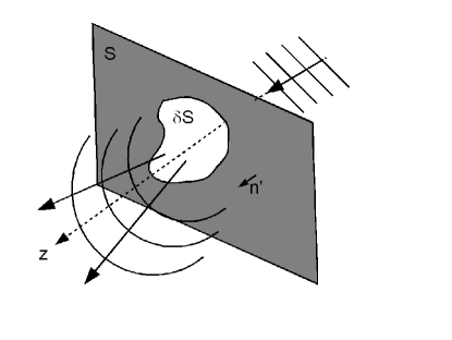
Figure 1:

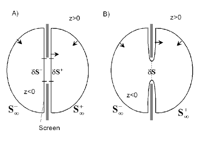
Figure 2:

References

- (1) R. E. Collin, Field Theory of Guided Waves, 2nd ed. (IEEE, Piscataway, NJ, 1991).
- (2) M. Born and E. Wolf, Principles of Optics (Pergamon, Oxford, 1959).
- (3) E. H. Synge, Philos. Mag. 6, 356 (1928).
- (4) D. W. Pohl, W. Denk, and M. Lanz, Appl. Phys. Lett. 44, 651 (1984).
- (5) A. Drezet, J. C. Woehl, and S. Huant, Europhys. Lett. 54, 736 (2001).
- (6) A. Drezet, J. C. Woehl, and S. Huant, Phys. Rev. E 65, 046611 (2002).
- (7) A. Drezet, S. Huant, and J. C. Woehl, Europhys. Lett. 66, 41 (2004).
- (8) H. A. Bethe, Phys. Rev. 66, 163 (1944).
- (9) C. J. Bouwkamp, Philips Res. Rep. 5, 321 (1950).
- (10) C. J. Bouwkamp, Philips Res. Rep.5, 401 (1950).
- (11) W. R. Smythe, Phys. Rev. 72, 1066-1070 (1947).
- (12) W. R. Smythe, Static and Dynamic Electricity (Mc Graw-Hill, New York, 1950).
- (13) C. M. Butler, Y. Rahmat-Samii and R. Mittra, IEEE Trans. Antennas Prop. AP 26, 82 (1978).
- (14) W. H. Eggimann, IRE Trans. Microwave Theory Tech. MTT-9, 408 (1961).
- (15) J. A. Stratton and L. J. Chu, Phys. Rev. 56, 99(1939).
- (16) J. D. Jackson, Classical Electrodynamics (J. Wiley and Sons, New York, 1962).
- (17) J. D. Jackson, Classical Electrodynamics (J. Wiley and Sons, New York, 1975).
- (18) H. Levine and J. schwinger, Phys. Rev. 75, 1423 (1949).
- (19) H. Levine and J. schwinger, Comm. on Pure and Appl. Math. 3 (3), 355 (1950).
- (20) C. Huang, R. SD. Kodis and H. Levine, J. Appl. Phys. 26, 151 (1955).
- (21) H. Poincaré, Théorie mathématique de la lumière (Georges Carré, Paris, 1892).
- (22) Lord Rayleigh, Phil. Mag. 44, 28 (1897).
- (23) A. Sommerfeld, Optics, 3rd ed., (Academic, New York, 1954).
- (24) A. E. H. Love, Philos. Trans. R. Soc. London, serie A 197, 1 (1901).
- (25) J. Larmor, Proc. London Math. Soc. 1, 1 (1903).
- (26) F. Kottler, Ann. Phys. 71, 457 (1923).
- (27) S. A. Schelkunoff, Phys. Rev. 56, 308 (1939).
- (28) S. A. Schelkunoff, Advanced Antenna Theory (Wiley New York , 1952).
- (29) J. A. Stratton, Electromagnetic Theory (Mc Graw-Hill, New York,1947).
- (30) C. J. Bouwkamp, Rep. Prog. Phys. 17, 35 (1954).
- (31) Chen-To Tai, Dyadic Green Functions in Electromagnetic Theory (IEEE, New York, 1994).
- (32) J. Meixner, Ann. Phys. 6, 1 (1949).
- (33) C. Chicanne et al. , Phys. Rev. Lett. 88, 097402 (2002).
- (34) J. C. Weeber et al. , Phys. Rev. E 62, 7381 (2000).
- (35) C. Girard, A. Dereux, C. Joachim, Phys. Rev. E 59, 6097 (2000).
- (36) T. Søndergaard, and S. I. Bozhevolnyi, Phys. Rev. B 69, 045422 (2004).