Entropy and Correlators in Quantum Field Theory

Abstract

It is well known that loss of information about a system, for some observer, leads to an increase in entropy as perceived by this observer. We use this to propose an alternative approach to decoherence in quantum field theory in which the machinery of renormalisation can systematically be implemented: neglecting observationally inaccessible correlators will give rise to an increase in entropy of the system. As an example we calculate the entropy of a general Gaussian state and, assuming the observer’s ability to probe this information experimentally, we also calculate the correction to the Gaussian entropy for two specific non-Gaussian states.

I Introduction

The most natural way of defining the entropy of a quantum system is to use the von Neumann entropy:

$$S_{\rm vN}=-{\rm Tr}[\hat{\rho}\ln(\hat{\rho})]\,,$$ (1)

where $\hat{\rho}$ denotes the density operator which in the Schrödinger picture satisfies the von Neumann equation:

$$\imath\hbar\frac{\partial}{\partial t}\hat{\rho}=[\hat{H},\hat{\rho}]\,,$$ (2)

where $\hat{H}$ is the Hamiltonian. Since quantum mechanics and quantum field theory are unitary theories, the von Neumann entropy is conserved, albeit in general not zero.

The decoherence program Zeh:1970 ; Joos:1984uk usually assumes the existence of some environment that is barely observable to some observer. This allows us to construct a reduced density operator $\hat{\rho}_{\mathrm{red}}$ characterising the system S, which is obtained by tracing over the unobservable environmental degrees of freedom E: $\hat{\rho}_{\mathrm{red}}={\rm Tr}_{E}[\hat{\rho}]$. This is a non-unitary process which consequently generates entropy. This operation is justified by the observer’s inability to see the environmental degrees of freedom (or better: access the information stored in the ES-correlators). Yet, tracing out some degrees of freedom results in complications. The simple looking von Neumann equation (2) is replaced by an equation for the reduced density operator. This “master equation” PazZurek:2001 ; Zurek:2003zz can be solved for only in very simple situations, which has hampered progress in decoherence studies in the context of interacting quantum field theories. In particular, we are not aware of any known solution of the master equation that would include perturbative corrections and implement the program of renormalisation. Also, one has no control of the error in a calculation in the perturbative sense induced by neglecting non-Gaussian corrections.

Here we propose a decoherence program that can be implemented in a field theoretical setting and that also allows us to incorporate renormalisation procedures. The idea is very simple, and we present it for a real scalar field $\phi(x)$. A generalisation to other types of fields, e.g. gauge and fermionic fields, should be quite straightforward.

The density matrix $\hat{\rho}(t)$ contains all information about the (possibly mixed) state a quantum system is in. From the density matrix one can, in principle, calculate various correlators. For example, the three Gaussian correlators are given by:

$$\langle\hat{\phi}(\vec{x})\hat{\phi}(\vec{y})\rangle = {\rm Tr}[\hat{\rho}(t)\hat{\phi}(\vec{x})\hat{\phi}(\vec{y})]=F(\vec{x},t;\vec{y},t^{\prime})|_{t=t^{\prime}}$$ (3a)

$$\langle\hat{\pi}(\vec{x})\hat{\pi}(\vec{y})\rangle = {\rm Tr}[\hat{\rho}(t)\hat{\pi}(\vec{x})\hat{\pi}(\vec{y})]=\partial_{t}\partial_{t^{\prime}}F(\vec{x},t;\vec{y},t^{\prime})|_{t=t^{\prime}}$$ (3b)

$$\frac{1}{2}\langle\{\hat{\phi}(\vec{x}),\hat{\pi}(\vec{y})\}\rangle = \frac{1}{2}{\rm Tr}[\hat{\rho}(t)\{\hat{\phi}(\vec{x}),\hat{\pi}(\vec{y})\}]=\partial_{t^{\prime}}F(\vec{x},t;\vec{y},t^{\prime})|_{t=t^{\prime}}\,,$$ (3c)

where $\hat{\pi}$ denotes the momentum field conjugate to $\hat{\phi}$, and where the curly brackets denote the anti-commutator as usual. Note that these three Gaussian correlators can all be determined from the statistical propagator $F(\vec{x},t;\vec{y},t^{\prime})$ in the Heisenberg picture as usual in quantum field theory. The fourth Gaussian correlator is trivial as it is restricted by the canonical commutation relations. There is an infinite number of higher order, non-Gaussian correlators that characterise a system, where one can think of e.g.:

$$\langle\hat{\phi}(\vec{x}_{1})\cdots\hat{\phi}(\vec{x}_{n})\rangle = {\rm Tr}[\hat{\rho}(t)\hat{\phi}(\vec{x}_{1})\cdots\hat{\phi}(\vec{x}_{n})]$$ (4a)

$$\langle\hat{\pi}(\vec{x}_{1})\cdots\hat{\pi}(\vec{x}_{n})\rangle = {\rm Tr}[\hat{\rho}(t)\hat{\pi}(\vec{x}_{1})\cdots\hat{\pi}(\vec{x}_{n})]\,,$$ (4b)

where $$n\geq 3 \hat{\phi} \hat{\pi}$$. Moreover, one can also imagine a higher order correlation function consisting of a mixture of both ’s and ’s. Finally, one could think of other non-Gaussian correlators obtained by further differentiating the statistical propagator:

$$\partial_{t}^{n}\partial_{t^{\prime}}^{m}F(\vec{x},t;\vec{y},t^{\prime})|_{t=t^{\prime}}=\partial_{t}^{n}\partial_{t^{\prime}}^{m}{\rm Tr}[\hat{\rho}(t_{0})\hat{\phi}(\vec{x},t)\hat{\phi}(\vec{y},t^{\prime})]|_{t=t^{\prime}}\,,$$ (4c)

where $n+m\geq 3$. For free theories, all the non-Gaussian correlators either vanish or can be expressed in terms of the Gaussian correlators.

Let us turn our attention to interacting field theories and present two simple arguments why, generally speaking, the Gaussian correlators dominate over the non-Gaussian correlators. In interacting quantum field theories, the Gaussian correlators all stem from tree-level physics, whereas non-Gaussian correlators are generated by the interactions. Relying on a perturbative treatment of these interactions, we can safely expect that all of these higher order, non-Gaussian correlators above are suppressed as they generically are proportional to a non-zero power of the (perturbatively small) interaction coefficient. A second, more heuristic, argument invokes the (classical) central limit theorem, according to which systems with many stochastic mutually independent degrees of freedom tend to become normally distributed, and hence nearly Gaussian. While this theorem is derived for classical systems and for independent stochastic variables, we believe that it will in a certain quantum disguise also apply to weakly interacting quantum systems with many degrees of freedom.

Hence, we expect that to a good approximation, many of the relevant properties of quantum systems are encoded in the Gaussian part $\hat{\rho}_{\rm{g}}$ of the density operator $\hat{\rho}$ and the non-Gaussian correlators are thus typically much more difficult to access. The crucial point is that all information about a general Gaussian density matrix and thus about the Gaussian part of a state, is stored only in the three equal time correlators (3). All non-Gaussian correlators like (4) contain information about the correlations between the system and environment as well as the environment’s correlations induced by higher order interactions. When projected on the field amplitude basis in the Schrödinger picture, the Gaussian part of a density matrix reads:

$$\rho_{\mathrm{g}}[\phi,\phi^{\prime};t]\equiv\langle\phi|\hat{\rho}_{\mathrm{g}}(t)|\phi^{\prime}\rangle={\cal N}\exp\!\left[\!-\!\int\!\mathrm{d}^{3}x\mathrm{d}^{3}y\left(\phi(\vec{x}\,)A(\vec{x},\vec{y};t)\phi(\vec{y}\,)+\phi^{\prime}(\vec{x}\,)B(\vec{x},\vec{y};t)\phi^{\prime}(\vec{y}\,)-2\phi(\vec{x}\,)C(\vec{x},\vec{y};t)\phi^{\prime}(\vec{y}\,)\right)\right]\!,$$ (5)

where $A,B,C$ and ${\cal N}$ are functions of the equal time field correlators (for details see sections V). Of course, the von Neumann equation (2) does not hold any more for $\hat{\rho}_{\rm g}$, and thus the entropy conservation law is violated by $\hat{\rho}_{\rm g}$. Indeed, neglecting the information stored in observationally inaccessible correlators will give rise to an increase of the entropy.

The purpose of the present work is to calculate the entropy of a system taking these considerations into account. We distinguish two cases. In the simplest case we assume that our observer can only measure Gaussian correlators and his apparatus is insensitive to all non-Gaussian correlators. We will consider this situation in sections II and III. In quantum field theories, the problem seems to be that the evolution equations of the three Gaussian correlators (3) do not close as soon as perturbative corrections are included. The reason is that off-shell physics becomes important. A way out of this impasse, and in our opinion the way out, is to solve for the dynamics of the unequal time statistical correlator, i.e. the statistical propagator, from which one then extracts the three relevant correlators (3).

In the second case, we assume that our observer is sensitive to specific types of non-Gaussianities present in our theory, apart from the leading order Gaussian correlators of course, either because the observer has developed a sensitive measurement device or the non-Gaussianities happen to be large enough. We will consider this case in section IV. The sections above contain, for pedagogical reasons, quantum mechanical derivations rather than quantum field theoretical calculations. We will generalise our results to quantum field theory in section V.

This paper aims only at developing the necessary machinery to discuss entropy generation in an interacting quantum field theory in an out-of-equilibrium setting, see e.g. Chou:1984es ; Jordan:1986ug ; Calzetta:1986cq ; Aarts:2001qa ; Aarts:2001yn ; Aarts:2002dj ; Berges:2002cz ; Juchem:2003bi ; Juchem:2004cs ; Berges:2004yj . We discuss the application of these ideas elsewhere Koksma:2009wa ; Koksma:2010 in great detail, where we consider a scalar field $\phi$ coupled to a second scalar field via the interaction Lagrangian density ${\cal L}_{\rm int}=-\frac{1}{2}h\chi^{2}(x)\phi(x)$. The results we develop here are applicable to a much more wider class of field theoretical models, including gauge and fermionic fields.

II Gaussian Entropy from the Wigner Function

Entropy has of course been widely studied over the years Wehrl:1978zz ; Mackey:1989zz ; Barnett:1991zz ; Serafini:2003ke ; Cacciatori:2008qs ; Adesso:2007jg . In this section we will derive an entropy formula based on a naïve probabilistic interpretation of the Wigner function. This characterises much of the 20th century efforts to connect the Wigner function, Boltzmann’s equations, Boltzmann’s H-theorem and macroscopic entropy Hillery:1983ms . Let us begin by considering the Hamiltonian of a time dependent harmonic oscillator, which is the one-particle “free” Hamiltonian:

$$H(p,x)=\frac{p^{2}}{2m}+\frac{1}{2}m\omega^{2}x^{2}+H_{\mathrm{s}}\,,\qquad H_{\mathrm{s}}=xj\,.$$ (6)

In general, the oscillator’s mass and frequency and the source current can all depend on time: $m=m(t)$, $\omega=\omega(t)$ and $j=j(t)$, respectively. $H_{\mathrm{s}}$ is the source Hamiltonian and $j=j(t)$ the corresponding current. This Hamiltonian is relevant both for many condensed matter systems that can be realised in laboratories and in an early Universe setting. For the latter, the time dependence of the parameters is introduced for example by the Universe’s expansion or by phase transitions. Alternatively, this Hamiltonian can represent for example the simplest model of a laser, where $x=x(t)$ is the photon amplitude, where, if $m\rightarrow 1$, $\omega(t)\rightarrow E(t)/\hbar$ is the photon’s frequency and where $j=j(t)$ is a charge current that coherently pumps energy into the system, transforming the vacuum state into a coherent state Glauber:1963tx ; Cahill:1969iq .

The time dependence of the parameters changes the system’s energy, but simultaneously does not change the Gaussian nature of a state if such a state is imposed initially, i.e.: the evolution implied by the Hamiltonian (6) transforms an initial Gaussian density matrix into another Gaussian density matrix. Moreover, as we will come to appreciate, one has to add a coupling to the environment or add a self-interaction to generate entropy. The Lagrangian $L=p\dot{x}-H$ follows as usual from the Hamiltonian. Note that the source term can be removed from this Lagrangian by a simple coordinate shift:

$$x(t)\rightarrow z(t)=x(t)-x_{0}(t)\,,$$ (7)

upon which the Lagrangian reduces to a quadratic form:

$$L=\frac{1}{2}m\dot{z}^{2}-\frac{1}{2}m\omega^{2}z^{2}+L_{0}(t)+\frac{\mathrm{d}}{\mathrm{d}t}\left[mz\dot{x}_{0}\right]\,.$$ (8)

Here, $L_{0}(t)$ is a $z$-independent function of time and the last term is a boundary term which does not contribute to the equation of motion if $x_{0}(t)$ is a function that obeys:

$$\frac{\mathrm{d}}{\mathrm{d}t}\left[m\dot{x}_{0}\right]+m\omega^{2}x_{0}+j=0\,.$$ (9)

A general Gaussian density matrix centered at the new origin remains a Gaussian density matrix centered at the origin under the evolution of a quadratic Hamiltonian and moreover, which is what the analysis above shows, linear source terms in the Hamiltonian will not alter the Gaussian nature of the state. We can thus consider Gaussian density matrices centered at the origin, whose time evolution is governed by an Hamiltonian of the form (6) with $j(t)\rightarrow 0$. When written in position space representation, the single particle density operator of a quantum mechanical Gaussian state centered at the origin is of the form:

$$\hat{\rho}_{\mathrm{g}}(t)=\int_{-\infty}^{\infty}\mathrm{d}x\int_{-\infty}^{\infty}\mathrm{d}y|x\rangle\rho_{\mathrm{g}}(x,y;t)\langle y|\,,$$ (10a)

where:

$$\rho_{\mathrm{g}}(x,y;t)={\cal N}(t)\exp\left[-a(t)x^{2}-b(t)y^{2}+2c(t)xy\right]\,,$$ (10b)

and where $a=a(t)$, $b=b(t)$ and $c=c(t)$ are determined from the von Neumann equation (2). The subscript g denotes “Gaussian”. Moreover, from $\hat{\rho}_{\mathrm{g}}^{\dagger}=\hat{\rho}_{\mathrm{g}}$ it follows that $b^{*}=a$ and $c^{*}=c$. When $c=0$ one recovers a pure state with vanishing entropy. However when $c\neq 0$ the density matrix is mixed and entangled and it cannot be written in the simple diagonal form, $\rho_{\mathrm{g}}(x,y;t)=\Psi^{*}(y,t)\Psi(x,t)$, where $\Psi(x,t)=\sqrt{{\cal N}}\exp(-ax^{2})$. When $c>0$ the density matrix tends to get diagonal in the $x-y$ direction, however when $c<0$ the diagonalisation occurs in the $x+y$ direction in which case the entropy is not defined. The Heisenberg uncertainty relation is in trouble in this case as we will see in equation (30). Hence it is natural to assume that $c>0$. We keep the discussion phenomenological and do not discuss the physical origin of $c\neq 0$. The normalisation ${\cal N}$ is obtained from requiring $\mathrm{Tr}[\hat{\rho}_{\mathrm{g}}]=1$:

$$\mathrm{Tr}[\hat{\rho}_{\mathrm{g}}]=\int_{-\infty}^{\infty}\mathrm{d}\tilde{x}\langle\tilde{x}|\hat{\rho}_{\mathrm{g}}|\tilde{x}\rangle=\int_{-\infty}^{\infty}\mathrm{d}x\rho_{\mathrm{g}}(x,x;t)={\cal N}\sqrt{\frac{\pi}{2(a_{\mathrm{R}}-c)}}=1\,,$$ (11)

from which we conclude:

$${\cal N}=\sqrt{\frac{2(a_{\mathrm{R}}-c)}{\pi}}\,,$$ (12)

provided that $c<a_{\mathrm{R}}$ where $a_{\mathrm{R}}=\Re[a]$. The equations that the functions $a(t)$, $b(t)$ and $c(t)$ of the density matrix (10b) obey can easily be obtained from the von Neumann equation (2), which in this Gaussian case in the amplitude basis reads:

$$\imath\hbar\partial_{t}\rho_{\mathrm{g}}(x,y;t)=-\frac{\hbar^{2}}{2m}\left(\partial^{2}_{x}-\partial^{2}_{y}\right)\rho_{\mathrm{g}}(x,y;t)+\frac{1}{2}m\omega^{2}(x^{2}-y^{2})\rho_{\mathrm{g}}(x,y;t)\,.$$ (13)

If we insert equation (10b) in the equation above we find:

$$\frac{\mathrm{d}a_{\mathrm{R}}}{\mathrm{d}t} = \frac{4\hbar}{m}a_{\mathrm{I}}a_{\mathrm{R}}$$ (14a)

$$\frac{\mathrm{d}c}{\mathrm{d}t} = \frac{4\hbar}{m}a_{\mathrm{I}}c$$ (14b)

$$\frac{\mathrm{d}}{\mathrm{d}t}\ln({\cal N}) = \frac{2\hbar}{m}a_{\mathrm{I}}$$ (14c)

$$\frac{\mathrm{d}a_{\mathrm{I}}}{\mathrm{d}t} = \frac{2\hbar}{m}\left(a_{\mathrm{I}}^{2}-a_{\mathrm{R}}^{2}+c^{2}\right)+\frac{m\omega^{2}}{2\hbar}\,,$$ (14d)

where we defined $a_{\mathrm{I}}=\Im[a]$. Note that ${\cal N}\propto\sqrt{a_{\mathrm{R}}-c}$ is consistent with equation (14c) as it should.

The Wigner function is defined as a Wigner transform of the density matrix $\rho_{\mathrm{g}}(x,y;t)$:

$${\cal W}(q,p;t)=\int_{-\infty}^{\infty}\mathrm{d}r{\rm e}^{-\imath pr/\hbar}\rho_{\mathrm{g}}(q+r/2,q-r/2;t)\,,$$ (15)

where we defined the average and relative coordinates, $q=(x+y)/2$ and $r=x-y$, respectively. Hence, a Wigner transform can be thought of as an ordinary Fourier transform with respect to the relative coordinate $r$ of the density matrix. The inverse Wigner transform determines $\rho_{\mathrm{g}}(x,y;t)$ in terms of ${\cal W}(q,p;t)$:

$$\rho_{\mathrm{g}}(x,y;t)=\int_{-\infty}^{\infty}\frac{\mathrm{d}p}{2\pi\hbar}{\rm e}^{\imath p(x-y)/\hbar}{\cal W}(q,p;t)\,,$$ (16)

where $2\pi\hbar$ is the standard phase space measure. We obtain the Gaussian Wigner function by performing the integral (15):

$${\cal W}(q,p;t)={\cal M}(t)\exp\left[-\alpha_{\mathrm{w}}(t)q^{2}-\beta_{\mathrm{w}}(t)(p+qp_{\mathrm{c}}(t))^{2}\right]\,,$$ (17)

where:

$$\alpha_{\mathrm{w}} = 2(a_{\mathrm{R}}-c)$$ (18a)

$$\beta_{\mathrm{w}} = \frac{1}{2\hbar^{2}(a_{\mathrm{R}}+c)}$$ (18b)

$$p_{\mathrm{c}} = 2\hbar a_{\mathrm{I}}$$ (18c)

$${\cal M} = \sqrt{\frac{4(a_{\mathrm{R}}-c)}{a_{\mathrm{R}}+c}}\,,$$ (18d)

and $p_{\mathrm{c}}$ denotes a “classical” momentum, which makes the Wigner function non-diagonal. Note that the Wigner function (17) is normalised to unity, in the sense that:

$$\int_{-\infty}^{\infty}\frac{\mathrm{d}q\mathrm{d}p}{2\pi\hbar}{\cal W}(q,p;t)=1\,.$$ (19)

Recalling definition (15), equation (13) transforms to:

$$\Big{(}\partial_{t}+\frac{p}{m}\partial_{q}-m\omega^{2}q\partial_{p}\Big{)}{\cal W}(q,p;t)=0\,,$$ (20)

where we made use of the following relations:

$$\left(\partial_{x}^{2}-\partial_{y}^{2}\right)\rho_{\mathrm{g}}(x,y;t) = 2\partial_{q}\partial_{r}\rho_{\mathrm{g}}(q+r/2,q-r/2;t)$$ (21a)

$$r\mathrm{e}^{\imath pr/\hbar} = -\imath\hbar\partial_{p}\mathrm{e}^{\imath pr/\hbar}\,.$$ (21b)

Upon noting that $p/m=\dot{x}=\partial_{p}H$ and $-m\omega^{2}x=\dot{p}=-\partial_{x}H$, we see that equation (20) is nothing but the Liouville equation for the Boltzmann’s distribution function $f(x,p;t)$,

$$\partial_{t}f(x,p;t)+\dot{x}\partial_{x}f(x,p;t)+\dot{p}\partial_{p}f(x,p;t)=0\,.$$ (22)

A probabilistic interpretation of the Wigner function thus seems plausible by the following identification:

$${\cal W}(q,p;t)\Leftrightarrow f(x,p;t)\,.$$ (23)

Of course, the equations for ${\cal W}(q,p;t)$ and $f(x,p;t)$ are identical only in a free harmonic oscillator theory and, when interactions are included, differences arise between the von Neumann equation for the density operator $\hat{\rho}_{\mathrm{g}}(t)$ (or the corresponding equation for ${\cal W}(q,p;t)$) and the Boltzmann equation for $f(x,p;t)$. This indeed makes the identification (23) less rigorous but it remains a useful picture. The correspondence (23) has been widely used in the literature to develop a formalism relevant for example for the physics of heavy ion collisions Mrowczynski:1992hq ; Aarts:2002dj or for baryogenesis Prokopec:2003pj ; Prokopec:2004ic .

In the distant 1969 Cahill and Glauber Cahill:1969iq have proposed to approximate the density operator in the coherent state basis $|\alpha\rangle$ by its diagonal form: $\rho_{\mathrm{g}}\approx\rho_{\rm cs}(\alpha)=\langle\alpha|\hat{\rho}_{\mathrm{g}}|\alpha\rangle$, which they interpret as a quasi-probability distribution. Since coherent states harbour many properties of classical particles, one can argue that this is reasonable. Recall that coherent states are defined by $\hat{a}|\alpha\rangle=\alpha|\alpha\rangle$, where $\hat{a}=\sqrt{m\omega/2}[\hat{x}+\imath\hat{p}/(m\omega)]$ denotes the annihilation operator for the oscillator (6). The density matrix $\rho_{\rm cs}(\alpha)$ represents an early example of a quasi-probability distribution for a quantum system. Needless to say, by this line of reasoning one can get only approximate answers for the expectation value $\langle\hat{A}\rangle={\rm Tr}[\hat{\rho}_{\mathrm{g}}\hat{A}]$ of an operator $\hat{A}$ and likewise for the entropy (which is just the expectation value of $-\ln(\hat{\rho}_{\mathrm{g}})$). Another common way of approximating expectation values of operators is to give a probabilistic interpretation to the Wigner function, along the same line of reasoning as argued above in equation (23) for a free theory. In this approach Cahill:1969iq ; Brandenberger:1992jh the entropy is approximated by:

$$S\approx S_{\cal W}\equiv-{\rm Tr}[{\cal W}(q,p;t)\ln({\cal W}(q,p;t))]\,,$$ (24)

where the trace ${\rm Tr}\rightarrow\int\mathrm{d}p\mathrm{d}q/[2\pi\hbar]$ should be interpreted as an integration over the phase space volume as in equation (19). We now insert (17) into (24) to find:

$$S_{\cal W} = \frac{1}{2}\ln\left(\frac{a_{\mathrm{R}}+c}{a_{\mathrm{R}}-c}\right)+1-\ln(2)$$ (25)

$$= \ln\left(\frac{\Delta}{2}\right)+1\,,$$

where we defined:

$$\Delta^{2}=\frac{a_{\mathrm{R}}+c}{a_{\mathrm{R}}-c}\,.$$ (26)

We evaluated the phase space Gaussian integrals by shifting the momentum integration to $p^{\prime}=p-p_{c}$ (the Jacobian of this shift equals unity). At this point, it is useful to evaluate a few quantum mechanical expectation values. We can extract the following correlators from our Gaussian state:

$$\langle\hat{x}^{2}\rangle = {\rm Tr}[\hat{\rho}_{\mathrm{g}}\hat{x}^{2}]=\int_{-\infty}^{\infty}\mathrm{d}\tilde{x}\langle\tilde{x}|\hat{\rho}_{\mathrm{g}}\hat{x}^{2}|\tilde{x}\rangle=\frac{1}{4(a_{\mathrm{R}}-c)}$$ (27a)

$$\Big{\langle}\frac{1}{2}\{\hat{x},\hat{p}\}\Big{\rangle} = -\hbar\frac{a_{\mathrm{I}}}{2(a_{\mathrm{R}}-c)}$$ (27b)

$$\langle\hat{p}^{2}\rangle = \hbar^{2}\frac{|a|^{2}-c^{2}}{a_{\mathrm{R}}-c}\,.$$ (27c)

Here, we made use of $\langle x|\hat{p}|\psi\rangle=-\imath\hbar\partial_{x}\langle x|\psi\rangle$. Moreover, one can easily verify that $\langle[\hat{x},\hat{p}]\rangle=\langle\hat{x}\hat{p}-\hat{p}\hat{x}\rangle=\imath\hbar$ as it should. This enables us to find the equivalent inverse relations:

$$a_{\mathrm{I}} = -\frac{\left\langle\frac{1}{2}\{\hat{x},\hat{p}\}\right\rangle}{2\hbar\langle\hat{x}^{2}\rangle}$$ (28a)

$$a_{\mathrm{R}} = \frac{\Delta^{2}+1}{8\langle\hat{x}^{2}\rangle}$$ (28b)

$$c = \frac{\Delta^{2}-1}{8\langle\hat{x}^{2}\rangle}\,,$$ (28c)

and to express $\Delta(t)$ in equation (26) in terms of the correlators (27):

$$\Delta^{2}(t)=\frac{4}{\hbar^{2}}\left[\langle\hat{x}^{2}\rangle\langle\hat{p}^{2}\rangle-\Big{\langle}\frac{1}{2}\{\hat{x},\hat{p}\}\Big{\rangle}^{2}\right]\,.$$ (29)

For the moment this is just a definition, but as we will come to discuss, the physical meaning of $\hbar\Delta(t)$ is the phase space area in units of $\hbar$ occupied by a (Gaussian) state centered at the origin. For a pure state $\Delta(t)=1$, while for a mixed state $\Delta(t)>1$. Hence, we can define the uncertainty relation for a general Gaussian state:

$$\frac{(\hbar\Delta(t))^{2}}{4}=\langle\hat{x}^{2}\rangle\langle\hat{p}^{2}\rangle-\Big{\langle}\frac{1}{2}\{\hat{x},\hat{p}\}\Big{\rangle}^{2}\geq\frac{\hbar^{2}}{4}\,.$$ (30)

If $c$ is negative and $|c|<a_{\mathrm{R}}$, we can in principle have $\Delta<1$, which can be seen from equation (26). It would be interesting to investigate whether any physical experiment could be proposed where a violation of Heisenberg’s uncertainty relation occurs, even if it were for only a very brief moment in time (such that it would still hold on average).

Furthermore, it is natural to define the statistical particle number density on our phase space, in the quantum field theoretical sense, as:

$$n(t)\equiv\frac{\Delta(t)-1}{2}\,,$$ (31)

in terms of which the Wigner entropy (25) can be rewritten as:

$$S_{\cal W}(t)=\ln\left(n(t)+\frac{1}{2}\right)+1\,.$$ (32)

These results in essence agree with the entropy per mode of scalar cosmological perturbations obtained in Brandenberger:1992jh . Shortly we shall see that the Wigner entropy (32) is a good approximation for the von Neumann entropy if $n\gg 1$, or equivalently when $\hbar\Delta\gg 1$.

Let us try to put these results briefly in historical context. The fundamental question that is left unanswered in Brandenberger:1992jh is what the dynamical mechanism for the growth of $\Delta$ is. Instead, the authors argue that an observer that measures cosmological perturbations can be approximated by a coherent state (which is a good classical basis), thus explaining the growth in $\Delta$. Two mechanisms were considered in Prokopec:1992ia : a projection on the particle number basis and on the coherent state basis. In both cases, information of the phase of the squeezed Gaussian state is lost, which thus generates entropy. In the latter approach formula (29) is reproduced, while in the former, the entropy acquires the form of the statistical entropy of Bose particles $S=(n+1)\ln(n+1)-n\ln(n)$ with $n\rightarrow\sinh^{2}(r)$ the particle number associated with the squeezed state, and $r$ the squeezing parameter of the state. While these early articles, and many subsequent ones Polarski:1995jg ; Kiefer:1999sj , attempted to explain the origin of entropy of cosmological perturbations by a (non-unitary) process of coarse graining (associated with particular properties of the observer’s measuring apparatus), a genuine dynamical mechanism of entropy generation was lacking.

This has changed recently Campo:2004sz ; Campo:2005sy ; Prokopec:2006fc ; Kiefer:2006je ; Kiefer:2007zza ; Campo:2008ju ; Campo:2008ij ; Koksma:2009wa , now dynamical mechanisms for entropy generation have been proposed. Rather than discussing various mechanisms in detail, let us just point out that the notion of how entropy should be defined and generated has evolved: recently, it has been advocated that the relevant entropy to consider is the Gaussian entropy, although the approaches differ in the actual origin of the entropy increase. For example, Prokopec and Rigopoulos suggested in Prokopec:2006fc that tracing over the unobserved isocurvature perturbations leads to entropy generation in the adiabatic mode. Similarly, tracing over the unobserved gravitational waves should lead to entropy generation in the adiabatic mode Koksma:2007zz . Kiefer, Lohmar, Polarski and Starobinsky Kiefer:2006je ; Kiefer:2007zza as well as Campo and Parentani Campo:2008ju ; Campo:2008ij , among others, suggested that, if super-Hubble modes take the role of the system, the origin of the entropy of cosmological perturbations should be associated with the stochastic noise generated by the sub-Hubble ultraviolet modes representing the environment. Both Giraud and Serrau Giraud:2009tn and we Koksma:Talk ; Koksma:Talk2 ; Koksma:2009wa advocate that neglecting observationally inaccessible non-Gaussianities is a prominent mechanism to generate entropy.

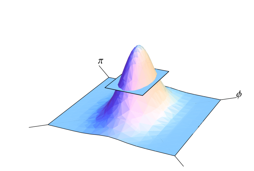
Figure 1: General shape of the Wigner function, representing the 2-dimensional Gaussian phase space distribution of a certain state. The $1\sigma$ or $2\sigma$ cross-section is an ellipse. For the current quantum mechanical discussion, we of course let $\pi\rightarrow p$ and $\phi\rightarrow q$.

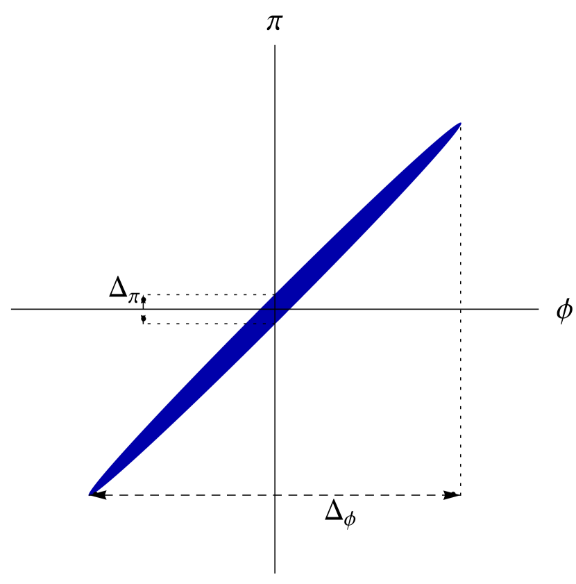
Figure 2: Squeezed state before decoherence. For example, the area of the ellipse of a vacuum state would be unity $\Delta=1$. For the current quantum mechanical discussion, we of course let $\pi\rightarrow p$ and $\phi\rightarrow q$, also in figure 3.

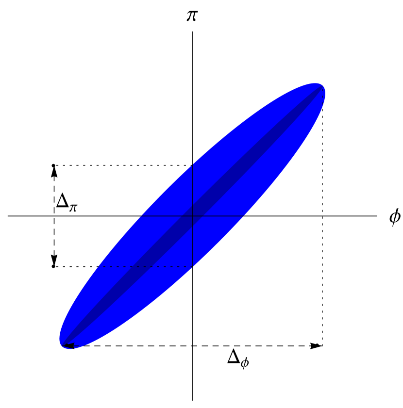
Figure 3: Squeezed state after decoherence. Clearly, the accessible phase space has increased and one can say that knowledge about the system has been lost. The entropy has increased compared to figure 3.

So far, we have discussed how the Gaussian entropy in Wigner space is defined and qualitatively discussed various mechanisms to generate entropy dynamically. Let us now, to finish this section, discuss how one can sensibly think of a decohered state in Wigner space and discuss the physical meaning of $\Delta(t)$. Despite the fact that the Wigner entropy (25) only approximates the von Neumann entropy, it offers a useful, intuitive way of depicting decohered states irrespective of the precise underlying mechanism by which such a state has decohered in the first place. Let us, for this reason, discuss this phenomenologically. The Wigner function (17) is a 2-dimensional Gaussian function whose width in the $p$-direction need a priori not necessarily be the same as in the $q$-direction. Hence, in general it can be squeezed in some direction. This is illustrated in figure 3. The $1\sigma$ or $2\sigma$ cross-section of the phase space distribution has the shape of an ellipse, which we also visualised in figure 3. If the cross-section is a circle centered at the origin, the state is either pure or mixed and if, moreover, its area is unity $\Delta(t)=1$ it is a pure vacuum state. If the cross-section is again a circle but displaced from the origin, we are dealing with a generalised coherent-squeezed state (whose shape is not described by equation (25) for obvious reasons). If the cross-section is an ellipse, it is a squeezed state as mentioned before. The ellipse is parametrised by:

$$\alpha_{\mathrm{w}}(t)q^{2}+\beta_{\mathrm{w}}(t)\left(p+q\,p_{\mathrm{c}}(t)\right)^{2}=\vartheta\,,$$ (33)

where we have made use of equation (17) and where $\vartheta$ is some constant that determines the height at which we slice the Wigner function. The area of this ellipse is now given by:

$$\mathcal{A}(t)=\frac{\vartheta\pi}{\sqrt{\alpha_{\mathrm{w}}(t)\beta_{\mathrm{w}}(t)}}=\vartheta\pi\hbar\Delta(t)\,,$$ (34)

where we have used equations (18) and (26). Clearly, the area of the ellipse in Wigner space is determined straightforwardly from the phase space area $\Delta(t)$. Note that if $\vartheta=1/\pi$ we have $\mathcal{A}=\Delta$.

Figures 3 and 3 visualise the decoherence process of a squeezed state. Initially, in figure 3, the state is squeezed and has unity phase space area $\Delta(t_{0})=1$, such that its entropy vanishes. Now we switch on our favourite decoherence mechanism: the state interacts with some environment and environmental degrees of freedom are traced over or non-Gaussian correlators generated by the interaction with the environment are neglected. Consequently, the area in phase space increases $\Delta(t)>1$, such that $S(t)>0$. Hence, the ellipse in Wigner space grows which we depict in figure 3. An important feature of any decoherence process reveals itself: for a highly squeezed state, given the knowledge of $q$ after some measurement, the value $p$ can take in a subsequent measurement is constraint in a very narrow interval. Interestingly, after the state has decohered, and given the same measurement of $q$, the range of values $p$ can take has increased. Indeed one can say that knowledge about $p$ has been lost compared to the squeezed state before decoherence, hence entropy has been generated. Alternatively, we can say that given some measurement of $q$, the value $p$ can take is, after decoherence, drawn from a classical stochastic distribution, which indeed coincides with the familiar idea that decohered quantum systems should behave as uncorrelated stochastic systems. Indeed, $n$ roughly counts the number of patches in phase space that behave independently and are uncorrelated.

With this intuitive notion of decohered state in mind, one can understand that, for highly squeezed states, the position space basis (which generalises to the field amplitude basis in the quantum field theoretical case) is the pointer basis. Let us start out with a highly squeezed state, i.e.: take for example a pure state during inflation that rapidly squeezes during the Universe’s expansion. The Hamiltonian of the state is then dominated by the potential term, and the kinetic term only contributes little. In thermal equilibrium, the system will minimise its free energy $F=H-TS$, where $T$ is the temperature of the heat bath. Now, if we switch on some decoherence mechanism due to interaction with the environment, the entropy will increase mainly due to momentum increase, i.e.: $\langle\hat{p}^{2}\rangle$ will increase. Indeed, increasing $\langle\hat{p}^{2}\rangle$ will hardly affect the Hamiltonian, whereas it will significantly affect the entropy. Hence, the variable $x$ is robust during the process of decoherence, in the sense that $\langle\hat{x}^{2}\rangle$ will hardly change such that it qualifies as a proper pointer basis. Note however, that $x$ is only a pointer basis in the statistical sense, such that there is a well defined probability distribution function from which a measurement can be drawn.

III Gaussian entropy from the replica trick

The entropy of a general Gaussian state has been derived by Sohma, Holevo and Hirota SohmaHolevoHirota:1999 ; SohmaHolevoHirota:2000 by making use of Glauber’s P representation for the density operator. Here we present an alternative derivation for the von Neumann entropy (1) of a general Gaussian state by making use of the replica trick (see e.g.: Callan:1994py ; Calabrese:2009qy ; Calabrese:2004eu ). Of course, there are other analogous methods one can use. Notice first that:

$$\ln(\hat{\rho}_{\mathrm{g}})=\lim_{\epsilon\rightarrow 0}\frac{\hat{\rho}_{\mathrm{g}}^{\epsilon}-1}{\epsilon}\,.$$ (35)

Here, $\epsilon$ is a positive integer which is analytically extended to zero. Hence, in order to calculate the entropy (1) we need to evaluate ${\rm Tr}\left[\hat{\rho}_{\mathrm{g}}^{1+\epsilon}\right]$. Using equation (10), we thus have:

$${\rm Tr}\left[\hat{\rho}_{\mathrm{g}}^{1+\epsilon}\right] = {\cal N}^{1+\epsilon}\int_{-\infty}^{\infty}\mathrm{d}x_{0}\cdots\int_{-\infty}^{\infty}\mathrm{d}x_{\epsilon}\exp\left[-2a_{\mathrm{R}}\left(x_{0}^{2}+\cdots+x_{\epsilon}^{2}\right)+2c\left(x_{0}x_{1}+x_{1}x_{2}+\cdots+x_{\epsilon}x_{0}\right)\right]$$ (36)

$$= {\cal N}^{1+\epsilon}\int_{-\infty}^{\infty}\mathrm{d}x_{0}\cdots\int_{-\infty}^{\infty}\mathrm{d}x_{\epsilon}\exp\left[-2\beta\left\{(x_{0}-\alpha x_{1})^{2}+(x_{1}-\alpha x_{2})^{2}+\cdots+(x_{\epsilon}-\alpha x_{0})^{2}\right\}\right]$$

$$= |1-\alpha^{1+\epsilon}|^{-1}\left({\cal N}\int_{-\infty}^{\infty}\mathrm{d}y\exp\left[-2\beta y^{2}\right]\right)^{1+\epsilon}$$

$$= |1-\alpha^{1+\epsilon}|^{-1}\left(\frac{a_{\mathrm{R}}-c}{\beta}\right)^{\frac{1+\epsilon}{2}}\,.$$

Here, $J=|1-\alpha^{1+\epsilon}|^{-1}$ is the Jacobian of the transformation from $x_{i}$ to $y_{i}=x_{i}-\alpha x_{i+1}$, where $i=\{0,1,\cdots,\epsilon-1\}$, and $y_{\epsilon}=x_{\epsilon}-\alpha x_{0}$. A comparison of the first and the second line in (36) tells us that:

$$\alpha_{\pm} = \frac{a_{\mathrm{R}}}{c}\pm\sqrt{\left(\frac{a_{\mathrm{R}}}{c}\right)^{2}-1}$$ (37a)

$$\beta_{\pm} = \frac{c}{2\alpha_{\pm}}=\frac{c\alpha_{\mp}}{2}\,.$$ (37b)

In the limit $c\rightarrow 0$ one must recover a pure diagonal density operator and, consequently, the shift $\alpha$ should vanish, singling out:

$$\alpha = \alpha_{-}=\frac{a_{\mathrm{R}}}{c}-\sqrt{\left(\frac{a_{\mathrm{R}}}{c}\right)^{2}-1}$$ (38a)

$$\beta = \beta_{-}\,.$$ (38b)

in equation (37) as the physical choice. Based on $(a_{\mathrm{R}}-c)/\beta=(1-\alpha)^{2}$, we can rewrite equation (36) in a simpler form:

$${\rm Tr}\left[\hat{\rho}_{\mathrm{g}}^{1+\epsilon}\right]=\frac{(1-\alpha)^{1+\epsilon}}{|1-\alpha^{1+\epsilon}|}\,.$$ (39)

Recall that normalisability of the density operator requires $a_{\mathrm{R}}>c$, implying that $0\leq\alpha<1$, such that the absolute value in (39) can be dropped. This means that ${\rm Tr}\left[\hat{\rho}_{\mathrm{g}}^{1+\epsilon}\right]$ is analytic in $\alpha$ (for positive integers $\epsilon$):

$${\rm Tr}\left[\hat{\rho}_{\mathrm{g}}^{1+\epsilon}\right]=\frac{(1-\alpha)^{1+\epsilon}}{1-\alpha^{1+\epsilon}}\,,$$ (40)

such that one can analytically extend to complex $\epsilon$. According to the replica method, the entropy is then obtained by taking the limit $\epsilon\rightarrow 0$. To perform this procedure we expand (40) to linear order in $\epsilon$ and we find the following expression for the von Neumann entropy (1):

$$S_{\rm vN}(t)=-\ln(1-\alpha)-\frac{\alpha}{1-\alpha}\ln(\alpha)\,.$$ (41)

Using the expression for $\alpha$ in equation (38a) and the definition of the phase space area in equations (26) and (29), we find:

$$\alpha(t)=\frac{\Delta(t)-1}{\Delta(t)+1}\,,$$ (42)

such that we can express the entropy (41) solely in terms of $\Delta$:

$$S_{\rm vN}(t)=\frac{\Delta+1}{2}\ln\left(\frac{\Delta+1}{2}\right)-\frac{\Delta-1}{2}\ln\left(\frac{\Delta-1}{2}\right)\,.$$ (43)

Since $0\leq\alpha(t)<1$, we have $1\leq\Delta(t)<\infty$. The von Neumann entropy (43) vanishes when $\Delta=1$ (or $c=0$), defining a pure state, while a strictly positive entropy $S_{\rm vN}>0$ implies a mixed state $\Delta>1$. Clearly, the Gaussian von Neumann entropy is completely determined by the three Gaussian correlators characterising the state (29). Relations (43) and (41) suggest the following definition of the particle number $n(t)$:

$$n(t)\equiv\frac{\alpha(t)}{1-\alpha(t)}=\frac{\Delta(t)-1}{2}\,,$$ (44)

where $0\leq n<\infty$, in terms of which the entropy (41), (43) becomes:

$$S_{\rm vN}(t)=(1+n)\ln(1+n)-n\ln(n)\,,$$ (45)

which is the well known result from statistical physics for the entropy of $n$ Bose particles per (quantum) state Kubo:1965 . Note that (45) is a convex function of $n$, such that $S(n_{1})+S(n_{2})>S(n_{1}+n_{2})$, which is another desirable property for the entropy. The particle number $n$ defined in (44) should be interpreted as the number of independent (uncorrelated) regions in the phase space of a single (one particle) quantum state.

We will show next that $\Delta$ is a special function, as it is conserved by the evolution equations resulting from the Hamiltonian (6):

$$\dot{\hat{x}} = \partial_{p}\hat{H}=\frac{\hat{p}}{m}$$ (46a)

$$\dot{\hat{p}} = -\partial_{x}\hat{H}=-m\omega^{2}\hat{x}\,,$$ (46b)

where we set $j\rightarrow 0$. These equations imply for the correlators:

$$\frac{\mathrm{d}}{\mathrm{d}t}\langle\hat{x}^{2}\rangle = \frac{2}{m}\Big{\langle}\frac{1}{2}\{\hat{x},\hat{p}\}\Big{\rangle}$$ (47a)

$$\frac{\mathrm{d}}{\mathrm{d}t}\Big{\langle}\frac{1}{2}\{\hat{x},\hat{p}\}\Big{\rangle} = -m\omega^{2}\langle\hat{x}^{2}\rangle+\frac{1}{m}\langle\hat{p}^{2}\rangle$$ (47b)

$$\frac{\mathrm{d}}{\mathrm{d}t}\langle[\hat{x},\hat{p}]\rangle = 0$$ (47c)

$$\frac{\mathrm{d}}{\mathrm{d}t}\langle\hat{p}^{2}\rangle = -2m\omega^{2}\Big{\langle}\frac{1}{2}\{\hat{x},\hat{p}\}\Big{\rangle}\,.$$ (47d)

Recall that these equations are, in the light of equation (28), equivalent to (14). The third equation is automatically satisfied by the commutation relations, $[\hat{x},\hat{p}]=\imath\hbar$. One can combine the other three equations in (47) to show that:

$$\frac{\mathrm{d}}{\mathrm{d}t}\frac{\hbar^{2}\Delta^{2}}{4}=\frac{\mathrm{d}}{\mathrm{d}t}\left[\langle\hat{x}^{2}\rangle\langle\hat{p}^{2}\rangle-\Big{\langle}\frac{1}{2}\{\hat{x},\hat{p}\}\Big{\rangle}^{2}\right]=0$$ (48)

This implies that $\Delta$ (and in fact any function of $\Delta$) is conserved by the Hamiltonian evolution (46–47).

Of course, when interactions are included, the conservation law (48) becomes approximate. In quantum field theory interactions are typically cubic or quartic in the fields and will thus induce non-Gaussianities in the density matrix. In particular, for a quantum mechanical $\lambda\phi^{4}$ model, this has been investigated by Calzetta and Hu Calzetta:2002ub ; Calzetta:2003dk . They derive an H-theorem for $\Delta$ in the case of a quantum mechanical $O(N)$ model.

Figure 4: Left: The von Neumann entropy (solid line) and its Wigner entropy approximation (dashed line) for a Gaussian state as a function of the phase space area $\Delta$. Right: The difference between the Wigner and the von Neumann entropy. The Wigner entropy approaches the exact von Neumann entropy rapidly as $\Delta$ grows.

Finally, it is interesting to compare the von Neumann entropy (43) and the Wigner entropy (25), as shown in figure 4. This reveals that the Wigner entropy represents a large phase space (semiclassical) limit of the von Neumann entropy, which should not come as a surprise. Indeed, the Wigner entropy can be used to accurately represent the entropy in systems which develop large correlators (occupation numbers), such as cosmological perturbations Brandenberger:1992jh . The Wigner entropy fails however to take account of quantum correlations present in the density matrix and Wigner function, which are properly taken into account in the exact expression for the entropy of a general Gaussian state (43).

IV Non-Gaussian entropy: Two examples

An important question is how to generalise the von Neumann entropy of a Gaussian state to include non-Gaussian corrections. Non-Gaussianities can be important either because they are made large on purpose by specially preparing the state, or simply because they are accessible in measurements due to the fact that the observer’s measurement device is very accurate.

While we are far from building a general theory of how non-Gaussian correlations affect the notion of phase space volume, statistical particle number and thus entropy, we shall present two examples in this section: we consider a system in a state which can be represented by an admixture of a Gaussian density matrix and some small non-Gaussian contributions. Secondly, we consider small quartic corrections to the density matrix, contributing to the kurtosis of the ground state.

Qualitatively, we expect that the correction to the Gaussian entropy due to non-Gaussianities present in a theory is small, except for systems whose entropy is (almost) zero. This can most easily be appreciated in the Wigner approach to entropy. Consider for example a system with a large entropy, for example a squeezed state whose phase space area in Wigner space has increased significantly due to developing a $\Delta\gg 1$. Non-Gaussianities can deform the area in phase space of the state (by squeezing, pushing or stretching the Wigner function) roughly by a factor of order unity. Consequently, the effect on the entropy will be relatively small. This can be understood by realising that a lot of information is contained in unequal time correlators. Of course, such an argument ceases to be true for a pure state, whose quantum properties are very pronounced.

IV.1 Admixture of the Ground State and First Excited State

Let us consider a density matrix of the form:

$$\rho_{2}(x,y;t)={\cal N}_{2}(1+\zeta_{0}x+\zeta_{0}^{*}y+\zeta_{1}x^{2}+\zeta_{1}^{*}y^{2}+2\zeta_{2}xy)\exp\left(-ax^{2}-a^{*}y^{2}+2cxy\right)\,.$$ (49)

Such a state typically appears when one uses a laser to excite an harmonic oscillator in its ground state. The system can then be described by an admixture of the ground state and a small contribution to the first exited state. Note that the process of pumping energy in a simple harmonic oscillator in its ground state could lead to creating a state that is not pure ($c\neq 0$). The measuring apparatus is assumed to be sensitive to the admixture of the two states. We shall assume that non-Gaussianity is small, in the sense that all $\zeta_{i}$ parameters ($i=0,1,2$) are small, such that we content ourselves with performing the analysis up to linear order in $\zeta_{i}$.

Notice first that to this order the terms in parentheses in equation (49) can be approximated by an exponential:

$$1+\zeta_{0}x+\zeta_{0}^{*}y+\zeta_{1}x^{2}+\zeta_{1}^{*}y^{2}+2\zeta_{2}xy\simeq\exp\left(\zeta_{0}x+\zeta_{0}^{*}y+\zeta_{1}x^{2}+\zeta_{1}^{*}y^{2}+2\zeta_{2}xy\right)\,,$$ (50)

implying that the first two terms $\zeta_{0}x+\zeta_{0}^{*}y$ induce an entropy conserving shift in $x$ and $y$ (as in coherent states). Of course, this ceases to be true at quadratic and higher orders in $\zeta_{0}$. On the other hand, the $\zeta_{1}$ and $\zeta_{2}$ terms do change the entropy even at linear order. At higher order, $\zeta_{1}$ and $\zeta_{2}$ induce kurtosis whose effect on the entropy we will discuss shortly.

Before we turn our attention to calculating the entropy, let us first show that a density matrix (49) with $\zeta_{0}\rightarrow 0$ indeed generates non-trivial higher order correlators. Normalising the trace to unity yields:

$${\cal N}_{2}=\sqrt{\frac{2}{\pi}}\frac{(a_{R}-c)^{\frac{3}{2}}}{a_{\mathrm{R}}+c+\frac{1}{2}(\zeta_{1R}+\zeta_{2})}\,.$$ (51)

An interesting higher order correlator to consider is for example the connected part of the four-point correlator:

$$\langle\hat{x}^{4}\rangle_{\mathrm{con}}=\langle\hat{x}^{4}\rangle-3(\langle\hat{x}^{2}\rangle)^{2}\,.$$ (52)

If the connected part of the four-point correlator is non-zero, the state is said to have kurtosis. Using the Gaussian density matrix in equation (10) one can easily show that the connected part of the four-point correlator vanishes as it should: for free theories higher order correlators either vanish or can be expressed in terms of Gaussian correlators. Using however the non-Gaussian density matrix in equation (49) with $\zeta_{0}\rightarrow 0$ and the normalisation constant (51) we find:

$$\langle\hat{x}^{4}\rangle_{\mathrm{con}}=-\frac{3(\zeta_{1R}+\zeta_{2})^{2}}{16(a_{\mathrm{R}}-c)^{2}(a_{\mathrm{R}}-c+\frac{1}{2}(\zeta_{1R}+\zeta_{2}))^{2}}\simeq-\frac{3(\zeta_{1R}+\zeta_{2})^{2}}{16(a_{\mathrm{R}}-c)^{4}}+\mathcal{O}\left((\zeta_{1R})^{3},(\zeta_{2})^{3}\right)\,.$$ (53)

Clearly, genuine non-Gaussian correlators are generated and this state has kurtosis at quadratic order.

Let us now calculate the entropy by making use of equation (50). As said, it is precisely $\zeta_{1}$ and $\zeta_{2}$ that affect the entropy. To see that notice further that their effect can be captured by a shift in $a$ and $c$ as follows:

$$a \rightarrow \bar{a}=a-\zeta_{1}$$ (54a)

$$c \rightarrow \bar{c}=c+\zeta_{2}\,,$$ (54b)

such that the corresponding von Neumann entropy simply reads (cf. equation (45)):

$$S_{2}=(1+\bar{n})\ln(1+\bar{n})-\bar{n}\ln(\bar{n})\,,$$ (55)

where $\bar{n}=n+\delta n$ and where as usual $n=(\Delta-1)/2$. Now $\delta n\propto\zeta_{1R},\zeta_{2}$ is the correction to the Gaussian entropy we are about to calculate. Comparing with equations (37) and (44) we have:

$$\bar{\alpha} = \frac{\bar{a}_{\mathrm{R}}}{\bar{c}}-\sqrt{\frac{\bar{a}_{\mathrm{R}}^{2}}{\bar{c}^{2}}-1}$$ (56a)

$$\bar{n} = \frac{\bar{\alpha}}{1-\bar{\alpha}}\,,$$ (56b)

from which we immediately find, to linear order in $\zeta_{1R}$ and $\zeta_{2}$:

$$\delta\alpha = \frac{\alpha(1-\alpha)}{1+\alpha}\left(\frac{\zeta_{1R}}{a_{\mathrm{R}}-c}+\frac{1+\alpha^{2}}{2\alpha}\frac{\zeta_{2}}{a_{\mathrm{R}}-c}\right)$$ (57a)

$$\delta n = \frac{\delta\alpha}{(1-\alpha)^{2}}=\frac{n(1+n)}{1+2n}\left(\frac{\zeta_{1R}}{a_{\mathrm{R}}-c}+\frac{1+2n+2n^{2}}{2n(1+n)}\frac{\zeta_{2}}{a_{\mathrm{R}}-c}\right)\,,$$ (57b)

where we used $a_{\mathrm{R}}/c=(1+\alpha^{2})/(2\alpha)$. Finally, $\delta S_{2}=\{\ln[(1+n)/n]\}\delta n$ implies that:

$$S_{2}(t)=S_{\mathrm{g}}(t)+\delta S_{2}(t)\,,$$ (58a)

where $$\delta S_{2}$$ is an entropy shift given by:

$$\delta S_{2}(t)=\frac{n(1+n)}{1+2n}\left(\frac{\zeta_{1R}}{a_{\mathrm{R}}-c}+\frac{1+2n+2n^{2}}{2n(1+n)}\frac{\zeta_{2}}{a_{\mathrm{R}}-c}\right)\ln\left(\frac{1+n}{n}\right)\,,$$ (58b)

where $S_{\rm g}=(1+n)\ln(1+n)-n\ln(n)$ is the von Neumann entropy of a Gaussian state and $n$ is the statistical particle number associated with the Gaussian part of the state as before.

Several comments are in order. Firstly, the result (58) implies that to linear order $\Im[\zeta_{1}]$ does not change the entropy. In fact, $\Im[\zeta_{1}]$ induces (de)squeezing of the state, which can be appreciated from equation (18c). Secondly, $\delta S_{2}$ is positive (negative) whenever $\zeta_{1R}$ and $\zeta_{2}$ are positive (negative), irrespective of $n>0$. Thirdly, we have rescaled $\zeta_{1R}$ and $\zeta_{2}$ by $(a_{\mathrm{R}}-c)$ to get a dimensionless quantity. This rescaling is natural, since $a_{\mathrm{R}}-c$ measures the width of the state. Finally, for large $n$ the formula (58) gives a meaningful answer, since:

$$\lim_{n\rightarrow\infty}\delta S_{2}=\frac{1}{2}\frac{\zeta_{1R}+\zeta_{2}}{a_{\mathrm{R}}-c}\,,$$ (59)

is finite. On the other hand, when $n\rightarrow 0$, we encounter a logarithmic divergence:

$$\lim_{n\rightarrow 0}\delta S_{2}=\left(n\frac{\zeta_{1R}}{a_{\mathrm{R}}-c}+\frac{1}{2}\frac{\zeta_{2}}{a_{\mathrm{R}}-c}\right)\ln\Big{(}\frac{1}{n}\Big{)}\,,$$ (60)

indicating a mild (logarithmic) breakdown of the linear expansion. Notice however that also in that limit the formula (55) remains applicable.

IV.2 Kurtosis

In the former example non-Gaussianities are generated by adding a quadratic polynomial to the prefactor. One could also introduce non-Gaussianities by adding higher order, i.e.: cubic or quartic, powers in the exponential. Cubic corrections generate skewness and since they contribute to the entropy at quadratic and higher orders in the skewness parameter, we shall now focus on the quartic corrections to the density matrix. Quartic corrections to a density matrix affect the kurtosis of a state and we parametrise this as follows:

$$\rho_{4}(x,y;t)={\cal N}_{4}\exp\left(-ax^{2}-a^{*}y^{2}+2cxy\right)\exp\left(\eta_{0}x^{4}+\eta_{0}^{*}y^{4}+\eta_{1}x^{3}y+\eta_{1}^{*}xy^{3}+\eta_{2}x^{2}y^{2}\right)\equiv\frac{{\cal N}_{4}}{{\cal N}_{\rm g}}\rho_{\rm g}(x,y;t)\rho_{\rm ng}(x,y;t),$$ (61)

where $\rho_{\rm g}$ is the Gaussian density matrix (10) as before, with the normalisation ${\cal N}_{\rm g}$ given in equation (12), and where finally $\rho_{\rm ng}=\exp(\eta_{0}x^{4}+\eta_{0}^{*}y^{4}+\eta_{1}x^{3}y+\eta_{1}^{*}xy^{3}+\eta_{2}x^{2}y^{2})$. As in the previous example, we shall consider only linear corrections in $\eta_{i}$ ($i=0,1,2$) to the entropy. To this order the non-Gaussian part of (61) can also be written as:

$$\delta\rho_{\rm ng}\equiv\rho_{\rm ng}-1=\eta_{0}x^{4}+\eta_{0}^{*}y^{4}+\eta_{1}x^{3}y+\eta_{1}^{*}xy^{3}+\eta_{2}x^{2}y^{2}+{\cal O}(\eta_{i}^{2})\,.$$ (62)

We can find the normalisation constant after some simple algebra by making use of (62):

$${\cal N}_{4}={{\cal N}_{\rm g}}\bigg{[}1+\frac{3}{4}\frac{\eta_{0}+\eta_{0}^{*}+\eta_{1}+\eta_{1}^{*}+\eta_{2}}{[2(a_{\mathrm{R}}-c)]^{2}}\bigg{]}^{-1}\,.$$ (63)

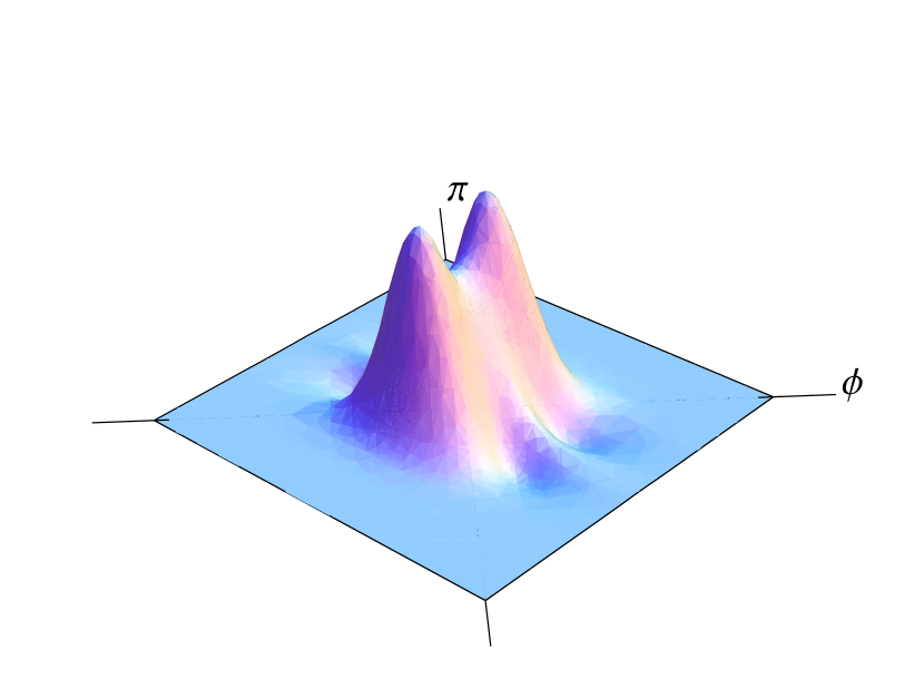
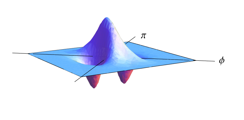
Figure 5: Wigner transform of the density matrix described by equations (61) and (62), with $\eta_{0}\neq 0$ only. We used $\eta_{0}>0$ (left) and $\eta_{0}<0$ (right). The peak structure of our state in phase space, that was so simple for Gaussian density matrices, is much more complicated. Some regions in phase space have a negative value of the Wigner function, indicating a breakdown of the use of a Wigner function as a convenient measure of probability.

To gain some intuitive understanding of what our density matrix looks like, let us consider figure 5. Here, we show the Wigner transform of equation (61) using (62), with $\eta_{1}=0=\eta_{2}$. Clearly, the quartic corrections change the peak structure of our state in phase space. Moreover, some regions in phase space now have a negative Wigner function. This nicely illustrates the limitations of using the Wigner function as a probability density on our phase space as soon as non-Gaussianities (due to interactions) are included, i.e.: equation (23) holds only approximately in this case.

In order to calculate the entropy, we need ${\rm Tr}[\hat{\rho}_{4}^{1+\epsilon}]$ as before (cf. equation (36)). To linear order in $\delta\rho_{\rm ng}$ we have:

$${\rm Tr}[\hat{\rho}_{4}^{1+\epsilon}]=\left(\frac{{\cal N}_{4}}{{\cal N}_{\rm g}}\right)^{1+\epsilon}\Big{(}{\rm Tr}[\hat{\rho}_{\rm g}^{1+\epsilon}]+(1+\epsilon){\rm Tr}[\hat{\rho}_{\rm g}^{1+\epsilon}\delta\hat{\rho}_{\rm ng}]\Big{)}\,.$$ (64)

The first term in the parentheses is just the Gaussian result (36) while the latter term can be evaluated by making use of the formulae in Appendix A. Expanding to linear order in $\epsilon$, the equation above yields:

$${\rm Tr}[\hat{\rho}_{4}^{1+\epsilon}] = 1+\epsilon\Big{[}\ln(1-\alpha)+\frac{\alpha}{1-\alpha}\ln(\alpha)\Big{]}+\epsilon\bigg{[}\frac{3}{4}\frac{\eta_{0}+\eta_{0}^{*}}{[2(a_{\mathrm{R}}-c)]^{2}}\Big{(}\frac{4\alpha}{1-\alpha^{2}}\ln(\alpha)-1\Big{)}$$ (65)

$$\hskip 28.45274pt+\,\frac{3}{4}\frac{\eta_{1}+\eta_{1}^{*}}{[2(a_{\mathrm{R}}-c)]^{2}}\Big{(}\frac{1+\alpha}{1-\alpha}\ln(\alpha)-1\Big{)}+\frac{3}{4}\frac{\eta_{2}}{[2(a_{\mathrm{R}}-c)]^{2}}\Big{(}\frac{4}{3}\frac{1+\alpha+\alpha^{2}}{1-\alpha^{2}}\ln(\alpha)-1\Big{)}\bigg{]}\,.\qquad$$

As expected, we see that the entropy naturally splits into a Gaussian and a non-Gaussian contribution:

$$S_{4}(t)=S_{\rm g}(t)+\delta S_{4}(t)\,,$$ (66a)

where $$S_{\rm g}$$ is the Gaussian entropy as before, and where:

$$\delta S_{4}(t) = \frac{\eta_{0}+\eta_{0}^{*}}{[2(a_{\mathrm{R}}\!-\!c)]^{2}}\left(\frac{3n(1+n)}{1+2n}\ln\left(\frac{1+n}{n}\right)+\frac{3}{4}\right)+\frac{3}{4}\frac{\eta_{1}+\eta_{1}^{*}}{[2(a_{\mathrm{R}}\!-\!c)]^{2}}\left((1+2n)\ln\left(\frac{1+n}{n}\right)+1\right)$$ (66b)

$$+\,\frac{\eta_{2}}{[2(a_{\mathrm{R}}\!-\!c)]^{2}}\left(\frac{1+3n+3n^{2}}{1+2n}\ln\left(\frac{1+n}{n}\right)+\frac{3}{4}\right)\,.$$

This is the main result of this section and intuitive in the following sense: just as in the first non-Gaussian example above, we see that positive kurtosis parameters $\{\eta_{0R},\eta_{1R},\eta_{2}\}>0$, tend to make the effective state’s width $(a_{\mathrm{R}}-c)^{-1/2}$ larger, which increases the area in phase space the state occupies, which in turn increases the entropy. If however $\{\eta_{0R},\eta_{1R},\eta_{2}\}<0$, the phase space area shrinks, which in turn decreases the entropy. The statements above hold for any statistical particle number $0\ll n<\infty$, with the exception of $n\rightarrow 0$, where, just as in the case studied above, a weak logarithmic divergence occurs when $\eta_{1R}\neq 0$ or $\eta_{2}\neq 0$. Notice finally that $\Im[\eta_{0}]$ and $\Im[\eta_{1}]$ again do not participate in entropy generation, but rather contribute to the squeezing of the state.

Kurtosis and skewness in quantum mechanics, studied in this section, occur also in interacting quantum field theories which we discuss next.

V Entropy in Scalar Field Theory

The quantum mechanical expressions for the Gaussian and non-Gaussian entropies that we have developed for pedagogical reasons in sections II, III and IV for a single particle density matrix can be generalised to field theory. We firstly need to consider correlators in quantum field theory however.

V.1 Equal Time Correlators in Scalar Field Theory

Let us now proceed analogous to equation (10) and write the density matrix operator for our system in the field amplitude basis in Schrödinger’s picture (see e.g. Koksma:2007uq ):

$$\hat{\rho}_{\mathrm{g}}=\int{\cal D}\phi\int{\cal D}\phi^{\prime}|\phi\rangle\rho_{\mathrm{g}}[\phi,\phi^{\prime};t]\langle\phi^{\prime}|\,,$$ (67)

where:

$$\rho_{\mathrm{g}}[\phi,\phi^{\prime};t]={\cal N}\exp\left(-\phi^{T}\!\cdot A\cdot\phi-{\phi^{\prime}}^{T}\!\cdot B\!\cdot\!\phi^{\prime}+2\phi^{T}\!\cdot C\!\cdot\!\phi^{\prime}\right)\,,$$ (68)

where ${\cal D}\phi=\prod_{\vec{x}\in V}\mathrm{d}\phi(\vec{x}\,)$ and $|\phi\rangle=\prod_{\vec{x}\in V}|\phi(\vec{x}\,)\rangle$. A few words on the notation first. We shall consider $\phi=\phi(\vec{x})$ as a vector whose components are labelled by $\vec{x}$. Moreover, $A(\vec{x},\vec{y},t)$ can be viewed as a matrix, such that $A\cdot\phi$ is a vector again, where a $\cdot$ denotes matrix multiplication which, for the case at hand, is nothing but an integral over $D-1$ dimensional space. Hence, quantities like $\phi^{\mathrm{T}}\cdot A\cdot\phi$ are scalars and involve two integrals over space. Note that at this point we do not assume that $A$ is homogeneous, i.e.: $A(\vec{x},\vec{y},t)\neq A(\vec{x}-\vec{y},t)$, but rather keep any possible off-diagonal terms for generality.

Our density matrix (68) is hermitian, such that we have $A^{*}(\vec{x},\vec{y},t)=B(\vec{x},\vec{y},t)$ and $C^{*}(\vec{x},\vec{y},t)=C(\vec{x},\vec{y};t)$, where we also used $A(\vec{x},\vec{y},t)=A(\vec{y},\vec{x},t)$ and $C(\vec{x},\vec{y},t)=C(\vec{y},\vec{x};t)$. The normalisation ${\cal N}$ of $\rho[\phi,\phi^{\prime};t]$ can be determined from the standard requirement ${\rm Tr}[\hat{\rho}]=1$:

$${\cal N}=\left({\rm det}\left[\frac{2(A_{\mathrm{R}}-C)}{\pi}\,\right]\right)^{1/2}\,,$$ (69)

where we note that the hermitian part $A_{\mathrm{h}}$ of $A$ is real and symmetric such that $A_{\mathrm{h}}=A_{\mathrm{R}}$.

Just as in the quantum mechanical case, we need to calculate the three non-trivial Gaussian correlators which completely characterise the properties of our Gaussian state. In order to calculate these correlators, we need to have an expression for the statistical propagator as in equation (3) which, given some initial density matrix $\hat{\rho}(t_{0})$, is in the Heisenberg picture defined by:

$$F(\vec{x},t;\vec{y},t^{\prime})={\rm Tr}\left[\hat{\rho}(t_{0})\hat{\phi}(\vec{x},t)\hat{\phi}(\vec{y},t^{\prime})\right]\,.$$ (70)

Let us begin by calculating:

$$\langle\hat{\phi}(\vec{x})\hat{\phi}(\vec{y})\rangle=F(\vec{x},\vec{y};t)={\rm Tr}\left[\hat{\rho}(t)\hat{\phi}(\vec{x}\,)\hat{\phi}(\vec{y}\,)\right]\,,$$ (71)

where we have made use of the Heisenberg evolution equation for operators. It is convenient to add a source current $j(\vec{x},t)$ to the density matrix (67), such that $\rho$ becomes:

$$\rho_{\mathrm{g}}^{j}[\phi,\phi^{\prime};t]={\cal N}\exp\left(-\phi^{T}\!\cdot A\cdot\phi-{\phi^{\prime}}^{T}\!\cdot A^{{\dagger}}\!\cdot\!\phi^{\prime}+2\phi^{T}\!\cdot C\!\cdot\!\phi^{\prime}+j^{T}\!\cdot\phi+{j^{\prime}}^{T}\!\cdot\phi^{\prime}\right)\,,$$ (72)

in terms of which equation (71) can be rewritten as:

$$F(\vec{x},\vec{y};t) = \frac{\delta}{\delta j(\vec{x}\,)}\frac{\delta}{\delta j(\vec{y}\,)}\int{\cal D}\phi\rho^{j}_{\mathrm{g}}[\phi,\phi;t]\Big{|}_{j=j^{\prime}=0}$$ (73a)

$$= \frac{\delta}{\delta j(\vec{x}\,)}\frac{\delta}{\delta j(\vec{y}\,)}\int{\cal D}\tilde{\phi}\,{\cal N}\left.\exp\left(-2\tilde{\phi}^{T}\!\cdot(A_{\mathrm{R}}-C)\cdot\tilde{\phi}\right)\exp\left(\frac{1}{8}(j+j^{\prime})^{T}\!\cdot(A_{\mathrm{R}}-C)^{-1}\cdot(j+j^{\prime})\right)\right|_{j=j^{\prime}=0}$$

$$= \frac{1}{4}(A_{\mathrm{R}}-C)^{-1}(\vec{x},\vec{y};t)\,.$$

We also need the other correlators:

$$\frac{1}{2}\langle\{\hat{\phi}(\vec{x}),\hat{\pi}(\vec{y})\}\rangle = \partial_{t^{\prime}}F(\vec{x},t;\vec{y},t^{\prime})|_{t=t^{\prime}}=\frac{1}{2}{\rm Tr}[\hat{\rho}_{\mathrm{g}}(t)\{\hat{\phi}(\vec{x}\,),\hat{\pi}(\vec{y}\,)\}]=-\frac{\hbar}{2}(A_{\mathrm{R}}-C)^{-1}\cdot A_{\mathrm{I}}(\vec{x},\vec{y};t)$$ (73b)

$$\frac{1}{2}\langle\{\hat{\pi}(\vec{x}),\hat{\pi}(\vec{y})\}\rangle = \partial_{t}\partial_{t^{\prime}}F(\vec{x},t;\vec{y},t^{\prime})|_{t=t^{\prime}}=\frac{1}{2}{\rm Tr}[\hat{\rho}_{\mathrm{g}}(t)\{\hat{\pi}(\vec{x}\,),\hat{\pi}(\vec{y}\,)\}]$$

$$= \hbar^{2}\!\left[\frac{1}{2}A^{{\dagger}}\!\cdot\!(A_{\mathrm{R}}\!-C)^{-1}\!\cdot\!A\!+\!A\cdot\!(A_{\mathrm{R}}\!-C)^{-1}\!\cdot A^{{\dagger}}\!-C\!\cdot\!(A_{\mathrm{R}}\!-C)^{-1}\!\cdot C\!\right](\vec{x},\vec{y};t)\,.$$

We have moreover made use of $\langle\phi^{\prime}|\hat{\pi}|\phi\rangle=-\imath\hbar\frac{\delta}{\delta\phi^{\prime}}\delta[\phi^{\prime}-\phi]$. As a check one can verify that:

$${\rm Tr}(\hat{\rho}_{\mathrm{g}}(t)[\hat{\phi}(\vec{x}\,),\hat{\pi}(\vec{y}\,)])=\imath\hbar\delta^{\scriptscriptstyle{D}-1}(\vec{x}-\vec{y}\,)\,.$$ (74)

Combining the equations above we find:

$$\Delta^{2}(\vec{x},\vec{y};t) = \frac{4}{\hbar^{2}}\left[\left\langle\hat{\phi}\hat{\phi}\right\rangle\cdot\left\langle\hat{\pi}\hat{\pi}\right\rangle-\frac{1}{4}\left\langle\{\hat{\phi},\hat{\pi}\}\right\rangle\cdot\left\langle\{\hat{\phi},\hat{\pi}\}\right\rangle\right](\vec{x},\vec{y};t)$$ (75)

$$= (A_{\mathrm{R}}-C)^{-1}\cdot(A_{\mathrm{R}}+C)(\vec{x},\vec{y};t)\,.$$

This is the desired field theoretic generalisation of the Gaussian invariant $\Delta^{2}$ in equation (29). Notice that the result above applies for general non-diagonal Gaussian density matrices. This is an important quantity because, just as in the quantum mechanical case, $\Delta$ will be the conserved quantity under any quadratic Hamiltonian evolution. Since the von Neumann entropy is also conserved in this case, it is natural to expect that $S_{\mathrm{vN}}=S_{\mathrm{vN}}[\Delta]$.

Of course, if we are interested in problems in which the hamiltonian density is only time dependent, one can make use of spatial translation invariance of the correlators, such that the equal time statistical correlator is homogeneous: $F(\vec{x},\vec{y};t)\rightarrow\tilde{F}(\vec{x}-\vec{y},t)$. In this case it is beneficial to Fourier transform according to:

$$\tilde{F}(\vec{k},t)=\int\mathrm{d}^{\scriptscriptstyle{D}-1}(\vec{x}-\vec{y})\tilde{F}(\vec{x}-\vec{y},t)\mathrm{e}^{-\imath\vec{k}\cdot(\vec{x}-\vec{y})}\,,$$ (76)

such that equation (75) becomes local in momentum space and reduces to the result known in the literature:

$$\tilde{\Delta}^{2}(\vec{k};t) = \frac{4}{\hbar^{2}}\left.\left[\tilde{F}(\vec{k},t,t)\partial_{t}\partial_{t^{\prime}}\tilde{F}(\vec{k},t,t^{\prime})-\left(\partial_{t^{\prime}}\tilde{F}(\vec{k},t,t^{\prime})\right)^{2}\right]\right|_{t=t^{\prime}}$$ (77)

$$= \frac{(\tilde{A}_{\mathrm{R}}+\tilde{C})(\vec{k},t)}{(\tilde{A}_{\mathrm{R}}-\tilde{C})(\vec{k},t)}\,.$$

This representation is particularly useful in problems with spatial translational symmetry, such as cosmology Brandenberger:1992jh ; Campo:2008ij .

V.2 Entropy of a Gaussian state in Scalar Field Theory

Let us now discuss the von Neumann entropy (1) of the Gaussian density matrix (67) by using the replica method (35). One can proceed analogous to section III. Some subtleties arise however as we deal with a system with infinite degrees of freedom. For this reason, we nevertheless include an outline of the proof in appendix B. The entropy for a quantum system that can be described by a Gaussian density matrix is given by:

$$S_{\rm vN}={\rm Tr}\left[\frac{\Delta+\mathbb{I}}{2}\cdot\ln\left(\frac{\Delta+\mathbb{I}}{2}\right)-\frac{\Delta-\mathbb{I}}{2}\cdot\ln\left(\frac{\Delta-\mathbb{I}}{2}\right)\right]\,.$$ (78)

We denote the identity matrix by $\mathbb{I}=\delta^{\scriptscriptstyle{D}-1}(\vec{x}-\vec{y})$. As in the quantum mechanical case, we can define the generalised statistical particle number density correlator $n=n(\vec{x},\vec{y},t)$ as:

$$n=\frac{\Delta-\mathbb{I}}{2}\,,$$ (79)

in terms of which the entropy (78) reads:

$$S_{\rm vN}={\rm Tr}\left[(n+\mathbb{I})\cdot\ln\left(n+\mathbb{I}\right)-n\cdot\ln\left(n\right)\right]\,.$$ (80)

In the limit when $\|n\|\gg 1$, in the sense that for the diagonalised matrix its diagonal entries of interest are large, we can expand the logarithms in (80) to get for the entropy, $S_{\rm vN}\approx{\rm Tr}[\ln(n)+\mathbb{I}+{\cal O}(n^{-1})]$, which nearly coincides with the Wigner entropy $S_{\cal W}$ in field theory, cf. equation (32). Equations (80) and (78) represent the von Neumann entropy of a general Gaussian state in scalar field theory and are the main result of this section.

In the homogeneous limit, we can again Fourier transform and equation (78) reduces to:

$$S_{\rm vN}=V\int\frac{\mathrm{d}^{3}\mathbf{k}}{(2\pi)^{3}}\left[\frac{\Delta(\mathbf{k},t)+1}{2}\ln\left(\frac{\Delta(\mathbf{k},t)+1}{2}\right)-\frac{\Delta(\mathbf{k},t)-1}{2}\ln\left(\frac{\Delta(\mathbf{k},t)-1}{2}\right)\right]\,,$$ (81)

where the volume factor arises because of the trace. The limit $\Delta(\mathbf{k},t)\gg 1$ basically agrees with Brandenberger:1992jh .

V.3 Entropy of a Non-Gaussian state in Scalar Field Theory

Analogous to the one particle non-Gaussian entropy discussed in section IV, let us generalise that result to the field theoretical case. The non-Gaussian density matrix $\hat{\rho}_{2}$ in equation (67) generalises to:

$$\hat{\rho}_{2}=\int{\cal D}\phi\int{\cal D}\phi^{\prime}|\phi\rangle\rho_{2}[\phi,\phi^{\prime};t]\langle\phi^{\prime}|\,,$$ (82a)

where:

$$\rho_{2}[\phi,\phi^{\prime};t] = {\cal N}_{2}\left[1+\zeta_{0}\cdot\phi+\zeta_{0}^{\dagger}\cdot\phi^{\prime}+\phi^{T}\cdot\zeta_{1}\cdot\phi+{\phi^{\prime}}^{T}\cdot\zeta_{1}^{\dagger}\cdot\phi^{\prime}+\phi^{T}\cdot\zeta_{2}\cdot{\phi^{\prime}}+{\phi^{\prime}}^{T}\cdot\zeta_{2}^{\dagger}\cdot\phi\right]\rho_{0}[\phi,\phi^{\prime};t]$$ (82b)

$$\rho_{0}[\phi,\phi^{\prime};t] = \exp\left[-\phi^{T}\!\cdot A\cdot\phi-{\phi^{\prime}}^{T}\!\cdot A^{{\dagger}}\!\cdot\!\phi^{\prime}+\phi^{T}\!\cdot C\!\cdot\!\phi^{\prime}+{\phi^{\prime}}^{T}\!\cdot C^{T}\cdot\!\phi\right]\,,$$ (82c)

We could of course perform a similar shift in the exponent as we have done before in equation (54) in which case the resulting equation for the entropy would formally be exact, i.e: we do not assume yet that the non-Gaussian contributions are small. If we want to expand around the Gaussian result however, we can only perform the integral if we assume that all correlators, including the non-Gaussian ones, are homogeneous, i.e.: they are only a function of the difference of their coordinates $A(\vec{x},\vec{y},t)=A(\vec{x}-\vec{y},t)$. The Fourier transform of equation (82) is:

$$\rho_{2}[\phi,\phi^{\prime};t]=\prod_{\mathbf{k}}{\cal N}_{2,\mathbf{k}}\exp\left[-\bar{A}(\mathbf{k},t)|\phi(\mathbf{k})|^{2}-\bar{A}^{\ast}(\mathbf{k},t)|\phi^{\prime}(\mathbf{k})|^{2}+2\bar{C}(\mathbf{k},t)\phi^{\ast}(\mathbf{k})\phi^{\prime}(\mathbf{k})\right]+{\cal O}(\zeta_{i}^{2})\,,$$ (83)

where we have set $\zeta_{0}=0$ as before, as it will not induce an entropy shift. Also, the product over the momenta is only over half of the Fourier space. Moreover, we have absorbed the small non-Gaussian contributions in the functions $\bar{A}$ and $\bar{C}$ as in the quantum mechanical case:

$$A(\mathbf{k},t) \rightarrow \bar{A}(\mathbf{k},t)=A(\mathbf{k},t)-\zeta_{1}(\mathbf{k},t)$$ (84a)

$$C(\mathbf{k},t) \rightarrow \bar{C}(\mathbf{k},t)=C(\mathbf{k},t)+\zeta_{2}(\mathbf{k},t)\,,$$ (84b)

Now we can read off the result for the entropy in Fourier space in equation (81) as:

$$S_{\rm vN}=V\int\frac{\mathrm{d}^{3}\mathbf{k}}{(2\pi)^{3}}\left[\frac{\bar{\Delta}(\mathbf{k},t)+1}{2}\ln\left(\frac{\bar{\Delta}(\mathbf{k},t)+1}{2}\right)-\frac{\bar{\Delta}(\mathbf{k},t)-1}{2}\ln\left(\frac{\bar{\Delta}(\mathbf{k},t)-1}{2}\right)\right]\,,$$ (85)

Assuming that $\zeta_{i}(\mathbf{k},t)\ll 1$ we can derive the change in entropy to linear order in $\zeta_{i}$. The result is:

$$S_{2}(t)=S_{\mathrm{g}}(t)+\delta S_{2}(t)\,,$$ (86a)

where $$S_{\mathrm{g}} \delta S_{2}$$ is the Gaussian contribution and is an entropy shift given by:

$$\delta S_{2} = V\int\frac{\mathrm{d}^{3}\mathbf{k}}{(2\pi)^{3}}\Bigg{[}\left(\frac{\zeta_{1R}(\mathbf{k},t)}{A_{\mathrm{R}}(\mathbf{k},t)-C(\mathbf{k},t)}+\frac{1+2n(\mathbf{k},t)+2n^{2}(\mathbf{k},t)}{2n(\mathbf{k},t)(1+n(\mathbf{k},t))}\frac{\zeta_{2}(\mathbf{k},t)}{A_{\mathrm{R}}(\mathbf{k},t)-C(\mathbf{k},t)}\right)$$ (86b)

$$\qquad\qquad\qquad\times\frac{n(\mathbf{k},t)(1+n(\mathbf{k},t))}{1+2n(\mathbf{k},t)}\ln\left(\frac{1+n(\mathbf{k},t)}{n(\mathbf{k},t)}\right)\Bigg{]}\,,$$

where, of course, $n(\mathbf{k},t)=(\Delta(\mathbf{k},t)-1)/2$. This result is the field theoretic generalisation of the quantum mechanical entropy (58). It can be applied to mildly non-Gaussian states in field theory, which, apart from being mixed, also contain small one particle contributions.

The field theoretical generalisation of the second example presented in section IV.2 is hard to solve for, even in the homogeneous case, as it is non-local in Fourier space.

V.4 Example: A Scalar Field with a Changing Mass

As a simple illustration of the ideas presented above, let us investigate the effect of a changing mass on the Gaussian entropy for a scalar field. This is maybe not a very exciting example, as no entropy is generated of course in free theories, it nevertheless provides an intuitive way of how the Wigner function can be used. Let us consider the action of a free scalar field:

$$S[\phi]=\int\mathrm{d}^{4}\!x\left\{-\frac{1}{2}\partial_{\mu}\phi(x)\partial_{\nu}\phi(x)\eta^{\mu\nu}-\frac{1}{2}m^{2}_{\phi}(t)\phi^{2}(x)\right\}\,,$$ (87)

where as usual $\eta_{\mu\nu}={\rm diag}(-1,1,1,1)$ is the Minkowski metric, and where we consider the following behaviour of the mass $m_{\phi}(t)$ of the scalar field, mediated for example by some other Higgs-like scalar field:

$$m^{2}_{\phi}(t)=\left(A+B\tanh(\rho t)\right)\,.$$ (88)

The equation of motion following from (87) reads:

$$\left(\partial_{t}^{2}-\partial_{i}^{2}+m^{2}_{\phi}(t)\right)\phi(x)=0\,,$$ (89)

Let us quantise our fields in $D$-dimensions by making use of creation and annihilation operators:

$$\hat{\phi}(x)=\int\frac{\mathrm{d}^{\scriptscriptstyle{D}-1}\vec{k}}{(2\pi)^{\scriptscriptstyle{D}-1}}\left(\hat{a}_{\vec{k}}\,\phi_{k}(t)e^{i\vec{k}\cdot\vec{x}}+\hat{a}_{\vec{k}}^{{\dagger}}\,\phi_{k}^{\ast}(t)e^{-i\vec{k}\cdot\vec{x}}\right)\,.$$ (90)

The annihilation operator acts on the vacuum as usual $\hat{a}_{\vec{k}}|0\rangle=0$. We impose the following commutation relations: $[\hat{a}_{\vec{k}},\hat{a}_{\vec{k^{\prime}}}^{{\dagger}}]=(2\pi)^{\scriptscriptstyle{D}-1}\delta^{\scriptscriptstyle{D}-1}(\vec{k}-\vec{k^{\prime}})$. The mode functions $\phi_{k}(t)$ of $\phi(x)$, defined by relation (90) thus obey:

$$\left(\partial_{t}^{2}+\omega^{2}(t)\right)\phi_{k}(t)=0\,,$$ (91)

where $k=\|\vec{k}\|$ and $\omega^{2}(t)=k^{2}+m^{2}_{\phi}(t)$. Using equation (71) with $\hat{\rho}(t_{0})=|0\rangle\langle 0|$, we see that the mode functions determine the statistical propagator completely:

$$F_{\phi}(k,t,t^{\prime})=\frac{1}{2}\left\{\phi_{k}(t^{\prime})\phi_{k}^{\ast}(t)+\phi_{k}(t)\phi_{k}^{\ast}(t^{\prime})\right\}\,.$$ (92)

The solution of (91) which behaves as a positive frequency mode in the asymptotic past, i.e.: $\lim_{t\rightarrow-\infty}\phi_{k}^{\mathrm{in}}(t)=\exp\left[-\imath\omega_{\mathrm{in}}t\right]/\sqrt{2\omega_{\mathrm{in}}}$, can be expressed in terms of Gauss’ hypergeometric function ${}_{2}F_{1}$ (see Bernard:1977pq ; Birrell:1982ix ):

$$\phi_{k}^{\mathrm{in}}(t)=\frac{1}{\sqrt{2\omega_{\mathrm{in}}}}\exp\left[-\imath\omega_{+}t-\imath\frac{\omega_{-}}{\rho}\log\{2\cosh(\rho t)\}\right]\phantom{1}_{2}F_{1}\left(1+\imath\frac{\omega_{-}}{\rho},\imath\frac{\omega_{-}}{\rho};1-\imath\frac{\omega_{\mathrm{in}}}{\rho};\frac{1}{2}\{1+\tanh(\rho t)\}\right)\,,$$ (93)

where we defined $\omega_{\mathrm{in}}=(k^{2}+A-B)^{\frac{1}{2}}$, $\omega_{\mathrm{out}}=(k^{2}+A+B)^{\frac{1}{2}}$ and $\omega_{\pm}=(\omega_{\mathrm{out}}\pm\omega_{\mathrm{in}})/2$. Having the mode functions at our disposal, we can find the rather cumbersome expressions for the exact statistical propagator. The statistical propagator in turn fixes the phase space area through equation (77), yielding $\Delta_{k}(t)=1$ such that:

$$S_{k}(t)=0\,.$$ (94)

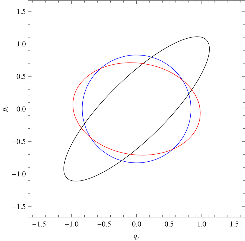
Figure 6: Squeezing of the Gaussian phase space in the Wigner representation due to a changing mass. We used $k/\rho=0.2$ and $m/\rho$ changes from 0 to 4 where the mass changes most rapidly at $t\rho=5$. For early times $t\rho=0$, the Gaussian phase space is a perfect circle (blue). Already for $t\rho=2$ a little squeezing is visible (red) and at late times $t\rho=9$ this is manifest (black). The coordinates $p_{r}$ and $q_{r}$ have been rescaled for dimensional reasons: $p_{r}=p\sqrt{\omega(t)}$ and $q_{r}=q/\sqrt{\omega(t)}$.

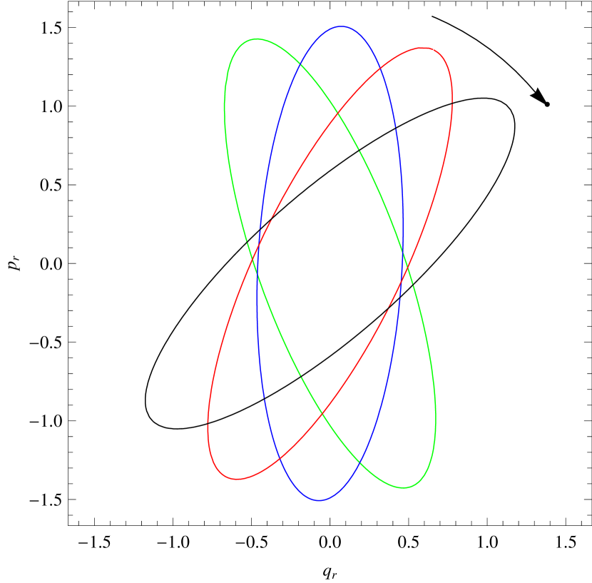
Figure 7: Rotation of the Gaussian phase space in the Wigner representation due to a mass that has changed. We used the same parameters as in figure 7. The squeezed phase space ellipses are plotted at times $t\rho=9.5$ (green), $t\rho=9.6$ (blue), $t\rho=9.7$ (red) and $t\rho=9.8$ (black). The rotation is clearly visible and its direction is indicated by the arrow. This can be understood from realising that an arbitrary squeezed state can be interpreted as a superposition of ordinary coherent states and the knowledge that the latter show the same rotating behaviour.

We thus conclude that a changing mass does not change the entropy for a free scalar field. Let us now examine the same process in Wigner space. Of course, we will reach a similar conclusion (94) but Wigner space is much more suited to visualise the process neatly. The statistical propagator is also the essential building block for the Wigner function which can be appreciated from generalising equations (28) and (18) to:

$$\alpha_{\mathrm{w}}(k,t) = \frac{1}{2F_{\phi}(k,t,t)}$$ (95a)

$$\beta_{\mathrm{w}}(k,t) = \frac{2F_{\phi}(k,t,t)}{\Delta_{k}^{2}(t)}$$ (95b)

$$p_{\mathrm{c}} = -\frac{\partial_{t}F_{\phi}(k,t,t^{\prime})|_{t=t^{\prime}}}{F_{\phi}(k,t,t)}$$ (95c)

$$\mathcal{M}_{k}(t) = \frac{2}{\Delta_{k}(t)}\,.$$ (95d)

We can thus plot cross-sections of the 2-dimensional Gaussian phase space distribution in the Wigner representation. In figure 7 we depict the squeezing of the Gaussian phase space due to the changing mass. At early times, the state is still in an unsqueezed vacuum. At $t\rho=2$ some squeezing is visible, whereas at late times $t\rho=9$ this is manifest. Despite the effect of the changing mass on the accessible phase space in Wigner space, the area of the ellipse remains constant throughout the whole process as expected from equation (94). At late times, when the mass has settled to its final constant value $m/\rho=4$, the squeezed ellipse rotates in Wigner space, which we depict in figure 7, but it is not squeezed any further. The rotation can be anticipated by the intuitive notion that an arbitrary squeezed state can be thought of as a superposition of coherent states (just imagine that the ellipse is replaced by a number of circles displaced from the origin). Coherent states that are displaced from the origin rotate in time.

VI Conclusion

We have formally developed a novel approach to decoherence in quantum field theory: neglecting observationally inaccessible correlators will give rise to an increase in the entropy of the system. This is inspired by realising that correlators are measured in quantum field theories and that higher order n-point functions are usually perturbatively suppressed. An important advantage of this approach is that the procedure of renormalisation can systematically be implemented in this framework.

We have shown how knowledge about the correlators of a system affects the notion of the entropy associated to that state in two cases: we firstly calculated the entropy of a general Gaussian state. This entropy can be expressed purely in terms of the three equal time correlators characterising the Gaussian state. Moreover, all three correlators can be obtained from the statistical propagator which opens the possibility to study quantum corrections on the entropy in an interacting quantum field theory in a systematic manner. Secondly, we calculated the entropy for two specific types of non-Gaussian states. Firstly, we assumed that the state of the system can be described by an admixture of the ground state and a small contribution of the first excited state. This yields a small correction to the Gaussian entropy. Secondly, in the quantum mechanical case, we calculated an expression for the entropy in case our observer could probe a specific type of kurtosis of the ground state. This also changes the entropy that the observes associates to the state.

We also outlined the use and limitations of the Wigner function, the Wigner transform of the density matrix of a system. In particular, we have shown that $\Delta$, the fundamental quantity constructed from various correlators that fixes the entropy, indeed coincides with the phase space area in Wigner space.

This is a rather phenomenological discussion, connecting the notion of entropy, correlators and phase space area in quantum field theory. Although we have outlined various mechanisms how entropy could be generated, we have in the present paper not applied our ideas to concrete systems. We refer the reader to e.g. Giraud:2009tn ; Koksma:2009wa ; Koksma:2010 for specific examples of how entropy is generated in interacting quantum field theories in an out-of-equilibrium setting.

Acknowledgements

JFK and TP thank Theo Ruijgrok and gratefully acknowledge the financial support from FOM grant 07PR2522 and by Utrecht University. The authors also gratefully acknowledge the hospitality of the Nordic Institute for Theoretical Physics (NORDITA) during their stay at the “Electroweak Phase Transition” workshop in June, 2009.

Appendix A Useful Integrals

Here we quote some integrals that are used in section IV. The three integrals are:

$$I_{\eta 0}(\epsilon) = \int_{-\infty}^{\infty}\mathrm{d}x_{0}\cdots\int_{-\infty}^{\infty}\mathrm{d}x_{\epsilon}\left(\eta_{0}x_{\epsilon}^{4}+\eta_{0}^{*}x_{0}^{4}\right)\exp\left[-2a_{\mathrm{R}}(x_{0}^{2}+\cdots+x_{\epsilon}^{2})+2c(x_{0}x_{1}+\cdots+x_{\epsilon}x_{0})\right]$$ (96)

$$\hskip 142.26378pt=\,(\eta_{0}+\eta_{0}^{*})\frac{3}{4}\frac{\pi^{\frac{1+\epsilon}{2}}}{(2\beta)^{\frac{5+\epsilon}{2}}}\frac{(1-\alpha^{2+2\epsilon})^{2}}{(1-\alpha^{2})^{2}(1-\alpha^{1+\epsilon})^{5}}$$

$$I_{\eta 1}(\epsilon) = \int_{-\infty}^{\infty}\mathrm{d}x_{0}\cdots\int_{-\infty}^{\infty}\mathrm{d}x_{\epsilon}\left(\eta_{1}x_{\epsilon}^{3}x_{0}+\eta_{1}^{*}x_{\epsilon}x_{0}^{3}\right)\exp\left[-2a_{\mathrm{R}}(x_{0}^{2}+\cdots+x_{\epsilon}^{2})+2c(x_{0}x_{1}+\cdots+x_{\epsilon}x_{0})\right]$$ (97)

$$\hskip 142.26378pt=\,(\eta_{1}+\eta_{1}^{*})\frac{3}{4}\frac{\pi^{\frac{1+\epsilon}{2}}}{(2\beta)^{\frac{5+\epsilon}{2}}}\frac{\alpha(1+\alpha^{-1+\epsilon})(1-\alpha^{2+2\epsilon})}{(1-\alpha^{2})^{2}(1-\alpha^{1+\epsilon})^{4}}$$

$$I_{\eta 2}(\epsilon) = \int_{-\infty}^{\infty}\mathrm{d}x_{0}\cdots\int_{-\infty}^{\infty}\mathrm{d}x_{\epsilon}\left(\eta_{2}x_{\epsilon}^{2}x_{0}^{2}\right)\exp\left[-2a_{\mathrm{R}}(x_{0}^{2}+\cdots+x_{\epsilon}^{2})+2c(x_{0}x_{1}+\cdots+x_{\epsilon}x_{0})\right]$$ (98)

$$\hskip 142.26378pt=\,\eta_{2}\frac{1}{4}\frac{\pi^{\frac{1+\epsilon}{2}}}{(2\beta)^{\frac{5+\epsilon}{2}}}\frac{(1+\alpha^{2})^{2}(1+\alpha^{-2+2\epsilon})-\alpha^{4}(1+\alpha^{-6+2\epsilon})+6\alpha^{1+\epsilon}}{(1-\alpha^{2})^{2}(1-\alpha^{1+\epsilon})^{3}}\,,\qquad$$

where $\epsilon\geq 0$ is an integer. The first non-trivial check of these integrals is to set $\epsilon=0$, in which case their sum gives the (inverse) normalisation constant (63),

$$I_{\eta 0}(0)+I_{\eta 1}(0)+I_{\eta 2}(0)=\sqrt{\frac{\pi}{2(a_{\mathrm{R}}-c)}}\frac{3}{4}\frac{\eta_{0}+\eta_{0}^{*}+\eta_{1}+\eta_{1}^{*}+\eta_{2}}{[2(a_{\mathrm{R}}-c)]^{2}}={\cal N}_{4}^{-1}-{\cal N}_{\rm g}^{-1}\,.$$

Moreover, we encourage the reader to check the integrals for some other values of $\epsilon$. By performing direct integrations we have checked the integrals (96–98) for $\epsilon=1,2,3,4,5$, and they all give the correct answer. Since the expressions (96–98) are analytic in $\epsilon$ when $0<\alpha<1$, they can be uniquely analytically extended to complex $\epsilon$’s in that range of $\alpha$, based on which we calculate the von Neumann entropy in section IV. For the entropy calculation we need to expand the integrals (96–98) around $\epsilon=0$ up to linear order in $\epsilon$. From equation (64) we see that it is convenient to multiply the integrals with ${\cal N}_{\rm g}^{1+\epsilon}=[2(a_{\mathrm{R}}-c)/\pi]^{(1+\epsilon)/2}$,

$${\cal N}_{\rm g}^{1+\epsilon}I_{\eta 0}(\epsilon) = \frac{3}{4}\frac{\eta_{0}+\eta_{0}^{*}}{[2(a_{\mathrm{R}}-c)]^{2}}\bigg{\{}1+\epsilon\bigg{[}\ln(1-\alpha)+\frac{\alpha(5+\alpha)}{1-\alpha^{2}}\ln(\alpha)\bigg{]}\bigg{\}}$$ (99)

$${\cal N}_{\rm g}^{1+\epsilon}I_{\eta 1}(\epsilon) = \frac{3}{4}\frac{\eta_{1}+\eta_{1}^{*}}{[2(a_{\mathrm{R}}-c)]^{2}}\bigg{\{}1+\epsilon\bigg{[}\ln(1-\alpha)+\frac{1+3\alpha+2\alpha^{2}}{1-\alpha^{2}}\ln(\alpha)\bigg{]}\bigg{\}}$$ (100)

$${\cal N}_{\rm g}^{1+\epsilon}I_{\eta 2}(\epsilon) = \frac{3}{4}\frac{\eta_{2}}{[2(a_{\mathrm{R}}-c)]^{2}}\bigg{\{}1+\epsilon\bigg{[}\ln(1-\alpha)+\frac{1}{3}\frac{4+7\alpha+7\alpha^{2}}{1-\alpha^{2}}\ln(\alpha)\bigg{]}\bigg{\}}\,,\qquad$$ (101)

where we used $a_{\mathrm{R}}/c=(1+\alpha^{2})/(2\alpha)$, $2\beta=c/\alpha=2(a_{\mathrm{R}}-c)/(1-\alpha)^{2}$, and we rescaled $\eta_{i}$ by the Gaussian width of the state squared, $(a_{\mathrm{R}}-c)^{2}$ to write it in natural dimensionless units.

Appendix B Von Neumann Entropy for a Gaussian Field Theory

Here we outline how to calculate the von Neumann entropy in field theory for a quantum state that can be described by a general Gaussian density matrix. Keeping equation (35) in mind, we realise that, as in the quantum mechanical case, we have to evaluate:

$${\rm Tr}\left[\hat{\rho}^{1+\epsilon}\right] = {\cal N}^{1+\epsilon}\!\int\!{\cal D}\phi_{0}\cdots\!\int{\cal D}\phi_{\epsilon}\exp\Big{[}-2(\phi_{0}^{T}\!\cdot A_{\mathrm{R}}\cdot\phi_{0}+\cdots+\phi_{\epsilon}^{T}\!\cdot A_{\mathrm{R}}\cdot\phi_{\epsilon})$$

$$\qquad\qquad\qquad\qquad\qquad\qquad\qquad+\phi_{0}^{T}\!\cdot C\cdot\phi_{1}+\phi_{1}^{T}\!\cdot C\cdot\phi_{0}+\cdots+\phi_{\epsilon}^{T}\!\cdot C\cdot\phi_{0}+\phi_{0}^{T}\!\cdot C\cdot\phi_{\epsilon}\Big{]}$$

$$= {\cal N}^{1+\epsilon}\!\int\!{\cal D}\breve{\phi}_{0}\cdots\!\int{\cal D}\breve{\phi}_{\epsilon}\exp\Big{[}-2(\breve{\phi}_{0}^{T}\!\cdot\breve{A}_{\mathrm{R}}\mathbb{I}\cdot\breve{\phi}_{0}+\cdots+\breve{\phi}_{\epsilon}^{T}\!\cdot\breve{A}_{\mathrm{R}}\mathbb{I}\cdot\breve{\phi}_{\epsilon})$$

$$\qquad\qquad\qquad\qquad\qquad\qquad\qquad+\breve{\phi}_{0}^{T}\!\cdot\breve{C}\mathbb{I}\cdot\breve{\phi}_{1}+\breve{\phi}_{1}^{T}\!\cdot\breve{C}\mathbb{I}\cdot\breve{\phi}_{0}+\cdots+\breve{\phi}_{\epsilon}^{T}\!\cdot\breve{C}\mathbb{I}\cdot\breve{\phi}_{0}+\breve{\phi}_{0}^{T}\!\cdot\breve{C}\mathbb{I}\cdot\breve{\phi}_{\epsilon}\Big{]}$$

$$= {\cal N}^{1+\epsilon}J\!\int\!{\cal D}\tilde{\phi}_{0}\cdots\!\int{\cal D}\tilde{\phi}_{\epsilon}\exp\left[-2(\tilde{\phi}_{0}^{T}\!\cdot\beta\mathbb{I}\cdot\tilde{\phi}_{0}+\cdots+\tilde{\phi}_{\epsilon}^{T}\!\cdot\beta\mathbb{I}\cdot\tilde{\phi}_{\epsilon})\right]\,,$$

where we note that $A_{\mathrm{R}}$ and $C$ are real and symmetric matrices and we assume that they can both be diagonalised by the same orthogonal matrix $O$. We transformed to the diagonal field coordinates by setting e.g. $\breve{\phi}_{0}=O\phi_{0}$, such that all matrices diagonalise, e.g.: $O^{-1}\cdot A_{\mathrm{R}}\cdot O=\breve{A}_{\mathrm{R}}(\vec{x},t)\mathbb{I}$. Moreover, we assumed that $C^{T}=C$. Secondly, we transformed variables to $\tilde{\phi}_{i}=\breve{\phi}_{i}-\alpha\mathbb{I}\breve{\phi}_{i+1}$ for $i=\{0,1,\cdots,\epsilon-1\}$ and $\tilde{\phi}_{\epsilon}=\breve{\phi}_{\epsilon}-\alpha\mathbb{I}\breve{\phi}_{0}$, analogous to the quantum mechanical case. The Jacobian of this change of variables is now given by:

$$J=\left|\frac{\partial(\breve{\phi}_{i})}{\partial(\tilde{\phi}_{j})}\right|=\left|{\rm det}[R^{-1}]\right|={\rm det}\left[\left(\mathbb{I}-\alpha\mathbb{I}\right)^{-1}\right]\,,$$ (103)

where we write down the matrix $R$ for clarity as:

$$R=\left(\begin{array}[]{ccccc}\mathbb{I}&-\alpha\mathbb{I}&0&\cdots&0\\ 0&\mathbb{I}&-\alpha\mathbb{I}&\cdots&0\\ 0&0&\mathbb{I}&\cdots&0\\ \vdots&\vdots&\phantom{1}&\ddots&\vdots\\ -\alpha\mathbb{I}&0&\cdots&0&\mathbb{I}\\ \end{array}\right)\,.$$ (104)

The diagonal matrices $\alpha(\vec{x},t)\mathbb{I}$ and $\beta(\vec{x},t)\mathbb{I}$ generalise to:

$$\alpha(\vec{x},t)\mathbb{I} = \left(\frac{\breve{A}_{\mathrm{R}}(\vec{x},t)}{\breve{C}(\vec{x},t)}-\sqrt{\left(\frac{\breve{A}_{\mathrm{R}}(\vec{x},t)}{\breve{C}(\vec{x},t)}\right)^{2}-1}\right)\mathbb{I}$$ (105)

$$\beta(\vec{x},t)\mathbb{I} = \frac{\breve{C}(\vec{x},t)}{2\alpha(\vec{x},t)}\mathbb{I}\,,$$ (106)

where we note that $\breve{A}_{\mathrm{R}}-\breve{C}=\beta(1-\alpha)^{2}$. Equation (B) can now easily be evaluated:

$${\rm Tr}\left[\hat{\rho}^{1+\epsilon}\right]={\rm det}\left[\left(\frac{(1-\alpha)^{\epsilon+1}}{1-\alpha^{\epsilon+1}}\right)\mathbb{I}\right]\,.$$ (107)

Expanding around $\epsilon=0$ we get:

$$S_{\rm vN}=-{\rm Tr}\left[\left(\ln(1-\alpha)+\frac{\alpha}{1-\alpha}\ln(\alpha)\right)\mathbb{I}\right]\,,$$ (108)

where we made use of, ${\rm det}[\mathbb{I}+\epsilon A]=1+\epsilon{\rm Tr}[A]+{\cal O}(\epsilon^{2})$. The phase space invariant $\Delta^{2}(\vec{x},\vec{y},t)$ in equation (75) can also be cast in diagonal form:

$$\breve{\Delta}^{2}(\vec{x},t)\mathbb{I}=\frac{\breve{A}_{\mathrm{R}}(\vec{x},t)+\breve{C}(\vec{x},t)}{\breve{A}_{\mathrm{R}}(\vec{x},t)-\breve{C}(\vec{x},t)}\mathbb{I}$$ (109)

We can thus derive $\alpha(\vec{x},t)=(\breve{\Delta}(\vec{x},t)-1)/(\breve{\Delta}(\vec{x},t)+1)$. The resulting equation for the entropy can be rotated back to the original non-diagonal field coordinates by making use of the unitary matrix $O$:

$$S_{\rm vN}={\rm Tr}\left[\frac{\Delta+\mathbb{I}}{2}\cdot\ln\bigg{(}\frac{\Delta+\mathbb{I}}{2}\bigg{)}-\frac{\Delta-\mathbb{I}}{2}\cdot\ln\bigg{(}\frac{\Delta-\mathbb{I}}{2}\bigg{)}\right]\,,$$ (110)

which is nothing but equation (78).

References

- (1) H. D. Zeh, On the Interpretation of Measurement in Quantum Theory, Found. Phys. 1 (1970)
- (2) E. Joos and H. D. Zeh, The Emergence of Classical Properties through Interaction with the Environment, Z. Phys. B 59 (1985) 223.
- (3) J. P. Paz and W. H. Zurek, Environment-induced Decoherence and the Transition from Quantum to Classical, 77-148 in “Fundamentals of Quantum Information: Quantum Computation, Communication, Decoherence and All That,” D. Heiss, editor (Springer, Berlin, 2002)
- (4) W. H. Zurek, Decoherence, Einselection, and the Quantum Origins of the Classical, Rev. Mod. Phys. 75 (2003) 715.
- (5) D. Campo and R. Parentani, Decoherence and Entropy of Primordial Fluctuations. I: Formalism and Interpretation, Phys. Rev. D 78 (2008) 065044 [arXiv:0805.0548 [hep-th]].
- (6) E. A. Calzetta and B. L. Hu, Correlation Entropy of an Interacting Quantum Field and H-theorem for the O(N) Model, Phys. Rev. D 68 (2003) 065027 [arXiv:hep-ph/0305326].
- (7) K. c. Chou, Z. b. Su, B. l. Hao and L. Yu, Equilibrium and Nonequilibrium Formalisms Made Unified, Phys. Rept. 118 (1985) 1.
- (8) R. D. Jordan, Effective Field Equations for Expectation Values, Phys. Rev. D 33 (1986) 444.
- (9) E. Calzetta and B. L. Hu, Nonequilibrium Quantum Fields: Closed Time Path Effective Action, Wigner Function and Boltzmann Equation, Phys. Rev. D 37 (1988) 2878.
- (10) G. Aarts and J. Berges, Nonequilibrium Time Evolution of the Spectral Function in Quantum Field Theory, Phys. Rev. D 64 (2001) 105010 [arXiv:hep-ph/0103049].
- (11) G. Aarts and J. Berges, Classical Aspects of Quantum Fields far from Equilibrium, Phys. Rev. Lett. 88 (2002) 041603 [arXiv:hep-ph/0107129].
- (12) G. Aarts, D. Ahrensmeier, R. Baier, J. Berges and J. Serreau, Far-from-equilibrium Dynamics with Broken Symmetries from the 2PI-1/N Expansion, Phys. Rev. D 66 (2002) 045008 [arXiv:hep-ph/0201308].
- (13) J. Berges and J. Serreau, Parametric Resonance in Quantum Field Theory, Phys. Rev. Lett. 91 (2003) 111601 [arXiv:hep-ph/0208070].
- (14) S. Juchem, W. Cassing and C. Greiner, Quantum Dynamics and Thermalization for Out-of-equilibrium -theory, Phys. Rev. D 69 (2004) 025006 [arXiv:hep-ph/0307353].
- (15) S. Juchem, W. Cassing and C. Greiner, Nonequilibrium Quantum-field Dynamics and Off-shell Transport for phi**4-theory in 2+1 Dimensions, Nucl. Phys. A 743 (2004) 92 [arXiv:nucl-th/0401046].
- (16) J. Berges, Introduction to Nonequilibrium Quantum Field Theory, AIP Conf. Proc. 739 (2005) 3 [arXiv:hep-ph/0409233].
- (17) J. F. Koksma, T. Prokopec and M. G. Schmidt, Decoherence in an Interacting Quantum Field Theory: The Vacuum Case, arXiv:0910.5733 [hep-th].
- (18) J. F. Koksma, T. Prokopec and M. G. Schmidt, in preparation.
- (19) A. Wehrl, General Properties of Entropy, Rev. Mod. Phys. 50 (1978) 221.
- (20) M. C. Mackey, The Dynamic Origin of Increasing Entropy, Rev. Mod. Phys. 61 (1989) 981.
- (21) S. M. Barnett and S. J. D. Phoenix, Information Theory, Squeezing, and Quantum Correlations, Phys. Rev. A 44 (1991) 535.
- (22) A. Serafini, F. Illuminati and S. De Siena, Von Neumann Entropy, Mutual Information and Total Correlations of Gaussian States, J. Phys. B B 37 (2004) L21 [arXiv:quant-ph/0307073].
- (23) S. Cacciatori, F. Costa and F. Piazza, Renormalized Thermal Entropy in Field Theory, Phys. Rev. D 79 (2009) 025006 [arXiv:0803.4087 [hep-th]].
- (24) G. Adesso, Entanglement of Gaussian States, arXiv:quant-ph/0702069.
- (25) M. Hillery, R. F. O’Connell, M. O. Scully and E. P. Wigner, Distribution Functions in Physics: Fundamentals, Phys. Rept. 106 (1984) 121.
- (26) R. J. Glauber, Coherent and Incoherent States of the Radiation Field, Phys. Rev. 131 (1963) 2766.
- (27) K. E. Cahill and R. J. Glauber, Density Operators and Quasiprobability Distributions, Phys. Rev. 177, 1882 (1969).
- (28) S. Mrowczynski and U. W. Heinz, Towards a Relativistic Transport Theory of Nuclear Matter, Annals Phys. 229 (1994) 1.
- (29) T. Prokopec, M. G. Schmidt and S. Weinstock, Transport Equations for Chiral Fermions to Order h-bar and Electroweak Baryogenesis, Annals Phys. 314 (2004) 208 [arXiv:hep-ph/0312110].
- (30) T. Prokopec, M. G. Schmidt and S. Weinstock, Transport Equations for Chiral Fermions to Order h-bar and Electroweak Baryogenesis. II, Annals Phys. 314 (2004) 267 [arXiv:hep-ph/0406140].
- (31) R. H. Brandenberger, T. Prokopec and V. F. Mukhanov, The Entropy of the Gravitational Field, Phys. Rev. D 48 (1993) 2443 [arXiv:gr-qc/9208009].
- (32) T. Prokopec, Entropy of the Squeezed Vacuum, Class. Quant. Grav. 10 (1993) 2295.
- (33) D. Polarski and A. A. Starobinsky, Semiclassicality and Decoherence of Cosmological Perturbations, Class. Quant. Grav. 13 (1996) 377 [arXiv:gr-qc/9504030].
- (34) C. Kiefer, D. Polarski and A. A. Starobinsky, Entropy of Gravitons Produced in the Early Universe, Phys. Rev. D 62 (2000) 043518 [arXiv:gr-qc/9910065].
- (35) D. Campo and R. Parentani, Inflationary Spectra, Decoherence, and Two-mode Coherent States, Int. J. Theor. Phys. 44 (2005) 1705 [arXiv:astro-ph/0404021].
- (36) D. Campo and R. Parentani, Inflationary Spectra and Partially Decohered Distributions, Phys. Rev. D 72 (2005) 045015 [arXiv:astro-ph/0505379].
- (37) T. Prokopec and G. I. Rigopoulos, Decoherence from Isocurvature Perturbations in Inflation, JCAP 0711 (2007) 029 [arXiv:astro-ph/0612067].
- (38) C. Kiefer, I. Lohmar, D. Polarski and A. A. Starobinsky, Pointer States for Primordial Fluctuations in Inflationary Cosmology, Class. Quant. Grav. 24 (2007) 1699 [arXiv:astro-ph/0610700].
- (39) C. Kiefer, I. Lohmar, D. Polarski and A. A. Starobinsky, Origin of Classical Structure in the Universe, J. Phys. Conf. Ser. 67 (2007) 012023.
- (40) D. Campo and R. Parentani, Decoherence and Entropy of Primordial Fluctuations II. The Entropy Budget, Phys. Rev. D 78 (2008) 065045 [arXiv:0805.0424 [hep-th]].
- (41) J. F. Koksma, Decoherence of Cosmological Perturbations. http://www1.phys.uu.nl/wwwitf/Teaching/Thesis2007.htm
- (42) A. Giraud and J. Serreau, Decoherence and Thermalization of a Pure Quantum State in Quantum Field Theory, arXiv:0910.2570 [hep-ph].
- (43) J. F. Koksma, Decoherence in Quantum Field Theory, Poster and Poster Presentation at the “Trends in Theory” Conference, 14 May 2009, Dalfsen, The Netherlands.
- (44) J. F. Koksma and T. Prokopec, Quantum Reflection in a Thermal Bath, Talk at the “Electroweak Phase Transition” Workshop, 26 June 2009, Nordita, Stockholm, Sweden.
- (45) M. Sohma, A. S. Holevo and O. Hirota, Capacity of Quantum Gaussian Channels, Phys. Rev. A 59 (1999) 1820
- (46) M. Sohma, A. S. Holevo and O. Hirota, On Quantum Channel Capacity for Squeezed States, in Quantum Communication, Computing, and Measurement 2 (Springer).
- (47) C. G. . Callan and F. Wilczek, On Geometric Entropy, Phys. Lett. B 333 (1994) 55 [arXiv:hep-th/9401072].
- (48) P. Calabrese and J. Cardy, Entanglement Entropy and Conformal Field Theory, arXiv:0905.4013 [cond-mat.stat-mech].
- (49) P. Calabrese and J. L. Cardy, Entanglement Entropy and Quantum Field Theory, J. Stat. Mech. 0406 (2004) P002 [arXiv:hep-th/0405152].
- (50) R. Kubo, Statistical Mechanics, North Holland, New York (1965)
- (51) E. A. Calzetta and B. L. Hu, Thermalization of an Interacting Quantum Field in the CTP-2PI Next-to-leading-order Large N Scheme, arXiv:hep-ph/0205271.
- (52) J. F. Koksma, T. Prokopec and G. I. Rigopoulos, The Scalar Field Kernel in Cosmological Spaces, Class. Quant. Grav. 25 (2008) 125009 [arXiv:0712.3685 [gr-qc]].
- (53) C. W. Bernard and A. Duncan, Regularization and Renormalization of Quantum Field Theory in Curved Space-Time, Annals Phys. 107 (1977) 201.
- (54) N. D. Birrell and P. C. W. Davies, Quantum Fields in Curved Space, Cambridge monographs on Mathematical Physics, Cambridge University Press (1982).