Heat Transfer Operators Associated with Quantum Operations

Abstract

Any quantum operation applied on a physical system is performed as a unitary transformation on a larger extended system. If the extension used is a heat bath in thermal equilibrium, the concomitant change in the state of the bath necessarily implies a heat exchange with it. The dependence of the average heat transferred to the bath on the initial state of the system can then be found from the expectation value of a hermitian operator, which is named as the heat transfer operator (HTO). The purpose of this article is the investigation of the relation between the HTOs and the associated quantum operations. Since, any given quantum operation on a system can be realized by different baths and unitaries, many different HTOs are possible for each quantum operation. On the other hand, there are also strong restrictions on the HTOs which arise from the unitarity of the transformations. The most important of these is the Landauer erasure principle. This article is concerned with the question of finding a complete set of restrictions on the HTOs that are associated with a given quantum operation. An answer to this question has been found only for a subset of quantum operations. For erasure operations, these characterizations are equivalent to the generalized Landauer erasure principle. For the case of generic quantum operations however, it appears that the HTOs obey further restrictions which cannot be obtained from the entropic restrictions of the generalized Landauer erasure principle.

I Introduction

A fundamental result in the thermodynamics of computation is Landauer’s erasure principle (LEP), which places a lower bound on the average heat dumped to a bath when the information in a memory device is erased. The principle holds for processes that satisfy two essential features: The process is carried out in the same way independent of the information stored in the device and it restores the device to a known standard state at the end. These processes are usually known as the Landauer erasure processes. Landauer has shown that if the device holds $I$ bits of information, then during any Landauer erasure, the average amount of heat that must be dumped to the bath is at least $Ik_{B}T\ln 2$ where $k_{B}$ is Boltzmann’s constant and $T$ is the temperature of the bath landauer .

The principle lies at the heart of the resolution of Maxwell’s demon paradox bennett ; penrose ; md2 , an important factor that stimulates continued interest on the thermodynamics of information processing. The demon has also been investigated quantum mechanically zurek ; lloyd ; bender ; md2 . Also, several alternative proofs proof1 ; proof2 ; jacobs ; yu and generalizations maroney-abs ; maroney-gen ; turgut of LEP have been given and different approaches aimed at quantum information processing have been developed anderson ; sagawa . The crucial ingredient in all alternative approaches to LEP is the description of the operation on the device as a unitary transformation on a larger combined system of the device and the bath where initially the two are uncorrelated and the bath is in thermal equilibrium. Unitarity of this transformation is an absolute necessity for all physical operations oqs while the noncorrelation and equilibrium assumptions are well-suited for all possible experiments. Although this viewpoint is contested norton , LEP directly follows from the unitarity: in a Landauer erasure, the transformation maps different initial device-states to the same final device-state. Since the unitary transformation has to be one-to-one, this can only happen if the state of the bath is also modified. Finally, as the bath was initially in equilibrium, changes in its state imply an increase in its energy. Exact calculations then show that the average increase in the energy of the bath must exceed the Landauer bound.

Can there be further implications of the unitarity of the transformation on the energy exchange with the bath? A recent article gives an affirmative answer to this question for the case of processes that manipulate classical information turgut . That article presents an alternative formulation of LEP in terms of the detailed heat transfers into the bath. In this non-entropic approach, one takes the individual heats dumped to the bath for each initial logical state as the main quantities of interest and places restrictions between them. For example, if $q_{i}$ is the heat dumped to the bath during a Landauer erasure when the initial logical state is $i$, then it can be shown that

$$\sum_{i}e^{-q_{i}/k_{B}T}\leq 1\quad,$$ (1)

an inequality which is first derived by Szilard szilard . The main advantage of this formulation is its independence of the coding of the information into the logical states of the device. The standard statement of LEP, however, is dependent on the coding: if the device is used for storing information in such a way that the logical state $i$ is used with frequency $p_{i}$, then the device has information storage capacity of $I=-\sum_{i}p_{i}\log_{2}p_{i}$ bits and the Landauer bound states that

$$\bar{q}\geq Ik_{B}T\ln 2$$ (2)

where $\bar{q}=\sum_{i}p_{i}q_{i}$ is the average heat dumped to the bath when the information in the device is erased.

Note that Eq. (2) is valid for any distribution $p$, hence it provides an infinite number of restrictions on $q_{i}$. It can be shown that Eq. (2) holds for all possible distributions $p$ if and only if Eq. (1) is satisfied. Thus, Eqs. (1) and (2) are two equivalent formulations of LEP. The standard form of LEP, Eq. (2) is more profound as it directly connects two disparate disciplines, thermodynamics and information theory. Yet, Eq. (1) is also somewhat attractive as it is a concise inequality that captures all of the infinitely many inequalities in Eq. (2). Both inequalities can be generalized to arbitrary nondeterministic processes. It is observed that the generalization of Eq. (1) contains further restrictions on heat exchanges that cannot be derived from the entropic restrictions of the generalized LEP turgut .

The purpose of this article is to adapt that coding-independent approach to quantum operations applied on devices holding quantum information. The major difference between the classical and quantum cases is in the description of the state: instead of a discrete index $i$, we now have a density matrix that describes the state of the device. Hence, in place of the numbers $q_{i}$, we now have a hermitian operator $Q$ whose expectation value with the density matrix gives the average heat dumped to the bath. This operator will be called as the heat transfer operator (HTO).

The unitary transformation can be thought as moving information around in the combined system of the device and the bath. The resulting information exchange between the device and the bath changes the state and hence the energy of the bath. The HTO essentially provides a measure of this information exchange in terms of the energy given to the bath. The nature of the operation applied on the device (e.g., whether the information in the device is erased completely or only partially, or whether randomness from the bath is introduced to the device or not) has a strong effect on the HTO. This article investigates that relation between quantum operations and the associated HTOs. This relation essentially follows from the unitarity of the transformation on the combined system. However, it appears that the unitarity property is unnecessarily too restrictive; all of the results in this article can also be obtained from a weaker assumption, namely that the transformation is an isometry. This assumption is made throughout the article.

The quantum operation-HTO relation is a generalization of the classical LEP to the quantum domain and hence it is primarily of theoretical interest. But, it is possible that this may find some applications as well. For example, the restrictions on HTOs can be used as a way to theoretically quantify the “information erasing nature” or some other aspect of generic quantum operations. In addition to this, the current work can also be useful in the design of non-unitary operations (e.g., erasures) on technological implementations of quantum devices. If the heat emitted during the operation is desired to be minimized, it is necessary to select or adjust the bath levels and the device-bath interaction in a suitable way. The explicit construction of the erasure operations that appear in this article is appropriate for that optimization task and hence it may be a valuable guide for this purpose.

The organization of the article is as follows. In Sec. II, the HTO associated with a realization of a given quantum operation is defined. The nature of the HTO and some of its fundamental properties are also discussed in this section. Sec. III is devoted to the derivation of various restrictions on the HTOs. The first one of these is the entropic bound of the generalized LEP, which can be expressed for an arbitrary quantum operation. This bound is a good starting point for the investigation of the coding-independent characterization of quantum operation-HTO relation. After that, quantum operations that completely erase the information in the device are taken up and the associated HTOs are described. These results are then used for the description of HTOs associated with extremal quantum operations. In Sec. IV, some examples are given for quantum operations that do not completely erase the information content of the device and it is shown that LEP is not sufficient for a complete characterization of HTOs associated with these operations. This indicates the usefulness of the current approach. Finally, Sec. V contains brief conclusions.

II Heat Transfer Operator

Let A be a quantum system with a finite number of levels which is used as a memory device for holding quantum information. A quantum operation on this system is a trace-preserving completely-positive map $\mathcal{E}$ that takes the initial state $\rho_{A}$ of the device to a final state $\mathcal{E}(\rho_{A})$. Although all quantum operations are within the scope of this article, special attention will be given to those that completely erase all information in the device. The operation $\mathcal{E}$ will be called a complete erasure if the final state is a constant mixed state $\rho_{0}$ for all initial states, i.e.,

$$\mathcal{E}(\rho)=\rho_{0}\quad\textrm{for~{}all~{}}\rho~{}~{}.$$ (3)

It will be called a Landauer erasure if it is a complete erasure with a pure final state, i.e., $\rho_{0}=\left|\psi_{0}\right\rangle\left\langle\psi_{0}\right|$ for some $\left|\psi_{0}\right\rangle$.

Any quantum operation $\mathcal{E}$ on A can be realized as a unitary transformation or an isometry $U_{AB}$ on a larger system AB, where B denotes an additional system that will henceforth be called as the bath. It is assumed that the device and the bath are initially uncorrelated. Hence, if the initial state of the bath is $\rho_{B}$, the initial state of the composite system is the product state $\rho_{AB}=\rho_{A}\otimes\rho_{B}$. The final states after the application of the isometry will usually be denoted by primes, e.g., $\rho_{AB}^{\prime}=U_{AB}(\rho_{A}\otimes\rho_{B})U_{AB}^{\dagger}$. We will say that the bath B, the state $\rho_{B}$ and the isometry $U_{AB}$ form a realization of the operation $\mathcal{E}$ if

$$\mathcal{E}(\rho_{A})=\rho_{A}^{\prime}=\mathrm{tr}_{B}\left(U_{AB}(\rho_{A}\otimes\rho_{B})U_{AB}^{\dagger}\right)$$ (4)

is satisfied for all $\rho_{A}$, where here $\mathrm{tr}_{B}$ denotes the partial trace over B.

It is assumed that the transformation $U_{AB}$ is obtained from the evolution of the composite system AB with a time-dependent Hamiltonian $H_{AB}(t)$. The basic assumption about the independence of the process (i.e., the Hamiltonian and therefore the transformation $U_{AB}$) from the information stored in the device is also made. In particular this means that no measurements are taken on the composite system AB during the process. Hence, during the transformation, any information exchange with A occurs entirely between A and B only and this process is described with the Hamiltonian $H_{AB}(t)$. No third system is involved in the transformation except in providing the energy for the necessary work done on AB.

For discussing the energetics of the aforementioned transformation, the time-dependent Hamiltonian $H_{AB}(t)$ of the composite system AB has to be discussed. The transformation process is assumed to be carried out over a finite time interval, say between times $t_{i}$ and $t_{f}$, during which subsystems A and B couple and $H_{AB}(t)$ is time dependent. Outside this time interval, however, it is assumed that the two subsystems are uncoupled and have time-independent Hamiltonians. Thus, we have

$$H_{AB}(t) = H_{A}+H_{B}\quad\textrm{for}~{}t<t_{i}~{}\textrm{and}$$ (5)

$$H_{AB}(t) = H_{A}^{\prime}+H_{B}\quad\textrm{for}~{}t>t_{f}~{},$$ (6)

where $H_{A}$ and $H_{A}^{\prime}$ are the Hamiltonians of the device before and after the transformation respectively and $H_{B}$ is the bath Hamiltonian. The Hamiltonian of the device is not relevant to the main subject of the current article and hence there are no restrictions on $H_{A}$ and $H_{A}^{\prime}$. However, initial and final Hamiltonians of the bath are taken to be identical. This is also operationally reasonable for realistic quantum operations where the environment corresponds to B; a quantum operation on a device may perhaps structurally change the device (so that initial and final Hamiltonians may differ) but it merely couples with the environment without changing it structurally. Finally, no assumptions are made about the strength of the coupling and the Hamiltonian $H_{AB}(t)$ during the time interval $t_{i}\leq t\leq t_{f}$.

The transformation $U_{AB}$ is the time-development operator corresponding to the Hamiltonian $H_{AB}(t)$ between two times $t_{1}$ and $t_{2}$ where $t_{1}\leq t_{i}$ and $t_{f}\leq t_{2}$. As indicated in Eqs. (5) and (6), it is assumed that A and B do not interact with each other outside the process time interval, $(t_{i},t_{f})$. For this reason, no special values are needed to be assumed about $t_{1,2}$. However, the results of the current article can also be extended to cases where there is a weak coupling between A and B outside the process time interval. In this case, $t_{2}-t_{f}$ should be greater than the thermal-equilibration time scales of the bath.

Note that for all realistic processes the operator $U_{AB}$ is unitary, i.e., it satisfies $U_{AB}^{\dagger}U_{AB}=U_{AB}U_{AB}^{\dagger}=\mathds{1}_{AB}$. However, for the derivation of the results in this article, this requirement appears to be unnecessarily too restrictive; we only need to assume that $U_{AB}$ is an isometry, i.e., only $U_{AB}^{\dagger}U_{AB}=\mathds{1}_{AB}$ is assumed to be satisfied. Therefore, we allow the possibility that the transformation $U_{AB}$ is not surjective. The generalization of unitary transformations to isometries also serves another purpose. There are some quantum operations, like Landauer erasures, which can only be realized by proper isometries instead of unitaries. This is quite obvious for Landauer erasures since all possible accessible final states do not span the whole of the Hilbert space of AB, because any initial pure state of AB is mapped to a final product state where A is in $\left|\psi_{0}\right\rangle_{A}$ state. As $U_{AB}$ is not surjective, it cannot possibly be unitary. Such proper isometries can in principle be realized by a Hamiltonian evolution, provided that ideal tools like perfectly impenetrable barriers are used for making parts of the Hilbert space inaccessible.

It is assumed that the bath is in canonical thermal equilibrium state before the transformation and thus

$$\rho_{B}=\frac{1}{Z_{B}}\exp\left(-\beta H_{B}\right)\quad,$$ (7)

where $\beta=1/k_{B}T$ is the inverse temperature and $Z_{B}$ is the corresponding partition function. It is appropriate to also assume that the bath is sufficiently small so that $\rho_{B}$ is manageable. We will say that B is a finite system if $Z_{B}$ is finite for all temperatures ($Z_{B}\neq\infty$). In this case, B has finite thermodynamical properties. Note that a single Hydrogen atom or a single free particle placed in an infinite space has an infinite partition function and therefore these are not finite systems by the current definition. But, if the atom or the particle is placed inside a large but finite box, then they will become finite systems. Note also that any realistic system, which has a finite number of particles constrained inside a finite volume, will be classified as finite by this definition. Infinite systems have individually vanishing level occupation probabilities and consequently the analysis of such systems present some difficulties. This is the main reason for using finite systems in this article.

Let $E_{B}=\mathrm{tr}\,\rho_{B}H_{B}$ be the equilibrium energy of the bath. Since there is no structural change in the bath, the heat dumped to the bath during the realization is equal to the change in the average energy, $\Delta E_{B}$, between times $t_{1}$ and $t_{2}$. It can be expressed as

$$\Delta E_{B} = \mathrm{tr}(\rho_{B}^{\prime}-\rho_{B})H_{B}\quad,$$

$$= \mathrm{tr}_{AB}\left(\rho_{A}\otimes\rho_{B}\right)\left(U_{AB}^{\dagger}(\mathds{1}_{A}\otimes H_{B})U_{AB}\right)-E_{B}$$

$$= \mathrm{tr}_{A}(\rho_{A}Q)$$

where $Q$ is the HTO of this realization, which is defined as

$$Q=\mathrm{tr}_{B}\left[\left(\mathds{1}_{A}\otimes\rho_{B}\right)U_{AB}^{\dagger}(\mathds{1}_{A}\otimes H_{B})U_{AB}\right]-E_{B}\mathds{1}_{A}~{}.$$ (9)

A number of comments have to be made in order to comprehend the real nature of the HTO. First, $Q$ is a hermitian operator defined on the state space $\mathcal{H}_{A}$ of the device A. Its expectation value is evaluated with the initial state, $\rho_{A}$, of the device. In other words, it is an operator that can be used for expressing the energy transferred to B in terms of the state of A. Second, only the average of $Q$ can be given a physical meaning. It has been shown that no quantum observable can be defined for the work done or the heat transferred during a process that captures the detailed distribution of these quantitieshanggi . However, if only the average $\Delta E_{B}$ is needed, then Eq. (II) is the correct definition, which eventually yields the HTO $Q$. On the other hand, $Q$ cannot be used for computing the higher moments of the energy transferred to B. For example, even though the average energy transferred to B is given by $\mathrm{tr}\,\rho_{A}Q$, the quantity $\mathrm{tr}\,\rho_{A}Q^{2}$ or the averages of other nonlinear functions of $Q$ do not have the anticipated meaning. Averages of such nonlinear functions of energy change of B should be computed separately following the approach in Ref. hanggi, . This crucial property of the HTO must always be kept in mind.

Once the HTO is computed, the average total work that needs to be done for carrying out the operation can be obtained as

$$W_{\textrm{tot}}=\mathrm{tr}\left(\mathcal{E}(\rho_{A})H_{A}^{\prime}-\rho_{A}H_{A}+\rho_{A}Q\right)~{}.$$ (10)

As a result, for investigating the average energies transferred during the realization of the operation $\mathcal{E}$, the only nontrivial quantity to be determined is the heat dumped to the bath. This is the main reason why this article concentrates solely on the HTO.

The isometry condition $U_{AB}^{\dagger}U_{AB}=\mathds{1}_{AB}$ and the fact that the bath is in thermal equilibrium imposes some restrictions on the operator $Q$. The investigation of these restrictions is the primary subject of this article. The main question that needs to be answered is the following: for any given quantum operation $\mathcal{E}$, hermitian operator $Q$ and temperature value $T$, is it possible to find a bath B (namely a Hamiltonian $H_{B}$) and an isometry $U_{AB}$ such that both Eq. (4) and Eq. (9) are satisfied? We will say that $Q$ is a possible HTO for $\mathcal{E}$ when such a bath and isometry exist. Our main problem is then to find all necessary and sufficient conditions for $Q$ to be a possible HTO for $\mathcal{E}$ at temperature $T$. These conditions will enable us to discuss the thermodynamics of quantum information processing (for given $\mathcal{E}$) without specifying anything about the bath, the bath-device coupling and the specific way the quantum operation is realized.

Before embarking on the investigation of this problem, it will be convenient to list the following basic properties of the HTOs.

(i) First, note that any restriction that the HTOs obey can be expressed entirely in terms of $\mathcal{E}$ and the ratio $Q/k_{B}T=\beta Q$. To see this, note that both $\mathcal{E}$ and $\beta Q$ can be expressed exclusively in terms of $U_{AB}$ and $\rho_{B}$, with no explicit $T$ (or $H_{B}$) dependence, i.e., Eq. (4) and

$$\beta Q = -\mathrm{tr}_{B}\left[\left(\mathds{1}_{A}\otimes\rho_{B}\right)U_{AB}^{\dagger}(\mathds{1}_{A}\otimes\ln\rho_{B})U_{AB}\right]$$ (11)

$$\quad+\mathds{1}_{A}\mathrm{tr}_{B}(\rho_{B}\ln\rho_{B})\quad.$$

Hence, the main problem becomes: for given $\mathcal{E}$ and $\beta Q$, can we find an appropriate $\rho_{B}$ and $U_{AB}$ such that Eqs. (4) and (11) are satisfied?

(ii) If $Q$ is a possible HTO for an operation $\mathcal{E}$, then for any positive number $a$, the operator $\tilde{Q}=Q+a\mathds{1}_{A}$ is also a possible HTO for the same operation. In other words, it is always possible to dump an additional heat $a$ whose amount is independent of the state of the device.

To show this, suppose that $U_{AB}$ on bath B is a realization of $\mathcal{E}$ that yields the HTO $Q$. Let C be a two-level system with Hamiltonian $H_{C}=\Delta\sigma_{z}/2$ where $\sigma_{z}$ denotes the associated Pauli spin matrix. Now, take BC as the new bath and apply the isometry $\tilde{U}_{ABC}=U_{AB}\otimes(\sigma_{x})_{C}$ to the composite system ABC. Since the transformation that C is subjected to is independent of how AB is changed, it is obvious that $\tilde{U}_{ABC}$ realizes the same operation $\mathcal{E}$. But, the heat dumped to the bath BC is now

$$\Delta E_{BC}=\mathrm{tr}(\rho_{A}Q)+\Delta E_{C}\quad,$$ (12)

where $\Delta E_{C}=\Delta\tanh(\Delta/2k_{B}T)$. If the value of $\Delta$ is chosen such that $\Delta E_{C}=a$, then we get $\Delta E_{BC}=\mathrm{tr}\rho_{A}\tilde{Q}$. This shows that $\tilde{Q}$ is also a possible HTO for the same operation.

(iii) The set of two-tuples $(\mathcal{E},Q)$ formed from quantum operations $\mathcal{E}$ and allowed HTOs $Q$ is a convex set. In other words, if $Q_{i}$ is a possible HTO for the operation $\mathcal{E}_{i}$ for $i=1,2,\ldots,n$, then for any $\lambda_{i}\geq 0$ with $\sum_{i}\lambda_{i}=1$, the operator $Q=\sum_{i}\lambda_{i}Q_{i}$ is a possible HTO for the operation $\mathcal{E}=\sum_{i}\lambda_{i}\mathcal{E}_{i}$.

Before showing this, first note that realizations for each $\mathcal{E}_{i}$ can be assumed to involve the same bath B. This can always be done by taking the bath sufficiently large. As a result, without loss of generality, suppose that $U_{AB}^{(i)}$ is an isometry on AB that realizes $\mathcal{E}_{i}$ and yields the associated HTO $Q_{i}$. Let C be an $n$-level quantum system and let $\{\left|1\right\rangle,\cdots,\left|n\right\rangle\}$ be an orthonormal basis in the Hilbert space of C. Let the initial state of C be $\rho_{C}=\sum_{i}\lambda_{i}\left|i\right\rangle\left\langle i\right|$. Now, consider the isometry $V_{ABC}$ on ABC given by

$$V_{ABC}=\sum_{i=1}^{n}U_{AB}^{(i)}\otimes\left(\left|i\right\rangle\left\langle i\right|\right)_{C}$$ (13)

It is a simple exercise to show that this isometry gives rise to the desired convex combinations, i.e., $V_{ABC}$ realizes the operation $\mathcal{E}=\sum_{i}\lambda_{i}\mathcal{E}_{i}$ and the associated HTO is $Q=\sum_{i}\lambda_{i}Q_{i}$. Note that, in here, C acts like a controller system for deciding which operation should be applied on AB. The decision is given probabilistically such that $\mathcal{E}_{i}$ is applied with probability $\lambda_{i}$. Note also that the average energy of C does not change during this process. In such a case, the overall operation and the associated HTO are given by the expected convex combination expressions.

(iv) As a special case of the convexity result in (iii), the set of allowed HTOs associated with a fixed quantum operation $\mathcal{E}$ is also convex. This set is not bounded from above by (ii); but it is bounded from below. We are primarily interested in finding lower bounds, if possible tight ones, for this set.

III Restrictions on Heat Transfer Operators

III.1 Entropic Restriction of LEP

Before investigating the relations between HTOs and quantum operations, it is appropriate to start with the state-dependent entropic restriction of LEP. Let $S(\rho)=-\mathrm{tr}\,\rho\ln\rho$ denote the von Neumann entropy of the density matrix $\rho$. For an arbitrary quantum operation, the average heat emitted to the bath is bounded from below by the drop in the von Neumann entropy of the state of the device.

Theorem 1 (Generalized LEP)

If $Q$ is a possible HTO for an operation $\mathcal{E}$, then

$$\mathrm{tr}\,\rho_{A}Q\geq k_{B}T\Big{[}S(\rho_{A})-S(\mathcal{E}(\rho_{A}))\Big{]}\quad,$$ (14)

for all states $\rho_{A}$ of the device A. For a given $\rho_{A}$, the equality sign in (14) holds if and only if the relation $\rho_{AB}^{\prime}=\mathcal{E}(\rho_{A})\otimes\rho_{B}$ is satisfied for some (and therefore for all) realization that yields $\mathcal{E}$ and $Q$.

Note that the inequality above essentially gives infinitely many bounds on the HTO, i.e., there is a separate bound on $Q$ for each possible device state $\rho_{A}$. The generalized LEP has been discussed in several workslandauer ; penrose ; maroney-abs ; maroney-gen ; turgut , especially in the context of classical information processing. However, for the purpose of treating the equality case, the following straightforward derivation is included in here. It can be deduced simply from the following wonderful identity for deviations from canonical thermal equilibrium states

$$\Delta E_{B}=k_{B}T\left(S(\rho_{B}^{\prime}||\rho_{B})+S(\rho_{B}^{\prime})-S(\rho_{B})\right)$$ (15)

where

$$S(\sigma||\rho)=\mathrm{tr}\,\sigma(\ln\sigma-\ln\rho)$$ (16)

denotes the relative entropy function. Only two inequalities will be used for converting this identity to the relation in Eq. (14). The first one is the nonnegativity of the relative entropy: $S(\sigma||\rho)\geq 0$ with equality holding if and only if $\sigma=\rho$. The second inequality is the subadditivity of the von Neumann entropy for the final state, i.e., $S(\rho_{AB}^{\prime})\leq S(\rho_{A}^{\prime})+S(\rho_{B}^{\prime})$ where the equality holds if and only if the state is in product form $\rho_{AB}^{\prime}=\rho_{A}^{\prime}\otimes\rho_{B}^{\prime}$. Finally, using the fact that the initial and final states are related by an isometry we conclude that $\rho_{AB}^{\prime}$ and $\rho_{AB}$ are isospectral. In particular, $S(\rho_{AB}^{\prime})=S(\rho_{AB})=S(\rho_{A})+S(\rho_{B})$ and hence

$$\Delta E_{B}\geq k_{B}T(S(\rho_{B}^{\prime})-S(\rho_{B}))\geq k_{B}T(S(\rho_{A})-S(\rho_{A}^{\prime}))~{},$$

which is the desired inequality. It is easy to see that both of the inequalities become equalities if and only if $\rho_{AB}^{\prime}=\mathcal{E}(\rho_{A})\otimes\rho_{B}$.$\Box$

Note that the equality can be satisfied only in some exceptional cases. When that happens, we have $\rho_{AB}^{\prime}=\mathcal{E}(\rho_{A})\otimes\rho_{B}$ and therefore the state of the bath is unchanged, i.e., $\rho_{B}^{\prime}=\rho_{B}$. Consequently, the average heat dumped to bath is $\mathrm{tr}\,\rho_{A}Q=0$. Moreover, since the initial and final density matrices of AB are isospectral, it follows that $\rho_{A}$ and $\mathcal{E}(\rho_{A})$ must also be isospectral.

It is of some interest to investigate the issue of whether the bound in (14) can be improved by considering the device A to be part of a larger system AX where X is not involved in the realization. In other words, the inequality

$$\mathrm{tr}\,\rho_{A}Q\geq k_{B}T\left(S(\rho_{AX})-S((\mathcal{E}\otimes\mathcal{I})(\rho_{AX}))\right)$$ (17)

is also valid for any X and any initial state $\rho_{AX}$. Can this generalized inequality be tighter than Eq. (14)? The answer is negative. To show this, introduce another system Y such that AXY is a purification of $\rho_{AX}$. The isometry of the realization is applied on AB and hence the system XY is untouched. Using primes for denoting the final states we have $S(\rho_{A})=S(\rho_{XY})=S(\rho_{XY}^{\prime})$ and $S(\rho_{AX})=S(\rho_{Y})=S(\rho_{Y}^{\prime})$. Then we invoke the following alternative form of the strong subadditivity of the von Neumann entropy Nielsen

$$S(\rho_{XY}^{\prime})+S(\rho_{XA}^{\prime})\geq S(\rho_{Y}^{\prime})+S(\rho_{A}^{\prime})$$ (18)

to arrive at

$$S(\rho_{A})-S(\rho_{A}^{\prime})\geq S(\rho_{AX})-S(\rho_{AX}^{\prime})\quad.$$ (19)

The last inequality clearly shows that the lower bound given by Eq. (17) is always smaller than the bound in (14). Hence, the inclusion of additional systems cannot possibly make an improvement in the entropic bounds of LEP.

III.2 Restrictions for Complete Erasure Operations

Even though Theorem 1 places some restrictions on the possible HTOs, it is possible that these may not be complete. In other words, there might be operators $Q$ which satisfy the inequality (14) for all possible initial states $\rho_{A}$, but it still may not be a possible HTO. Some examples of such operators will be discussed in Sec. V. However, it appears that the inequalities (14) are sufficient when $\mathcal{E}$ is a complete erasure operation. This subsection contains the proof of this statement.

But, before that, a concise form of the inequalities in (14) should be found and for this reason it is necessary to introduce a real-valued function of hermitian operators. The needed function is the Legendre transform $J$ of the von Neumann entropy function $S$. For any hermitian $G$, this function is defined by

$$J(G)=-\ln\left(\mathrm{tr}\,e^{-G}\right)\quad.$$ (20)

In order to arrive at the main property of this function, first note that for any hermitian operator $G$, the operator

$$\sigma_{G}=\exp(J(G))e^{-G}$$ (21)

is a density matrix. Then, using the nonnegativity of $S(\rho||\sigma_{G})$ we find

$$J(G)+S(\rho)\leq\mathrm{tr}\,\rho G$$ (22)

an inequality which is valid for any density matrix $\rho$ and any hermitian $G$. From this inequality it is possible to derive the following Legendre transformation identities

$$J(G) = \min_{\rho}\left(\mathrm{tr}\,\rho G-S(\rho)\right)\quad,$$ (23)

$$S(\rho) = \inf_{G}\left(\mathrm{tr}\,\rho G-J(G)\right)\quad,$$ (24)

where in Eq. (23) the minimization is over all density matrices and the minimum is reached when $\rho=\sigma_{G}$. In Eq. (24) the infimum is over all hermitian operators $G$. If $\rho$ has no zero eigenvalues, then right-hand side of that equation is minimized by $G=-\ln\rho$. Otherwise, if $\rho$ has zero eigenvalues, then the right-hand side of (24) has no minimum; but infimum is obtained by a sequence of density matrices which approach to the limit $G_{\textrm{lim}}=-\ln\rho$, which is now an operator that has some infinite eigenvalues.

Consider a complete erasure operation $\mathcal{E}$ where $\mathcal{E}(\rho_{A})=\rho_{0}$ for all states $\rho_{A}$. In this case, the inequality (14), which is valid for all density matrices $\rho_{A}$, can be written compactly using the $J$-function as

$$J(\beta Q)\geq-S(\rho_{0})\quad.$$ (25)

Moreover, this condition is almost sufficient for $Q$ to be a possible HTO. There is only a slight complication in the treatment of the equality case which is related to the finiteness property of the bath. The following theorem gives the complete characterization of HTOs for complete erasures.

Theorem 2

Let $Q$ be a hermitian operator and $\mathcal{E}$ be a complete erasure to the final state $\rho_{0}$. When only realizations involving finite baths are considered, $Q$ is a possible HTO for $\mathcal{E}$ if and only if

• either $J(\beta Q)>-S(\rho_{0})$,

• or $J(\beta Q)=-S(\rho_{0})$ and $\sigma_{\beta Q}$ is isospectral with $\rho_{0}$.

Therefore the equality sign in (25) applies only under very rare situations where the eigenvalue spectrum of $Q$ must satisfy strict conditions; in particular the dimension of the state space of A must be equal to the matrix rank of the final state $\rho_{0}$. If this is not the case, then the strict inequality holds.

The proof of the necessity of the conditions (i) and (ii) has already been argued above in obtaining Eq. (25); only a treatment of the equality case is left. If equality holds in (25), then the density matrix that minimizes the expression (23), namely $\rho_{A}=\sigma_{\beta Q}$, gives equality in (14), and therefore by Theorem 1, $\rho_{A}$ must be isospectral with $\mathcal{E}(\rho_{A})=\rho_{0}$, i.e., the condition in (ii) holds. This completes the proof of the necessity of the conditions of Theorem 2.

For the sufficiency proof, we have to start with a given $Q$ that satisfies either (i) and (ii) and then show that a realization that yields $\mathcal{E}$ and $Q$ can be constructed. The needed isometry is actually quite simple. It essentially copies the entire information on the device to some subsystem of the bath, so that the information is completely erased, and at the same time it copies the thermal equilibrium state of some subsystem of B to the device, so that the device has always the same final state. Even though the isometry is simple, the job of adjusting the HTO to be equal to the given operator $Q$ is technically complicated. For this reason, the proof of the sufficiency of the conditions in Theorem 2 is done separately in Appendix B. However, it is appropriate to give a separate proof in here for the special case of Landauer erasures for which the required bath is simpler. Treatment of the technical details in this proof will also simplify the presentation of the full proof of Theorem 2 in Appendix B.

Let $\mathcal{E}$ be a Landauer erasure to the standard state $\left|\psi_{0}\right\rangle$ ($\mathcal{E}(\rho_{A})=\left|\psi_{0}\right\rangle\left\langle\psi_{0}\right|$ for all $\rho_{A}$). Note that the special case (ii) of Theorem 2 can hold only if the dimension of the Hilbert space of A is $d=1$. This is a very trivial case where the system A cannot hold any information at all. In such a case, the HTO $Q$ is a number and the theorem just says that this number is nonnegative, $Q\geq 0$. For the generic case of $d\geq 2$, however, only the strict inequality of (i) holds. The following is merely a corollary of Theorem 2 but we state it as a separate theorem and give a separate proof.

Theorem 3

Let $\mathcal{E}$ be a Landauer erasure on a device A having $d$ levels with $d\geq 2$ and let $Q$ be a hermitian operator. The following are equivalent.

• $Q$ is a possible HTO for a realization on a finite bath.

• $\mathrm{tr}\,e^{-\beta Q}<1$.

• $\mathrm{tr}\,\rho_{A}Q>k_{B}TS(\rho_{A})$ for all $\rho_{A}$.

It is obvious that the statements (ii) and (iii) are equivalent; both are simply stating that $J(\beta Q)$ is a strictly positive number. The statement (iii) is the conventional way of expressing the LEP. Statement (ii) is the quantum analog of the inequality in Eq. (1). (The strict inequality is a minor mathematical detail; it arises from our insistence on using finite baths.)

It has been shown in Theorem 1 that (i) implies (ii) and (iii). What is left is the proof of the implication (ii)$\Rightarrow$(i). Let $Q$ be a hermitian operator such that $J(\beta Q)>0$. A realization of the Landauer erasure will be constructed below and it will be shown that the associated HTO is equal to $Q$.

Figure 1: The pictorial description of the isometry used in the proof of Theorem 2 for a Landauer erasure operation. Here, the state of the device A is made equal to the standard state $\left|\psi_{0}\right\rangle$ while the original information content of each subsystem is shifted to the right.

The bath and its basis states.

It is obvious that the bath needed for this purpose has infinitely many levels. Only in that case, it is possible to copy the information on A onto B and at the same time, retain the information already present in B. For better visualizing the information flow, we will think of the bath as being composed of infinitely many copies of a $d$-level system X. The constitution of B can be expressed as $\mathrm{B}=\mathrm{X}_{1}\mathrm{X}_{2}\mathrm{X}_{3}\cdots$. Let the standard orthonormal basis of X be denoted by $\{\left|i\right\rangle\}$ where $i=0,1,\ldots,d-1$. The following self-explanatory shorthand will be used for the state vectors of the bath

$$\left|i_{1},i_{2},i_{3},\cdots\right\rangle_{B}=\left|i_{1}\right\rangle_{X_{1}}\otimes\left|i_{2}\right\rangle_{X_{2}}\otimes\left|i_{3}\right\rangle_{X_{3}}\otimes\cdots~{}~{}.$$ (26)

The Hilbert space $\mathcal{H}_{B}$ of the bath will be defined as the linear span of the above states where the sequence $\{i_{k}\}$ contains only finitely many nonzero elements. When the Hamiltonian is defined below, it will be seen that the states which are not included into $\mathcal{H}_{B}$ have infinite energy and zero equilibrium-state probabilities. Consequently such states will never enter into the discussion.

In addition to this, defining $\mathcal{H}_{B}$ in such a way makes it a separable Hilbert space having a countable orthonormal basis. To see this, note that the sequence $\{i_{k}\}$ can be considered as the digits of the base-$d$ representation of an integer $n$, written in short as $n=(\cdots i_{3}i_{2}i_{1})_{d}$. The integer $n$ is given in terms of the sequence as

$$n=i_{1}+i_{2}d+i_{3}d^{2}+\cdots=\sum_{k=1}^{\infty}i_{k}d^{k-1}~{}~{}.$$ (27)

Consequently, there is a one-to-one correspondence between nonnegative integers $n$ and sequences $\{i_{k}\}$ that has finitely many nonzero elements. For this reason, the standard orthonormal basis of $\mathcal{H}_{B}$ can be enumerated by a nonnegative integer $n$ and therefore the alternative label

$$\left|n\right\rangle_{B}=\left|i_{1},i_{2},i_{3},\cdots\right\rangle_{B}$$ (28)

can be used. It is thus clear that the Hilbert space $\mathcal{H}_{B}$ has a countable basis and hence it is separable.

The isometry.

Let $q_{i}$ ($i=0,1,\ldots,d-1$) be the eigenvalues of $Q$ arranged in nondecreasing order and let $\{\left|i\right\rangle\}$ be the orthonormal basis of $\mathcal{H}_{A}$ formed from the corresponding eigenvectors.

$$Q=\sum_{i=0}^{d-1}q_{i}\left|i\right\rangle\left\langle i\right|\qquad\,(q_{0}\leq q_{1}\leq\cdots\leq q_{d-1})~{}.$$ (29)

The isometry $U_{AB}$ on the composite system AB is defined as follows

$$U_{AB}\left|\ell\right\rangle_{A}\otimes\left|i_{1},i_{2},i_{3},\cdots\right\rangle_{B}=\left|\psi_{0}\right\rangle_{A}\otimes\left|\ell,i_{1},i_{2},\cdots\right\rangle_{B}~{}~{},$$ (30)

for any allowed values of input labels. In words, the isometry sets the state of A to the standard state $\left|\psi_{0}\right\rangle$ and copies its contents onto the subsystem X₁. It also forms an infinite chain of information flow inside the bath as the contents of X_k are copied onto X_k+1 ($k\geq 1$) for all $k$. The flow of information is pictorially depicted in Fig. 1. Essentially the isometry shifts the information content of all subsystems of AB onto the next subsystem on the right.

This flow is highly reminiscent of the motion of the guests in Hilbert’s Hotel Infinity paradox. In that hotel, all of the infinitely many rooms are occupied. But, it is still possible to accommodate a new guest by moving everyone to the next room. The isometry $U_{AB}$ essentially does the same for information. It retains the whole information already stored in B while it squeezes additional information coming from A into B. Our hotel, however, has an important difference from Hilbert’s hotel: as it follows from LEP, there is a nonzero check-in cost. In other words, while squeezing new information into B, the average energy of B increases. To be able to compute that increase, the bath Hamiltonian must be specified.

The Hamiltonian of the bath.

The Hamiltonian will be constructed such that each subsystem of the bath is independent and the energy eigenstates are identical with the standard basis states. The precise energy eigenvalues of the subsystem X₁ will be chosen to be identical with those of $Q$ (plus a possible shift), i.e., $H_{X_{1}}=Q+c_{1}\mathds{1}_{X_{1}}$ in the standard basis where here, $c_{1}$ is some constant. The energy eigenvalues of the remaining subsystems X₂, X₃, $\ldots$ will only shift the HTO by a multiple of identity. With this choice, the energy change of the bath is $\Delta E_{B}=\mathrm{tr}(\rho_{A}Q)+c_{2}$ where $c_{2}$ is a constant that is independent of $\rho_{A}$. The value of $c_{2}$ depends on the energy levels of X₂, X₃, $\ldots$. By adjusting these levels appropriately, it is possible set $c_{2}=0$. This shows that the HTO is $Q$ and completes the proof. Since the details are complicated, the adjustment of the energy levels of other subsystems is discussed in Appendix A. $\Box$

The realization described in the proof above can be used for finding conditions for minimizing the average heat emission during a Landauer erasure operation. Suppose that A is used as a memory device in an implementation of a quantum computer. Suppose also that A is subjected to a Landauer erasure at ambient temperature $T_{\mathrm{env}}$ in some steps of the operation of the computer. Let $\rho_{A}^{\mathrm{av}}$ denote the average state of the device before the erasures are applied. The average heat emitted per erasure is then $\bar{q}=\mathrm{tr}\,\rho_{A}^{\mathrm{av}}Q$ where $Q$ is the HTO. The problem is to minimize $\bar{q}$ under the restriction that $Q$ satisfies the conditions mentioned in Theorem 3. According to Theorem 1, $\bar{q}$ is bounded below by $k_{B}T_{\mathrm{env}}S(\rho_{A}^{\mathrm{av}})$. A simple inspection shows us that this bound is attained by a small error by the HTO

$$Q=-k_{B}T_{\mathrm{env}}\ln\rho_{A}^{\mathrm{av}}+\epsilon\mathds{1}_{A}$$ (31)

where $\epsilon$ is a small positive number. The construction in the proof of Theorem 3 can then be followed for adjusting the energy levels of the bath, the detailed Hamiltonian $H_{AB}(t)$ during device-bath interaction and the consequent isometry. In a realistic situation where the environment serves as the bath B, it is not possible to modify the energy levels of B at will and the Landauer bound may not be attained; but the construction above can still be useful. For example, a finite chain X₁X${}_{2}\cdots$X_N can be used for connecting the device and the environment. By adjusting the energy levels of the subsystems in the chain and using the same information flow, $\bar{q}$ can still be significantly decreased.

III.3 General Quantum Operations

A generic quantum operation causes only a partial erasure of the quantum information stored by the device by forming an entanglement between the device and the bath during the realization. Even though the inequality (14) continues to be valid for the generic case, it does not necessarily give a complete characterization of the possible HTOs as it will be discussed in Sec. V. This subsection contains a few basic results about the HTOs of generic quantum operations that surpass (14) in implications.

Let $\mathcal{E}$ be a quantum operation on the device A. Such an operation can be written in the Kraus form

$$\mathcal{E}(\rho_{A})=\sum_{i=1}^{n}M_{i}\rho_{A}M_{i}^{\dagger}$$ (32)

where the Kraus operators $M_{i}$ satisfy

$$\sum_{i=1}^{n}M_{i}^{\dagger}M_{i}=\mathds{1}_{A}\quad.$$ (33)

Kraus operators can be chosen in various different waysNielsen . However, a representation that has the smallest number $n$ of terms will be preferred in this article. In this case, the set of Kraus operators $\{M_{1},\ldots,M_{n}\}$ are linearly independent.

Now, let $U_{AB}$ be the isometry for a realization of the operation $\mathcal{E}$. This isometry can be written as

$$U_{AB}=\sum_{i=1}^{n}(M_{i})_{A}\otimes(L_{i})_{B}$$ (34)

for some operators $L_{i}$ acting on the Hilbert space of the bath B. This can be shown by completing the set of operators $\{M_{1},M_{2},\ldots,M_{n}\}$ to a basis for the operator space by adding new, linearly-independent operators $M_{n+1},M_{n+2},\cdots$ to the list, and then applying the expansion in Eq. (34) with a larger upper limit of summation. As $U_{AB}$ is a realization of $\mathcal{E}$, we have

$$\mathcal{E}(\rho_{A}) = \mathrm{tr}_{B}U_{AB}(\rho_{A}\otimes\rho_{B})U_{AB}^{\dagger}$$ (35)

$$= \sum_{ij}M_{i}\rho_{A}M_{j}^{\dagger}\left(\mathrm{tr}\,\rho_{B}L_{j}^{\dagger}L_{i}\right).$$ (36)

The linear independence of $\{M_{i}\}$ implies the linear independence of the set of maps $\{M_{i}\rho_{A}M_{j}^{\dagger}\}_{i,j}$ on the density matrices. For this reason, we have

$$\mathrm{tr}\,\rho_{B}L_{j}^{\dagger}L_{i}=\left\{\begin{array}[]{ll}\delta_{ij}&\textrm{for}~{}i,j\leq n\\ 0&\textrm{for}~{}i>n~{}\textrm{or}~{}j>n\end{array}\right.$$ (37)

and consequently $\mathrm{tr}\,\rho_{B}L_{i}^{\dagger}L_{i}=0$ for all $i>n$. Since $\rho_{B}$ is a canonical equilibrium state, it has full rank and therefore $L_{i}=0$ for all $i>n$. This shows that the summation in Eq. (34) contains only $n$ terms. The following theorem directly follows from this expansion.

Theorem 4

Let $\mathcal{E}$ be the quantum operation given in (32) where $M_{i}$ are linearly independent.

• If $Q$ is an HTO for $\mathcal{E}$, then there is an $n\times n$ hermitian matrix $q$, (which might be called as the heat transfer matrix) such that

  $$Q=\sum_{i,j=1}^{n}q_{ij}M_{i}^{\dagger}M_{j}\quad.$$ (38)

• If $n\geq 2$ and the set of $n^{2}$ operators $\{M_{i}^{\dagger}M_{j}\}_{i,j=1}^{n}$ is linearly independent, then $Q$ is an HTO for $\mathcal{E}$ if and only if the unique matrix $q$ in (38) satisfies

  $$\mathrm{tr}\,e^{-q/k_{B}T}<1~{}~{}~{}.$$ (39)

  For $n=1$, $Q$ is an HTO if and only if $Q=\alpha\mathds{1}_{A}$ where $\alpha\geq 0$.

• If $\{M_{i}^{\dagger}M_{j}\}_{i,j=1}^{n}$ is linearly dependent, then the condition (39) is sufficient for $Q$ given by (38) to be a possible HTO; but that condition is not necessary.

Note that the set of possible quantum operations on A is a convex set. It can be shown that the extreme points of this convex set correspond to quantum operations for which the set of operators $\{M_{i}^{\dagger}M_{j}\}_{i,j=1}^{n}$ is linearly independentBhatiaPos . Therefore, part (b) of the theorem above gives a complete characterization of the HTOs of all extreme quantum operations.

Proof: For (a), the use of the definition of the HTO given in Eq. (9) directly leads to Eq. (38) where

$$q_{ij}=\mathrm{tr}\left(\rho_{B}L_{i}^{\dagger}H_{B}L_{j}\right)-E_{B}\delta_{ij}\quad.$$ (40)

To show (b), first write the isometry condition $U_{AB}^{\dagger}U_{AB}=\mathds{1}_{AB}$ as

$$\sum_{i,j=1}^{n}(M_{i}^{\dagger}M_{j})_{A}\otimes(L_{i}^{\dagger}L_{j})_{B}=\mathds{1}_{A}\otimes\mathds{1}_{B}~{}~{}.$$ (41)

The linear independence of $\{M_{i}^{\dagger}M_{j}\}_{i,j=1}^{n}$ then leads to the following relations

$$L_{i}^{\dagger}L_{j}=\delta_{ij}\mathds{1}_{B}\quad.$$ (42)

In other words, each $L_{i}$ is an isometry on the bath that maps $\mathcal{H}_{B}$ onto mutually perpendicular subspaces of $\mathcal{H}_{B}$. The last set of relations is actually equivalent to the statement that $U_{AB}$ is an isometry.

Consider now a hypothetical $n$-level system R. Let $\{\left|i\right\rangle\}_{i=1}^{n}$ be an orthonormal basis for the Hilbert space of R. The following operator on the composite system RB,

$$W_{RB}=\sum_{i=1}^{n}(\left|1\right\rangle\left\langle i\right|)_{R}\otimes(L_{i})_{B}$$ (43)

is then an isometry. It can also be readily verified that $W_{RB}$ is an isometry if and only if $U_{AB}$ is also an isometry. The most important point in here is that $W_{RB}$ is a realization of a Landauer erasure on R. Furthermore, the HTO associated with this erasure is given by

$$Q^{\prime}_{R} = \mathrm{tr}_{B}\left[\left(\mathds{1}_{R}\otimes\rho_{B}\right)W_{RB}^{\dagger}(\mathds{1}_{R}\otimes H_{B})W_{RB}\right]-E_{B}\mathds{1}_{R}\quad.$$ (44)

$$= \sum_{i,j}q_{ij}\left|i\right\rangle\left\langle j\right|~{}~{}.$$ (45)

For $n\geq 2$, the application of Theorem 3 proves the claim. The result for the special case of $n=1$ also follows trivially from the discussion in this subsection.

Part (c) follows from the converse of the argument used above for part (b). Suppose that $q$ satisfies (39). In that case, $Q^{\prime}_{R}$ given by Eq. (45) is an allowed HTO for a Landauer erasure. Hence one can construct the associated realization; let $W_{RB}$ be the isometry for this realization. We use Eq. (43) to define $L_{i}$ and then use Eq. (34) to define $U_{AB}$. It is straightforward to verify that $U_{AB}$ is the desired isometry that realizes $\mathcal{E}$ and has $q$ as the heat transfer matrix.

Finally note that any $q$ that satisfies (39) necessarily yields a positive definite $Q$. However, Theorem 2 allows HTOs that may have negative eigenvalues. This shows that the condition (39) is not necessary. The proof of Theorem 4 is thus completed. $\Box$

Note that part (b) of Theorem 4 is proved by finding a closely related Landauer erasure on a hypothetical system. It is possible to extend the scope of part (b) by making use of complete erasures. However, the expressions used in such an extension do not appear to be particularly illuminating and hence they are not given in here. Theorem 4 is a good starting point for discussing the properties of HTOs associated with generic quantum operations. The following result is an example. It is essentially a different way of saying that the set of HTOs associated with a given quantum operation has no upper limit.

Theorem 5

Let $q$ be a heat transfer matrix for $\mathcal{E}$ which is related to the corresponding HTO by (38). Then, for any $q^{\prime}$ with $q^{\prime}>q$, $q^{\prime}$ is also a possible heat transfer matrix.

To prove this, first define the matrix $s=q^{\prime}-q$ and observe that it is strictly positive definite, i.e., all eigenvalues of $s$ are positive. In such a case, it is possible to find a positive number $t\geq 1$ such that the matrix $q+ts$ satisfies (39) and therefore $q+ts$ is a possible heat transfer matrix by part (c) of Theorem 4. Finally, by the convexity of the set of HTOs, the matrix

$$q^{\prime}=\frac{1}{t}(q+ts)+\frac{t-1}{t}q$$ (46)

is a possible heat transfer matrix. This completes the proof. $\Box$

Note that this theorem cannot be extended by replacing the matrices $q$ by the associated HTOs mainly due to the restriction in Theorem 4 (a) which must be satisfied by all HTOs. It is plausible that the strict inequality $q^{\prime}>q$ can be replaced by the weaker requirement of $q^{\prime}\geq q$, but this conjecture is still awaiting proof.

IV Differences from Landauer’s Bound

The restrictions satisfied by the HTOs are closely related to LEP since both follow only from the condition that the transformation on the composite system is an isometry. However, LEP only relates the dumped heat to the drop in the von Neumann entropy of the state of the device. For complete erasures, it turned out that LEP also gives a complete characterization of the HTOs. In other words, Theorems 2 and 3 are identical in content with Theorem 1; they are just expressing the same statement using different equations. As it will be shown below, this is not the case for other quantum operations, i.e., it is possible to find examples of operations $\mathcal{E}$ that are not complete erasures, such that the HTOs associated with $\mathcal{E}$ satisfy further restrictions that cannot be explained by LEP alone. Such operations can be considered to be “partial erasures” as some part of the initial information present in the device will be retained (since $\mathcal{E}(\rho)$ depends on $\rho$). The Landauer bound in Theorem 1 still applies to such $\mathcal{E}$, but this bound fails to imply the additional features of HTOs that are stated in Theorem 4.

For example, the special structure of the HTOs given in Theorem 4 (a) does not appear in the generalized LEP inequality (14). To see this clearly, consider unitary rotations (or isometries) as quantum operations, i.e., $\mathcal{E}(\rho_{A})=W\rho_{A}W^{\dagger}$ where $W^{\dagger}W=\mathds{1}_{A}$. In such a case, the entropic bound (14) merely states that the HTO must be a positive-semidefinite operator. However, in reality, the HTOs should not only be positive-semidefinite but they should also be a multiple of identity as asserted in Theorem 4 (b). Only in such a case, the average heat dumped to the bath becomes independent of the state of the device. Otherwise, any $Q$ which is not a multiple of identity would create serious problems for quantum mechanics: it implies that by investigating the energy of the bath, some information can be obtained about the state of A without disturbing it! It is apparent that Theorem 4 (a) is intimately related with the characteristic features of quantum information.

Apart from this, there are situations where a given $Q$ satisfies the special form given in Theorem 4 (a) and the entropic inequalities (14), but it still fails to be an HTO. As an example, consider the special problem of finding an HTO of the form $Q=\alpha\mathds{1}_{A}$ in such a way that $\alpha$ has the minimum possible value. If the quantum operation is extremal, then by Theorem 4 (b), $Q$ is an HTO if and only if $\alpha>k_{B}T\ln n$ where $n$ is the minimum number of Kraus operators (for $n\geq 2$). However, if only the entropic inequalities (14) are used, it is possible to obtain a different lower bound for $\alpha$, especially if the quantum operation is near to identity.

As an example, consider the one-parameter family $\mathcal{E}_{t}$ of quantum operations defined by $n=2$ Kraus operators

$$M_{1}(t) = tX\quad,$$ (47)

$$M_{2}(t) = \sqrt{\mathds{1}-t^{2}X^{\dagger}X}\quad,$$ (48)

$$\mathcal{E}_{t}(\rho_{A}) = \sum_{i=1}^{2}M_{i}(t)^{\dagger}\rho_{A}M_{i}(t)\quad,$$ (49)

where $X$ is a non-hermitian operator such that $\{M_{i}^{\dagger}(t)M_{j}(t)\}_{i,j=1}^{2}$ are linearly independent. Note that in the limit $t\longrightarrow 0$, the operation $\mathcal{E}_{t}$ approaches to the identity transformation. Therefore, the maximum drop in the von Neumann entropy of the device,

$$B_{t}=\max_{\rho_{A}}\left(S(\rho_{A})-S(\mathcal{E}_{t}(\rho_{A}))\right)\quad,$$ (50)

approaches zero in the same limit. Then, the smallest possible value of the coefficient $\alpha$ allowed by the entropic restrictions of LEP is $\alpha_{\textrm{min}}=k_{B}TB_{t}$, which also tends to zero as $t\longrightarrow 0$. However, it is shown above that $\alpha>k_{B}T\ln 2$, independent of how close $\mathcal{E}_{t}$ to the identity operation. This clearly shows that Theorem 4 (b) contains restrictions on HTOs that are not implied by the entropic LEP restrictions.

In order to eliminate a possible misunderstanding that may arise from the previous example, let us stress on the fact that once we lift the restriction that $Q$ is proportional to the identity, it is possible to find HTOs that approach to the zero operator when $\mathcal{E}_{t}$ approaches to the identity operation. For example, for $\mathcal{E}_{t}$ given above,

$$Q=\sum_{i=1}^{2}q_{i}M_{i}(t)^{\dagger}M_{i}(t)\quad,$$ (51)

with $\beta q_{2}=t^{2}$ and $\beta q_{1}\approx\ln(1/t^{2})$ yields an HTO $Q$ with

$$\beta Q\approx t^{2}\left(\mathds{1}_{A}+\ln(1/t^{2})X^{\dagger}X\right)$$ (52)

which converges to zero as $t\longrightarrow 0$.

V Conclusions

In this article, the concept of heat transfer operator is introduced and some of its properties are discussed. The HTO is the main quantity needed for analyzing the energetics of quantum operations. Hence, the complete characterization of the HTOs associated with a given operation $\mathcal{E}$ occupies a central place in the thermodynamics of quantum information processing. This article mainly contains results on this problem. A complete characterization could be provided only for complete erasures and extreme operations. The characterization of HTOs of generic non-extremal quantum operations is still an open problem.

The set of HTOs associated with a given quantum operation might be considered as a means of describing the disturbance caused by the operation on the environment. This description is provided through a set of operators that has a clear operational interpretation. This points out the main theoretical interest for this problem. In addition to this, both the results obtained and the techniques used in this article can be useful in the implementation of non-unitary operations in future quantum computers. For example, the minimization of the average heat emission during an erasure operation requires a careful construction of the transformation on the extended system of the device and the bath. The constructions used in this article will be useful for such design problems.

Appendix A Adjusting Bath Levels in the Proof of Theorem 3

It is convenient to think of the subsystem Hamiltonians to be dependent on a continuous parameter $\nu$. For this purpose, consider $d$ continuous functions $\epsilon_{i}(\nu)$ ($i=0,1,\cdots,d-1$) of a real parameter $\nu\in[0,1]$, which will be used for energy eigenvalues of subsystems. They are chosen to satisfy the following properties:

• The zeroth level has zero energy, $\epsilon_{0}(\nu)=0$, for all $\nu$.

• The energies of all excited levels diverge to $+\infty$ as $\nu$ approaches to $1$ (i.e., $\lim_{\nu\rightarrow 1}\epsilon_{i}(\nu)=\infty$ for any $i\geq 1$.)

• The energy spectrum at $\nu=0$ is identical with the eigenvalues of $Q$ up to a constant shift as $\epsilon_{i}(0)=q_{i}-q_{0}$ for all $i$.

Let $\{\nu_{k}\}$ be an infinite, increasing sequence starting from $0$ and converging to $1$, i.e., $\nu_{1}=0\leq\nu_{2}\leq\nu_{3}\leq\cdots$ and $\lim_{k\rightarrow\infty}\nu_{k}=1$. The energy levels of X_k will be taken as $\epsilon_{i}(\nu_{k})$. In other words, in terms of

$$h(\nu)=\sum_{i=0}^{d-1}\epsilon_{i}(\nu)\left|i\right\rangle\left\langle i\right|\quad,$$ (53)

the Hamiltonians of individual subsystems can be expressed as $H_{X_{k}}=h(\nu_{k})$. The bath Hamiltonian $H_{B}$ is the sum of the subsystem Hamiltonians and therefore the energy eigenvalue of the bath state $\left|n\right\rangle_{B}=\left|i_{1},i_{2},i_{3},\cdots\right\rangle_{B}$ is

$$E_{n}=\sum_{k=1}^{\infty}\epsilon_{i_{k}}(\nu_{k})~{}~{}~{}.$$ (54)

Note that if $\{i_{k}\}$ had infinitely many nonzero entries, then the corresponding energy would be infinite. This justifies the definition of the Hilbert space $\mathcal{H}_{B}$ in the way described above.

Let $\sigma(\nu)=\exp(-\beta h(\nu))/\zeta(\nu)$ be the parameter-dependent density matrix and $\zeta(\nu)$ be the corresponding partition function. The shorthand notation $\sigma_{k}=\sigma(\nu_{k})$ will be used for the thermal equilibrium states of X_k. The partition function of the bath is then given by

$$Z_{B}=\prod_{k=1}^{\infty}\zeta(\nu_{k})~{}~{}.$$ (55)

Note that the convergence of this product depends only on the large $k$ behavior of the sequence $\{\nu_{k}\}$. By adjusting the way $\nu_{k}$ converges to $1$, it is possible obtain a finite $Z_{B}$.

Let us now compute the HTO. In the following expressions, the subscripts are used for indicating the subsystem a given density matrix applies to. Suppose that the initial state of the device A is $\rho$. The initial and final states of AB are given by the following self-explanatory expressions.

$$\rho_{AB} = ~{}~{}\,\quad(~{}~{}\rho~{}~{})_{A}\otimes(\sigma_{1})_{X_{1}}\otimes(\sigma_{2})_{X_{2}}\otimes\cdots~{},$$ (56)

$$\rho_{AB}^{\prime} = \left(\left|\psi_{0}\right\rangle\left\langle\psi_{0}\right|\right)_{A}\otimes(\,\rho~{})_{X_{1}}\otimes(\sigma_{1})_{X_{2}}\otimes\cdots~{}.$$ (57)

The change in the average energy of the bath is given by

$$\Delta E_{B}=\mathrm{tr}(\rho Q)-k_{B}TJ+\Delta$$ (58)

where $J=J(\beta Q)$ and

$$\Delta = k_{B}TJ-q_{0}-\mathrm{tr}\,\sigma_{1}H_{X_{1}}+\sum_{k=2}^{\infty}\mathrm{tr}(\sigma_{k-1}-\sigma_{k})H_{X_{k}}~{}~{},$$ (59)

which is a constant independent of the device state $\rho$. Let us first note that, by using the identity in Eq. (15), it is possible to express $\Delta$ as

$$\Delta=k_{B}T\sum_{k=1}^{\infty}S(\sigma_{k}||\sigma_{k+1})~{}~{},$$ (60)

which clearly shows that $\Delta$ is a strictly positive number. It will be argued below that the sequence $\{\nu_{k}\}$ can be selected in such a way that $\Delta$ can be adjusted to be equal to any positive number and this can be achieved with a finite $Z_{B}$. This will be done by showing that $\Delta$ can be made arbitrarily large and arbitrarily small and then allude to continuity to prove the claim.

(1) First, note that if the parameter $\nu_{2}$ of X₂ is increased towards $1$, the final energy of X₂ approaches to infinity. Hence, in this limit $\Delta$ diverges to $\infty$. Therefore, $\Delta$ can be made arbitrarily large. (2) In order to make $\Delta$ small, the parameters of neighboring subsystems should be chosen nearly equal. In other words, the increments $\nu_{k+1}-\nu_{k}$ should tend to 0. In this limit, the series in Eq. (59) approach to an integral,

$$\sum_{k=2}^{\infty}\mathrm{tr}(\sigma_{k-1}-\sigma_{k})H_{X_{k}} \longrightarrow -\int_{0}^{1}d\nu\,\mathrm{tr}\left(\frac{\partial\sigma(\nu)}{\partial\nu}h(\nu)\right)$$ (61)

$$= -k_{B}T\int_{0}^{1}d\nu\frac{\partial S(\sigma(\nu))}{\partial\nu}$$

$$= k_{B}TS(\sigma(0))\quad.$$

Using $h(0)=Q-q_{0}\mathds{1}$, it can be seen that $\Delta$ approaches to $0$ in this limit. This shows that $\Delta$ can be chosen to be as small as possible. Moreover, for any given parameter sequence $\{\nu_{k}\}$ it is possible to adjust the large $k$ behavior of these sequences and make $Z_{B}$ finite. For example, such an adjustment can be made only for indices $k$ that exceed a threshold $k_{\mathrm{min}}$. By selecting the threshold $k_{\mathrm{min}}$ sufficiently large, it is possible to insure that $\Delta$ does not change much. In summary, therefore, $\Delta$ can be made as small as possible by keeping $Z_{B}$ finite.

Since $\Delta$ depends continuously on $\nu_{k}$, it is then possible to adjust these parameter sequences such that $\Delta$ has the value $\Delta=k_{B}TJ$, which is a strictly positive quantity by the initial supposition. Then, by Eq. (58), the change in the energy of the bath is $\Delta E_{B}=\mathrm{tr}\,\rho Q$ and hence $Q$ is the HTO associated with this realization. This completes the proof of the Theorem 3.

Note that if the finiteness restriction on the bath is relaxed, then the strict inequalities of (ii) and (iii) of Theorem 3 will be a non-strict inequality. The construction of the realization above can also be adapted to the special case of $J(\beta Q)=0$. In this case, all subsystems of B are in the same $\sigma_{1}$ state and $Z_{B}$ is necessarily infinite. Unfortunately, the correct energy change of B cannot be calculated directly in such a state. At first sight, it appears that the isometry changes the state of only the subsystem X₁ of B. From here, one may try to compute the change in energy of B as $\Delta E_{B}=\mathrm{tr}(\rho-\sigma_{1})H_{X_{1}}$, which can easily be seen to be incorrect. There is a subtle energy contribution of the shift of information in an infinite chain and that contribution can only be computed correctly as in the proof above by using a bath with finite $Z_{B}$.

Appendix B Sufficiency Proof of Theorem 2

This section contains the proof of the sufficiency of the conditions in Theorem 2. A separate proof has to be given for the two conditions. For the special case of (ii), a bath with a finitely many levels is sufficient while for (i), B must necessarily have infinite levels. The notation below follow the convention used in the proof of Theorem 3.

Sufficiency of (ii): Let $Q$ be an operator that satisfies the conditions in (ii). Since $\sigma_{\beta Q}$ is isospectral with $\rho_{0}$, there is a unitary operator $W$ on A such that

$$\beta Q=-W^{\dagger}(\ln\rho_{0}+S(\rho_{0})\mathds{1}_{A})W\quad.$$ (62)

For constructing the desired realization, the bath B will be chosen to be a system identical with A and its equilibrium state will be chosen to be $\rho_{0}$. The realization is obtained by first transforming the device by $W$ and then swapping the states of A and B. In other words, the realization isometry is $U_{AB}=\mathcal{S}(W\otimes\mathds{1}_{B})$ where the swap operator is defined to satisfy $\mathcal{S}\left|\alpha\right\rangle_{A}\otimes\left|\alpha^{\prime}\right\rangle_{B}=\left|\alpha^{\prime}\right\rangle_{A}\otimes\left|\alpha\right\rangle_{B}$ for all $\left|\alpha\right\rangle$ and $\left|\alpha^{\prime}\right\rangle$. If the initial state of the device is $\rho$, then the initial and final states of AB are

$$\rho_{AB} = (\,\rho\,)_{A}\otimes\rho_{0}\quad,$$ (63)

$$\rho_{AB}^{\prime} = (\rho_{0})_{A}\otimes(W\rho W^{\dagger})_{B}.$$ (64)

As a result, $\mathcal{E}(\rho)=\rho_{0}$ and the energy of the bath has been changed by

$$\Delta E_{B} = \mathrm{tr}\,H_{B}(W\rho W^{\dagger}-\rho_{0})$$ (65)

$$= -k_{B}T\mathrm{tr}\,\ln\rho_{0}(W\rho W^{\dagger}-\rho_{0})$$ (66)

$$= -k_{B}T\mathrm{tr}\,\rho(W^{\dagger}\ln\rho_{0}W+S(\rho_{0})\mathds{1}_{B})$$ (67)

$$= \mathrm{tr}\,\rho Q$$ (68)

and therefore the HTO associated with this realization is $Q$. This completes the proof of sufficiency of the special case (ii).

Sufficiency of (i): Let $Q$ be a hermitian operator satisfying only the strict inequality in the statement (i). The construction of the realization is quite similar to the construction used in the proof of Theorem 3, but now the bath has more components.

Let $d$ be the dimension of the Hilbert space of the device A and let $r$ be the matrix rank of $\rho_{0}$.. Let X be a $d$-level system and Y be an $r$-level system. The bath is taken to be composed of infinitely many copies of X and Y. The constitution of B can be expressed as $\mathrm{B}=(\mathrm{Y}_{1}\mathrm{Y}_{2}\mathrm{Y}_{3}\cdots)(\mathrm{X}_{1}\mathrm{X}_{2}\mathrm{X}_{3}\cdots)$. Let the standard orthonormal bases of these two types of subsystems be denoted by the common notation $\{\left|i\right\rangle\}$ where $i=0,1,\ldots,d-1$ for X and $i=0,1,\ldots,r-1$ for Y subsystems. The following shorthand will be used for the state vectors of the bath

$$\left|j_{1}j_{2}\cdots;i_{1}i_{2}\cdots\right\rangle_{B}=\left(\left|j_{1}\right\rangle_{Y_{1}}\otimes\left|j_{2}\right\rangle_{Y_{2}}\otimes\cdots\right)\otimes\left(\left|i_{1}\right\rangle_{X_{1}}\otimes\left|i_{2}\right\rangle_{X_{2}}\otimes\cdots\right)~{}~{}.$$ (69)

The Hilbert space $\mathcal{H}_{B}$ of the bath is defined as the linear span of these states where the associated sequences $\{j_{k}\}$ and $\{i_{k}\}$ contain only finitely many nonzero elements. These sequences can be considered as the digits of base-$r$ and base-$d$ representation of two nonnegative integers $m$ and $n$ respectively. Namely, $m=(\cdots j_{3}j_{2}j_{1})_{r}$ and $n=(\cdots i_{3}i_{2}i_{1})_{d}$. Therefore, $\mathcal{H}_{B}$ has a countable basis and it is a separable Hilbert space.

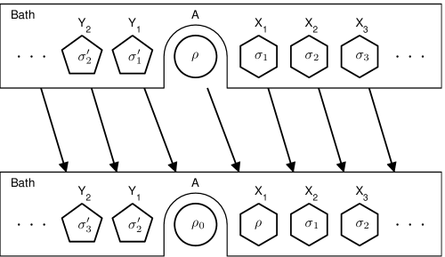
Figure 2: The isometry used in the realization for the complete erasure in the proof of the Theorem 2. The initial state in the top row is changed to the final state in the bottom row by copying the content of each subsystem to the next one on the right.

Let $\{\left|i\right\rangle\}$ and $\{\left|\alpha_{i}\right\rangle\}$ be the orthonormal sets in the Hilbert space of the device A that appear in the spectral decompositions of $Q$ and $\rho_{0}$ as in Eq. (29) and

$$\rho_{0}=\sum_{i=0}^{r-1}p_{i}\left|\alpha_{i}\right\rangle\left\langle\alpha_{i}\right|~{}~{}(p_{0}\geq p_{1}\geq\cdots\geq p_{r-1}>0)$$ (70)

where the eigenvalues are ordered in the indicated way. The isometry $U_{AB}$ on the composite system is defined as follows

$$U_{AB}\left|\ell\right\rangle_{A}\otimes\left|j_{1}j_{2}j_{3}\cdots;i_{1}i_{2}i_{3}\cdots\right\rangle_{B}=\left|\alpha_{j_{1}}\right\rangle_{A}\otimes\left|j_{2}j_{3}j_{4}\cdots;\ell i_{1}i_{2}\cdots\right\rangle_{B}~{}~{},$$ (71)

for any allowed values of input labels. Essentially, the isometry $U_{AB}$ shifts the contents of the device and the subsystems in a chain which is infinite in two directions. The movement of the information among the subsystems is depicted in Fig. 2. Specifically,

• the content of Y_k is copied to Y_k-1 for each $k\geq 2$,

• the content of Y₁ is copied to A in such a way that the standard basis of Y₁ is carried onto the eigenvectors of $\rho_{0}$,

• the content of A is copied to X₁ in such a way that the eigenvectors of $Q$ is carried onto the standard basis of X₁,

• and the content of X_k is copied onto X_k+1 for all $k$.

Note that $U_{AB}$ maps an orthonormal basis of AB to an orthonormal set and therefore it is an isometry.

For the Hamiltonian, the subsystems are taken to be independent and the Hamiltonians of individual subsystems are described in terms of a continuous parameter. For this purpose, consider continuous functions $\epsilon_{i}(\nu)$ ($i=0,1,\cdots,d-1$) and $\epsilon^{\prime}_{j}(\nu)$ ($j=0,1,\cdots,r-1$) of a real parameter $\nu\in[0,1]$, to be used for energies of X and Y type subsystems respectively. They are chosen to satisfy the following properties.

• The zeroth level has zero energy, $\epsilon_{0}(\nu)=\epsilon^{\prime}_{0}(\nu)=0$, for all $\nu$.

• The energies of all excited levels diverge to $+\infty$ as the corresponding parameter approaches to $1$, i.e.,

  $$\lim_{\nu\rightarrow 1}\epsilon_{i}(\nu)=\lim_{\nu\rightarrow 1}\epsilon^{\prime}_{j}(\nu)=\infty\quad(\textrm{for~{}any}~{}i,j\geq 1).$$ (72)

• The energy spectrum $\epsilon_{i}(\nu=0)$ is identical with the eigenvalues of $Q$ up to a constant shift as $\epsilon_{i}(0)=q_{i}-q_{0}$ for all $i$.

• The energy spectrum $\epsilon^{\prime}_{j}(\nu=0)$ is such that the equilibrium density matrix is isospectral with $\rho_{0}$, i.e., $\epsilon^{\prime}_{j}(0)=k_{B}T\ln(p_{0}/p_{j})$.

Let $\{\nu_{k}\}$ and $\{\nu^{\prime}_{k}\}$ be two infinite, increasing sequences starting from $0$ and converging to $1$. The energy levels of X_k and Y_k will be taken as $\epsilon_{i}(\nu_{k})$ and $\epsilon^{\prime}_{i}(\nu^{\prime}_{k})$ respectively. In other words, in terms of

$$h(\nu) = \sum_{i=0}^{d-1}\epsilon_{i}(\nu)\left|i\right\rangle\left\langle i\right|\quad,$$ (73)

$$h^{\prime}(\nu) = \sum_{i=0}^{r-1}\epsilon^{\prime}_{i}(\nu)\left|i\right\rangle\left\langle i\right|\quad,$$ (74)

the Hamiltonians of individual systems can be expressed as $H_{X_{k}}=h(\nu_{k})$ and $H_{Y_{k}}=h^{\prime}(\nu^{\prime}_{k})$. The bath Hamiltonian $H_{B}$ is the sum of the subsystem Hamiltonians and therefore the energy eigenvalue of the bath state $\left|j_{1}j_{2}\cdots;i_{1}i_{2}\cdots\right\rangle_{B}$ is

$$E(\{j_{k}\},\{i_{k}\})=\sum_{k=1}^{\infty}\epsilon^{\prime}_{j_{k}}(\nu_{k}^{\prime})+\epsilon_{i_{k}}(\nu_{k})~{}~{}~{}.$$ (75)

Let $\sigma(\nu)=\exp(-\beta h(\nu))/\zeta(\nu)$ and $\sigma^{\prime}(\nu)=\exp(-\beta h^{\prime}(\nu))/\zeta^{\prime}(\nu)$ be parameter-dependent density matrices and $\zeta(\nu)$ and $\zeta^{\prime}(\nu)$ be the corresponding partition functions. The shorthand notations $\sigma_{k}=\sigma(\nu_{k})$ and $\sigma^{\prime}_{k}=\sigma^{\prime}(\nu^{\prime}_{k})$ will be used for the states of X_k and Y_k respectively. The partition function of the bath is then given by

$$Z_{B}=\prod_{k=1}^{\infty}\zeta(\nu_{k})\zeta^{\prime}(\nu^{\prime}_{k})~{}~{}.$$ (76)

Depending only on the large $k$ behavior of the sequences $\{\nu_{k}\}$ and $\{\nu^{\prime}_{k}\}$, this product may converge or diverge.

In the following expressions, the subscripts are used for indicating the subsystem a given density matrix specifies to. Suppose that the initial state of the device A is $\rho$. The initial and final density matrices of the combined system are given by the following self-explanatory expressions.

$$\rho_{AB} = \cdots(\theta_{2})_{Y_{2}}\otimes(\theta_{1})_{Y_{1}}\otimes(\rho)_{A}\otimes(\sigma_{1})_{X_{1}}\otimes(\sigma_{2})_{X_{2}}\cdots$$

$$\rho_{AB}^{\prime} = \cdots(\theta_{3})_{Y_{2}}\otimes(\theta_{2})_{Y_{1}}\otimes(\rho_{0})_{A}\otimes(\rho)_{X_{1}}\otimes(\sigma_{1})_{X_{2}}\cdots$$

It is obvious that the reduced quantum operation on the device is $\mathcal{E}(\rho)=\rho_{0}$, i.e., the desired complete erasure. The change in the average energy of the bath is given by

$$\Delta E_{B}=\mathrm{tr}(\rho Q)-k_{B}T(J+S(\rho_{0}))+\Delta$$ (77)

where $J=J(\beta Q)$ and

$$\Delta = k_{B}T(J+S(\rho_{0}))-\mathrm{tr}\,\sigma_{1}Q+\sum_{k=2}^{\infty}\mathrm{tr}(\sigma_{k-1}-\sigma_{k})H_{X_{k}}$$ (78)

$$+\sum_{k=1}^{\infty}\mathrm{tr}(\sigma^{\prime}_{k+1}-\sigma^{\prime}_{k})H_{Y_{k}}~{}~{},$$

which is a constant independent of the device state $\rho$.

When Eq. (15) is used, $\Delta$ can be expressed as

$$\Delta=k_{B}T\sum_{k=1}^{\infty}\Big{(}S(\sigma_{k}||\sigma_{k+1})+S(\sigma^{\prime}_{k+1}||\sigma^{\prime}_{k})\Big{)}~{}~{},$$ (79)

which shows that $\Delta$ is a strictly positive number. It will be argued below that the sequences of subsystem parameters $\{\nu_{k}\}$ and $\{\nu^{\prime}_{k}\}$ can be selected in such a way that $\Delta$ can be adjusted to be equal to any positive value and this can be achieved with a finite $Z_{B}$. As in the proof of Theorem 3, this will be done by showing that $\Delta$ can be made arbitrarily large and arbitrarily small.

(1) First, if the parameter $\nu_{2}$ of X₂ tends to $1$, the final energy of X₂ approaches to infinity. In this limit $\Delta$ diverges to $\infty$. (ii) In the limit where all increments $\nu_{k+1}-\nu_{k}$ and $\nu^{\prime}_{k+1}-\nu^{\prime}_{k}$ tend to 0, the series in Eq. (78) approach to integrals which can readily be evaluated as in Eq. (61) and

$$\sum_{k=1}^{\infty}\mathrm{tr}(\sigma^{\prime}_{k+1}-\sigma^{\prime}_{k})H_{Y_{k}}\longrightarrow-k_{B}TS(\sigma^{\prime}(0))~{}~{}.$$ (80)

Therefore, in this limit, $\Delta$ approaches to $0$. This shows that $\Delta$ can be chosen as small as possible. It can also be shown that the same can be done with a finite $Z_{B}$ value.

Since $\Delta$ depends continuously on $\nu_{k}$ and $\nu^{\prime}_{k}$, it is then possible to adjust these parameter sequences such that $\Delta$ has the value

$$\Delta=k_{B}T(J+S(\rho_{0}))\quad,$$ (81)

which is a strictly positive quantity by our initial assumption. In that case, $\Delta E_{B}=\mathrm{tr}\,\rho Q$ and hence $Q$ is the HTO associated with this realization. This completes the proof of the Theorem 2. $\Box$

References

- (1) R. Landauer, IBM J. Res. Dev. 5, 183 (1961).
- (2) C. H. Bennett, Int. J. Theor. Phys. 21, 905 (1982).
- (3) O. Penrose, “Foundations of Statistical Mechanics”, (Pergamon Press, Oxford, 1970).
- (4) H.S. Leff and A.F. Rex, “Maxwell’s Demon 2: Entropy, Classical and Quantum Information, Computing”, (Institute of Physics, Bristol, 2003).
- (5) W. H. Zurek, in G.T. Moore and M. O. Scully, “Frontiers of Nonequilibrium Statistical Physics” (Plenum Press, New York, 1984); also reprinted in Ref. md2, .
- (6) S. LLoyd, Phys. Rev. A 56, 3374 (1997).
- (7) C. M. Bender, D. C. Brody and B. J. Meister, Proc. R. Soc. A 461, 733 (2005).
- (8) K. Shizume, Phys. Rev. E 52, 3495 (1995).
- (9) B. Piechocinska, Phys. Rev. A 61, 062314 (2000).
- (10) K. Jacobs, arXiv:quant-ph/0512105v1 (2005).
- (11) CAI Qing-Yu, Chin. Phys. Lett. 21, 1189 (2004).
- (12) O. J. E. Maroney, Studies in History and Philosophy of Modern Physics 36, 355 (2005).
- (13) O. J. E. Maroney, Phys. Rev. E 79, 031105 (2009).
- (14) S. Turgut, Phys. Rev. E 79, 041102 (2009).
- (15) N. G. Anderson, Phys. Lett. A 372, 5552 (2008).
- (16) T. Sagawa and M. Ueda, Phys. Rev. Lett. 102, 250602 (2009).
- (17) H.P. Breuer and F. Petruccione, “The theory of open quantum systems” (Oxford University Press, Oxford, 2002).
- (18) J. D. Norton, preprint available from http://www.pitt.edu/~jdnorton/papers/Waiting.pdf .
- (19) L. Szilard, Z. Phys. 53, 840 (1929).
- (20) P. Talkner, E. Lutz and P. Hänggi, Phys. Rev. E 75, 050102 (2007).
- (21) M. A. Nielsen and I. L. Chuang, Quantum Computation and Information (Cambridge University Press, Cambridge, 2000).
- (22) R. Bhatia, Positive Definite Matrices (Princeton University Press, Princeton and Oxford, 2007).