Divergences and Duality for Estimation and Test under Moment Condition Models

Abstract.

We introduce estimation and test procedures through divergence minimization for models satisfying linear constraints with unknown parameter. These procedures extend the empirical likelihood (EL) method and share common features with generalized empirical likelihood approach. We treat the problems of existence and characterization of the divergence projections of probability distributions on sets of signed finite measures. We give a precise characterization of duality, for the proposed class of estimates and test statistics, which is used to derive their limiting distributions (including the EL estimate and the EL ratio statistic) both under the null hypotheses and under alternatives or misspecification. An approximation to the power function is deduced as well as the sample size which ensures a desired power for a given alternative.
Keywords: Empirical likelihood; Generalized Empirical likelihood; Minimum divergence; Efficiency; Power function; Duality; Divergence projection.

1. Introduction and notation

Statistical models are often defined through estimating equations

$$\mathbb{E}\left[g(X,\theta)\right]=0,$$

where $\mathbb{E}[\cdot]$ denotes the mathematical expectation, $g:=(g_{1},\ldots,g_{l})^{\top}\in\mathbb{R}^{l}$ is some specified vector valued function of a random vector $X\in\mathbb{R}^{m}$ and a parameter vector $\theta\in\Theta\subset\mathbb{R}^{d}$. Examples of such models are numerous, see e.g. Qin and Lawless (1994), Haberman (1984), Sheehy (1987), McCullagh and Nelder (1983), Owen (2001) and the references therein. Denoting $M^{1}$ the collection of all probability measures (p.m.) on the measurable space $(\mathbb{R}^{m},\mathcal{B}(\mathbb{R}^{m}))$, the submodel $\mathcal{M}_{\theta}^{1}$, associated to a given value $\theta$ of the parameter, consists of all distributions $Q$ satisfying $l$ linear constraints induced by the vector valued function $g(.,\theta)$, namely

$$\mathcal{M}_{\theta}^{1}:=\left\{Q\in M^{1}~{}\text{ such that }~{}\int g(x,\theta)~{}dQ(x)=0\right\},$$

with $l\geq d$. The statistical model which we consider can be written as

$$\mathcal{M}^{1}:=\bigcup_{\theta\in\Theta}\mathcal{M}_{\theta}^{1}.$$ (1.1)

Let $X_{1},...,X_{n}$ denote an i.i.d sample of $X$ with unknown distribution $P_{0}$. We denote $\theta_{0}$, if it exists, the value of the parameter such that $P_{0}$ belongs to $\mathcal{M}_{\theta_{0}}^{1}$, namely the value satisfying

$$\mathbb{E}\left[g(X,\theta_{0})\right]=0,$$

and we assume obviously that $\theta_{0}$ is unique. This paper addresses the two following natural questions:

Problem 1: Does $P_{0}$ belong to the model $\mathcal{M}^{1}$?

Problem 2: When $P_{0}$ is in the model, which is the value $\theta_{0}$ of the parameter for which $\mathbb{E}\left[g(X,\theta_{0})\right]=0$? Also can we perform tests about $\theta_{0}$? Can we construct confidence areas for $\theta_{0}$?

We note that these problems have been investigated by many authors. Hansen (1982) considered generalized method of moments (GMM). Hansen et al. (1996) introduced the continuous updating (CU) estimate. The empirical likelihood (EL) approach, developed by Owen (1988) and Owen (1990), has been investigated in the context of model (1.1) by Qin and Lawless (1994) and Imbens (1997) introducing the EL estimate. The recent literature in econometrics focusses on such models; Smith (1997), Newey and Smith (2004) provided a class of estimates called generalized empirical likelihood (GEL) estimates which contains the EL and the CU ones. Schennach (2007) discussed the asymptotic properties of the empirical likelihood estimate under misspecification; the author showed the important fact that the EL estimate may cease to be root $n$ consistent when the functions $g_{j}$ defining the moments conditions and the support of $P_{0}$ are unbounded. Among other results pertaining to EL, Newey and Smith (2004) stated that EL estimate enjoys optimality properties in term of efficiency when bias corrected among all GEL estimates including the GMM one. Moreover, Corcoran (1998) and Baggerly (1998) proved that in a class of minimum discrepancy statistics (called power divergence statistics), EL ratio is the only one that is Bartlett correctable. Confidence areas for the parameter $\theta_{0}$ have been considered in the seminal paper by Owen (1990). Problems 1 and 2 have been handled via EL and GEL approaches in Qin and Lawless (1994), Smith (1997) and Newey and Smith (2004) under the null hypothesis $\mathcal{H}_{0}:P_{0}\in\mathcal{M}^{1}$; the limiting distributions of the GEL estimates and the GEL test statistics have been obtained under the model and under the null hypotheses. Imbens (1997) discusses the asymptotic properties of the EL and exponential tilting estimates under misspecification and give the formula of the asymptotic variance, using dual characterizations, without presenting the hypotheses under which their results hold. Chen et al. (2007) give the limiting distribution of the EL estimate under misspecification as well as the EL ratio statistic between a parametric model and a moment condition model. The paper by Kitamura (2007) gives a discussion of duality for GEL estimates under moment condition models. Bertail (2006) uses duality to study, under the model, the asymptotic properties of the EL ratio statistic and its Bartlett correctability; the author extends his results to semiparametric problems with infinite-dimensional parameters.

The main contribution of the present paper is the precise characterization of duality for a large class of estimates and test statistics (including GEL and EL ones) and its use in deriving the limiting properties of both the estimates and the test statistics under misspecification and under alternatives hypotheses. Moreover,

1. The approach which we develop is based on minimum discrepancy estimates, which extends the EL method and has common features with minimum distance and GEL techniques, using merely divergences. We present a wide class of estimates, test statistics and confidence regions for the parameter $\theta_{0}$ as well as various test statistics for Problems 1 and 2, all depending on the choice of the divergence.
   

2. The limiting distribution of the EL test statistic under the alternative and under misspecification remains up to date an open problem. The present paper fills this gap; indeed, we give the limiting distributions of the proposed estimates and test statistics (including the EL ones) both under the null hypotheses, under alternatives and under misspecification.
   

3. The limiting distributions of the test statistics under the alternatives and misspecification are used to give an approximation to the power function and the sample size which ensures a desired power for a given alternative.
   

4. We extend confidence region (C.R.) estimation techniques based on EL (see Owen (1990)), providing a wide range of such C.R.’s, each one depending upon a specific divergence.

From the point of view of the statistical criterion under consideration, the main advantage, of using a divergence based approach and duality, lays in the fact that it leads to asymptotic properties of the estimates and test statistics under the alternative, including misspecification, which cannot be achieved through the classical EL context. In the case of parametric models of densities, White (1982) studied the asymptotic properties of the parametric maximum likelihood estimate and the parametric likelihood ratio statistic under misspecification; Keziou (2003) and Broniatowski and Keziou (2009) stated the consistency and obtained the limiting distributions of the minimum divergence estimates and the corresponding test statistics (including the parametric likelihood ones) both under the null hypotheses and the alternatives, from which they deduced an approximation to the power function. In this paper, we extend the above results for the proposed class of estimates and test statistics (including the EL ones) in the context of semiparametric models (1.1).

The rest of the paper is organized as follows. Section 2 describes the statistical divergences used in the sequel. Section 3 is devoted to the description of the proposed estimation and test procedures. In Section 3, we adapt the Lagrangian duality formalism to the context of statistical divergence, and we use it to give practical formulas (for the study and the numerical computation) of the proposed estimates and test statistics. Section 5 deals with the asymptotic properties of the estimates and the test statistics under the model and under misspecification. Simulations results are given in Section 6. All proofs are postponed to the Appendix.

2. Statistical divergences

We first set some general definitions and notations. Let $P$ be some p.m. on the measurable space $(\mathbb{R}^{m},\mathcal{B}(\mathbb{R}^{m}))$. Denote by $M$ the space of all signed finite measures (s.f.m.) on $(\mathbb{R}^{m},\mathcal{B}(\mathbb{R}^{m}))$. Let $\varphi$ be a convex function from $\mathbb{R}$ onto $[0,+\infty]$ with $\varphi(1)=0$, and such that its domain, $\text{dom}\varphi:=\left\{x\in\mathbb{R}\text{ such that }\varphi(x)<\infty\right\}=:(a,b),$ is an interval, with endpoints $a<1<b$, which may be bounded or unbounded, open or not. We assume that $\varphi$ is closed. For any s.f.m. $Q\in M$, the $\varphi$-divergence between $Q$ and the p.m. $P$, when $Q$ is absolutely continuous with respect to (a.c.w.r.t) $P$, is defined through

$$D_{\varphi}(Q,P):=\int_{\mathbb{R}^{m}}\varphi\left(\frac{dQ}{dP}(x)\right)~{}dP(x),$$ (2.1)

in which $\frac{dQ}{dP}(\cdot)$ denotes the Radon-Nikodym derivative. When $Q$ is not a.c.w.r.t. $P$, we set $D_{\varphi}(Q,P):=+\infty$. For any p.m. $P$, the mapping $Q\in M\mapsto D_{\varphi}(Q,P)$ is convex and takes nonnegative values. When $Q=P$ then $D_{\varphi}(Q,P)=0$. Furthermore, if the function $x\mapsto\varphi(x)$ is strictly convex on a neighborhood of $x=1$, then

$$D_{\varphi}(Q,P)=0~{}\text{ if and only if }~{}Q=P.$$ (2.2)

All the above properties are presented in Csiszár (1963), Csiszár (1967) and in Chapter 1 of Liese and Vajda (1987), for $\varphi-$divergences defined on the set of all p.m.’s $M^{1}$. When the $\varphi$-divergences are extended to $M$, then the same arguments as developed on $M^{1}$ hold. When defined on $M^{1}$, the Kullback-Leibler $(KL)$, modified Kullback-Leibler $(KL_{m})$, $\chi^{2}$, modified $\chi^{2}$ $(\chi_{m}^{2})$, Hellinger $(H)$, and $L^{1}$ divergences are respectively associated to the convex functions $\varphi(x)=x\log x-x+1$, $\varphi(x)=-\log x+x-1$, $\varphi(x)=\frac{1}{2}{(x-1)}^{2}$, $\varphi(x)=\frac{1}{2}{(x-1)}^{2}/x$, $\varphi(x)=2{(\sqrt{x}-1)}^{2}$ and $\varphi(x)=\left|x-1\right|$. All these divergences except the $L^{1}$ one, belong to the class of the so called power divergences introduced in Cressie and Read (1984) (see also Liese and Vajda (1987) and Pardo (2006)). They are defined through the class of convex functions

$$x\in\mathbb{R}_{+}^{\ast}\mapsto\varphi_{\gamma}(x):=\frac{x^{\gamma}-\gamma x+\gamma-1}{\gamma(\gamma-1)}$$ (2.3)

if $\gamma\in\mathbb{R}\setminus\left\{0,1\right\}$, $\varphi_{0}(x):=-\log x+x-1$ and $\varphi_{1}(x):=x\log x-x+1$. So, the $KL-$divergence is associated to $\varphi_{1}$, the $KL_{m}$ to $\varphi_{0}$, the $\chi^{2}$ to $\varphi_{2}$, the $\chi_{m}^{2}$ to $\varphi_{-1}$ and the Hellinger distance to $\varphi_{1/2}$. We extend the definition of the power divergences functions $Q\in M^{1}\mapsto D_{\varphi_{\gamma}}(Q,P)$ onto the whole set of signed finite measures $M$ as follows. When the function $x\mapsto\varphi_{\gamma}(x)$ is not defined on $]-\infty,0[$ or when $\varphi_{\gamma}$ is defined on $\mathbb{R}$ but is not convex, we extend the definition of $\varphi_{\gamma}$ as follows

$$x\in\mathbb{R}\mapsto\varphi_{\gamma}(x)\mathds{1}_{[0,+\infty[}(x)+(+\infty)\mathds{1}_{]-\infty,0[}(x).$$ (2.4)

Note that for $\chi^{2}$-divergence, the corresponding $\varphi$ function $\varphi(x)=\frac{1}{2}(x-1)^{2}$ is convex and defined on whole $\mathbb{R}$. In this paper, for technical considerations, we assume that the functions $\varphi$ are strictly convex on their domain $(a,b)$, twice continuously differentiable on $]a,b[$, the interior of their domain. Hence, $\varphi^{\prime}(1)=0$, and for all $x\in]a,b[$, $\varphi^{\prime\prime}(x)>0$. Here, $\varphi^{\prime}$ and $\varphi^{\prime\prime}$ are used to denote respectively the first and the second derivative functions of $\varphi$. Moreover, we assume that $\varphi$ is “essentially smooth” in the sense that $\lim_{x\downarrow a}\varphi^{\prime}(x)=-\infty$ if $a$ is finite and $\lim_{x\uparrow b}\varphi^{\prime}(x)=+\infty$ if $b$ is finite. Note that the above assumptions on $\varphi$ are not restrictive, and that all the power functions $\varphi_{\gamma}$, see (2.4), satisfy the above conditions, including all standard divergences.

Definition 2.1.

Let $\Omega$ be some subset of $M$. The $\varphi-$divergence between the set $\Omega$ and a p.m. $P$ is defined by

$$D_{\varphi}(\Omega,P):=\inf_{Q\in\Omega}D_{\varphi}(Q,P).$$

A finite measure $Q^{\ast}\in\Omega$, such that $D_{\varphi}(Q^{\ast},P)<\infty$ and

$$D_{\varphi}(Q^{\ast},P)\leq D_{\varphi}(Q,P)~{}\text{ for all }~{}Q\in\Omega,$$

is called a projection of $P$ on $\Omega$. This projection may not exist, or may be not defined uniquely.

3. Minimum divergence estimates

Let $X_{1},...,X_{n}$ denote an i.i.d. sample of a random vector $X\in\mathbb{R}^{m}$ with distribution $P_{0}$. Let $P_{n}$ be the empirical measure pertaining to this sample, namely

$$P_{n}:=\frac{1}{n}\sum_{i=1}^{n}\delta_{X_{i}},$$

where $\delta_{x}$ denotes the Dirac measure at point $x$, for all $x$. We will endow our statistical approach in the global context of s.f.m’s with total mass $1$ satisfying $l$ linear constraints:

$$\mathcal{M}_{\theta}:=\left\{Q\in M~{}\text{ such that }~{}\int_{\mathbb{R}^{m}}dQ(x)=1\text{ and }\int_{\mathbb{R}^{m}}g(x,\theta)~{}dQ(x)=0\right\}$$ (3.1)

and

$$\mathcal{M}:=\bigcup_{\theta\in\Theta}\mathcal{M}_{\theta},$$ (3.2)

sets of signed finite measures that replace $\mathcal{M}_{\theta}^{1}$ and $\mathcal{M}^{1}$. Enhancing the model (1.1) to the above one (3.2) bears a number of improvements upon existing results; this is argued at the end of the present Section; see also Remark 4.5 below. The “plug-in” estimate of $D_{\varphi}(\mathcal{M}_{\theta},P_{0})$ is

$$\widehat{D}_{\varphi}(\mathcal{M}_{\theta},P_{0}):=\inf_{Q\in\mathcal{M}_{\theta}}D_{\varphi}(Q,P_{n})=\inf_{Q\in\mathcal{M}_{\theta}}\int_{\mathbb{R}^{m}}\varphi\left(\frac{dQ}{dP_{n}}(x)\right)~{}dP_{n}(x).$$ (3.3)

If the projection $Q^{(n)}_{\theta}$ of $P_{n}$ on $\mathcal{M}_{\theta}$ exists, then it is clear that $Q^{(n)}_{\theta}$ is a s.f.m. (or possibly a p.m.) a.c.w.r.t. $P_{n}$; this means that the support of $Q^{(n)}_{\theta}$ must be included in the set $\left\{X_{1},\ldots,X_{n}\right\}$. So, define the sets

$$\mathcal{M}_{\theta}^{(n)}:=\left\{Q\in M~{}|~{}Q\text{ a.c.w.r.t. }P_{n},~{}\sum_{i=1}^{n}Q(X_{i})=1\text{ and }\sum_{i=1}^{n}Q(X_{i})g(X_{i},\theta)=0\right\},$$ (3.4)

which may be seen as subsets of $\mathbb{R}^{n}$. Then, the plug-in estimate (3.3) can be written as

$$\widehat{D}_{\varphi}(\mathcal{M}_{\theta},P_{0})=\inf_{Q\in\mathcal{M}_{\theta}^{(n)}}\frac{1}{n}\sum_{i=1}^{n}\varphi\left(nQ(X_{i})\right).$$ (3.5)

In the same way, $D_{\varphi}(\mathcal{M},P_{0}):=\inf_{\theta\in\Theta}\inf_{Q\in\mathcal{M}_{\theta}}D_{\varphi}(Q,P_{0})$ can be estimated by

$$\widehat{D}_{\varphi}(\mathcal{M},P_{0}):=\inf_{\theta\in\Theta}\inf_{Q\in\mathcal{M}_{\theta}^{(n)}}\frac{1}{n}\sum_{i=1}^{n}\varphi\left(nQ(X_{i})\right).$$ (3.6)

By uniqueness of $\arg\inf_{\theta\in\Theta}D_{\varphi}(\mathcal{M}_{\theta},P_{0})$ and since the infimum is reached at $\theta=\theta_{0}$ under the model, we estimate $\theta_{0}$ through

$$\widehat{\theta}_{\varphi}:=\arg\inf_{\theta\in\Theta}\inf_{Q\in\mathcal{M}_{\theta}^{(n)}}\frac{1}{n}\sum_{i=1}^{n}\varphi\left(nQ(X_{i})\right).$$ (3.7)

Enhancing $\mathcal{M}^{1}$ to $\mathcal{M}$ and accordingly extensions in the definitions of the $\varphi$ functions on $\mathbb{R}$ and the $\varphi$-divergences on the whole space of s.f.m’s $M$, is motivated by the following arguments:

1. If the domain $(a,b)$ of the function $\varphi$ is included in $[0,+\infty[$ then minimizing over $\mathcal{M}^{1}$ or over $\mathcal{M}$ leads to the same estimates and test statistics. It is the case of the $KL_{m}$, $KL$, modified $\chi^{2}$ and Hellinger divergences.

2. Let $\theta$ be a given value in $\Theta$. Denote $Q^{(1,n)}_{\theta}$ and $Q^{(n)}_{\theta}$, respectively, the projection of $P_{n}$ on $\mathcal{M}_{\theta}^{1}$ and on $\mathcal{M}_{\theta}$. If $Q^{(1,n)}_{\theta}$ satisfies $0<Q^{(1,n)}_{\theta}(X_{i})<1$, for all $i=1,\ldots,n,$ then $Q^{(1,n)}_{\theta}=Q^{(n)}_{\theta}$. Therefore, in this case, both approaches leads also to the same estimates and test statistics.

3. It may occur that for some $\theta$ in $\Theta$ and some $i=1,\ldots,n,$ $Q^{(1,n)}_{\theta}(X_{i})$ is a boundary value of $[0,1]$, hence the first order conditions are not met which makes a real difficulty for the calculation of the estimates over the sets of p.m. $\mathcal{M}^{1}_{\theta}$ and $\mathcal{M}^{1}$. However, when $\mathcal{M}^{1}$ is replaced by $\mathcal{M}$, then this problem does not hold any longer in particular when $\text{dom}\varphi=\mathbb{R}$, which is the case for the $\chi^{2}$-divergence. Other arguments are given in Remark 4.5 below.

The empirical likelihood paradigm (see Owen (1988), Owen (1990), Qin and Lawless (1994) and Owen (2001)), enters as a special case of the statistical issues related to estimation and tests based on $\varphi-$divergences with $\varphi(x)=\varphi_{0}(x):=-\log x+x-1$, namely on $KL_{m}-$divergence. Indeed, it is straightforward to see that the empirical log-likelihood ratio statistic for testing $\mathcal{H}_{0}:P_{0}\in\mathcal{M}$ against $\mathcal{H}_{1}:P_{0}\notin\mathcal{M}$, in the context of $\varphi$-divergences, can be written as $2n\widehat{D}_{KL_{m}}(\mathcal{M},P_{0})$; and that the EL estimate of $\theta_{0}$ can be written as $\widehat{\theta}_{KL_{m}}=\arg\inf_{\theta\in\Theta}\widehat{D}_{KL_{m}}(\mathcal{M}_{\theta},P_{0})$; see Remark 4.3 below. In the case of the power functions $\varphi=\varphi_{\gamma}$, the corresponding estimates (3.7) belong to the class of GEL estimates introduced by Smith (1997) and Newey and Smith (2004), and (3.5) in this case are the empirical Cressie-Read statistics introduced by Baggerly (1998) and Corcoran (1998); see Remark 4.4 below.

The constrained optimization problems (3.5), (3.6) and (3.7) can be transformed into unconstrained ones making use of some arguments of “duality” which we briefly state below from Rockafellar (1970). On the other hand, the obtaining of asymptotic statistical results of the estimates and the test statistics, under misspecification or under alternative hypotheses, requires handle existence conditions and characterization of the projection of $P_{0}$ on the submodel $\mathcal{M}_{\theta}$ or on the model $\mathcal{M}.$ This also will be considered through duality, along the following Section.

4. Dual representation of $\varphi-$divergences under constraints

This Section is central for our purposes. Indeed, it provides the explicit form of the proposed estimates by transforming the constrained problems (3.5) to unconstrained ones, using Lagrangian duality which is a classical tool in optimization theory. This Section adapts this formalism to the context of divergences and the present statistical setting. The Lagrangian “dual” problem, corresponding to the “primal” one

$$\inf_{Q\in\mathcal{M}_{\theta}}D_{\varphi}(Q,P_{0})$$ (4.1)

and its empirical counterpart (3.5), make use of the so-called Fenchel-Legendre transform of $\varphi$, defined through

$$\psi:t\in\mathbb{R}\mapsto\psi(t):=\sup_{x\in\mathbb{R}}\left\{tx-\varphi(x)\right\}.$$ (4.2)

The “dual” problems associated to $(\ref{Primal theo})$ and (3.5) are respectively

$$\sup_{t\in\mathbb{R}^{1+l}}\left\{t_{0}-\int_{\mathbb{R}^{m}}\psi(t_{0}+\sum_{j=1}^{l}t_{j}g_{j}(x,\theta))~{}dP_{0}(x)\right\},$$ (4.3)

and

$$\sup_{t\in\mathbb{R}^{1+l}}\left\{t_{0}-\frac{1}{n}\sum_{i=1}^{n}\psi(t_{0}+\sum_{j=1}^{l}t_{j}g_{j}(X_{i},\theta))\right\}.$$ (4.4)

In the following Propositions 4.1 and 4.2, we state sufficient conditions under which the primal problems (4.1) and (3.5) coincide respectively with the dual ones (4.3) and (4.4). First, recall some properties of the convex conjugate $\psi$ of $\varphi$. For the proofs, we can refer to Section 26 in Rockafellar (1970). The function $\psi$ is convex and closed, its domain is an interval with endpoints

$$a^{*}:=\lim_{x\to-\infty}\frac{\varphi(x)}{x},\quad b^{*}:=\lim_{x\to+\infty}\frac{\varphi(x)}{x}$$ (4.5)

satisfying $a^{*}<0<b^{*}$ with $\psi(0)=0$. The strict convexity of $\varphi$ on its domain $(a,b)$ is equivalent to the condition that its conjugate $\psi$ is essentially smooth, i.e., differentiable with

$$\begin{array}[c]{ccccc}\lim_{t\downarrow a^{*}}{\psi}^{\prime}(t)&=&-\infty&\text{ if }&a^{*}\text{ is finite},\\ \lim_{t\uparrow b^{*}}{\psi}^{\prime}(t)&=&+\infty&\text{ if }&b^{*}\text{ is finite}.\end{array}$$ (4.6)

Conversely, $\varphi$ is essentially smooth on its domain $(a,b)$ if and only if $\psi$ is strictly convex on its domain $(a^{*},b^{*})$. In all the sequel, we assume additionally that $\varphi$ is essentially smooth. Hence, $\psi$ is strictly convex on its domain $(a^{*},b^{*})$, and it holds that

$$a^{*}=\lim_{x\downarrow a}\varphi^{\prime}(x),\quad\quad b^{*}=\lim_{x\uparrow b}\varphi^{\prime}(x),$$

and

$$\psi(t)=t{\varphi^{\prime}}^{-1}(t)-\varphi\left({\varphi^{\prime}}^{-1}(t)\right),\quad\text{for all }t\in]a^{*},b^{*}[,$$ (4.7)

where ${\varphi^{\prime}}^{-1}$ denotes the inverse function of $\varphi^{\prime}$. It holds also that $\psi$ is twice continuously differentiable on $]a^{*},b^{*}[$ with

$$\psi^{\prime}(t)={\varphi^{\prime}}^{-1}(t)\quad\text{and}\quad\psi^{\prime\prime}(t)=\frac{1}{\varphi^{\prime\prime}\left({\varphi^{\prime}}^{-1}(t)\right)}.$$ (4.8)

In particular, $\psi^{\prime}(0)=1$ and $\psi^{\prime\prime}(0)=1$. Obviously, since $\varphi$ is assumed to be closed, we have

$$\varphi(a)=\lim_{x\downarrow a}\varphi(x)\quad\text{ and }\quad\varphi(b)=\lim_{x\uparrow b}\varphi(x),$$

which may be finite or infinite. Hence, by closedness of $\psi$, we have

$$\psi(a^{*})=\lim_{t\downarrow a^{*}}\psi(x)\quad\text{ and }\quad\psi(b^{*})=\lim_{t\uparrow b^{*}}\psi(t).$$

Finally, the first and second derivatives of $\varphi$ in $a$ and $b$ are defined to be the limits of $\varphi^{\prime}(x)$ and $\varphi^{\prime\prime}(x)$ when $x\downarrow a$ and when $x\uparrow b$. The first and second derivatives of $\psi$ in $a^{*}$ and $b^{*}$ are defined in a similar way. In Table 1, we give the convex conjugates $\psi$ of some standard functions $\varphi$, associated to some standard divergences. We determine also their domains, $(a,b)$ and $(a^{*},b^{*})$.

Table 1. Convex conjugates for some standard divergences.

$D_{\varphi}$	$\varphi$	$\text{dom}\varphi$	$\text{dom}\psi$	$\psi$
$D_{KL_{m}}$	$\varphi(x):=-\log x+x-1$	$]0,+\infty[$	$]-\infty,1[$	$\psi(t)=-\log(1-t)$
$D_{KL}$	$\varphi(x):=x\log x-x+1$	$[0,+\infty[$	$\mathbb{R}$	$\psi(t)=e^{t}-1$
$D_{\chi^{2}_{m}}$	$\varphi(x):=\frac{1}{2}\frac{\left(x-1\right)^{2}}{x}$	$]0,+\infty[$	$\left]-\infty,\frac{1}{2}\right]$	$\psi(t)=1-\sqrt{1-2t}$
$D_{\chi^{2}}$	$\varphi(x):=\frac{1}{2}\left(x-1\right)^{2}$	$\mathbb{R}$	$\mathbb{R}$	$\psi(t)=\frac{1}{2}t^{2}+t$
$D_{H}$	$\varphi(x):=2(\sqrt{x}-1)^{2}$	$[0,+\infty[$	$]-\infty,2[$	$\psi(t)=\frac{2t}{2-t}$
$D_{\varphi_{\gamma}}$	$\varphi(x):=\frac{x^{\gamma}-\gamma x+\gamma-1}{\gamma(\gamma-1)}$	$--$	$--$	$\psi(t)=\frac{1}{\gamma}\left(\gamma t-t+1\right)^{\frac{\gamma}{\gamma-1}}-\frac{1}{\gamma}$

Proposition 4.1.

Let $\theta$ be a given value in $\Theta$. If there exists $Q_{0}$ in $\mathcal{M}_{\theta}^{(n)}$ such that

$$a<Q_{0}(X_{i})<b,\quad\text{for all}\quad i=1,\ldots,n,$$ (4.9)

then

$$\inf_{Q\in\mathcal{M}_{\theta}^{(n)}}D_{\varphi}(Q,P_{n})=\sup_{t\in\mathbb{R}^{1+l}}\left\{t_{0}-\frac{1}{n}\sum_{i=1}^{n}\psi(t_{0}+\sum_{j=1}^{l}t_{j}g_{j}(X_{i},\theta))\right\}$$ (4.10)

with dual attainment. Conversely, if there exists some dual optimal solution $\widehat{t}:=(\widehat{t}_{0},\widehat{t}_{1},\ldots,\widehat{t}_{l})^{\top}\in\mathbb{R}^{1+l}$ such that

$$a^{*}<\widehat{t_{0}}+\sum_{j=1}^{l}\widehat{t_{j}}g_{j}(X_{i},\theta)<b^{*},\quad\text{for all}\quad i=1,\ldots,n,$$ (4.11)

then the equality (4.10) holds, and the unique optimal solution of the primal problem $\inf_{Q\in\mathcal{M}_{\theta}^{(n)}}D_{\varphi}(Q,P_{n})$, namely the projection of $P_{n}$ on $\mathcal{M}^{(n)}_{\theta}$, is given by

$$Q^{(n)}_{\theta}(X_{i})=\frac{1}{n}{\varphi^{\prime}}^{-1}(\widehat{t_{0}}+\sum_{j=1}^{l}\widehat{t_{j}}g_{j}(X_{i},\theta)),\quad i=1,\ldots,n,$$

where $\widehat{t}:=(\widehat{t}_{0},\widehat{t}_{1},\ldots,\widehat{t}_{l})^{\top}$ is solution of the system of equations

$$\left\{\begin{array}[]{lll}1-\frac{1}{n}\sum_{i=1}^{n}{\varphi^{\prime}}^{-1}(\widehat{t_{0}}+\sum_{j=1}^{l}\widehat{t_{j}}g_{j}(X_{i},\theta))&=&0,\\ -\frac{1}{n}\sum_{i=1}^{n}g_{j}(X_{i},\theta){\varphi^{\prime}}^{-1}(\widehat{t_{0}}+\sum_{j=1}^{l}\widehat{t_{j}}g_{j}(X_{i},\theta))&=&0,\quad j=1,\ldots,l.\\ \end{array}\right.$$

Remark 4.1.

For the $\chi^{2}-$divergence, we have $a=-\infty$ and $b=+\infty$. Hence, condition (4.9) holds whenever $\mathcal{M}_{\theta}^{(n)}$ is not void. More generally, the above Proposition holds for any $\varphi$-divergence with $\text{dom}\varphi=\mathbb{R}$.

Remark 4.2.

Assume that $g(x,\theta):=(x-\theta)^{\top}$. So, for any divergence $D_{\varphi}$ with $\text{dom}\varphi=]0,+\infty[$, which is the case of the modified $\chi^{2}$ divergence and the modified Kullback-Leibler divergence (or equivalently EL method), condition $(\ref{cond Owen})$ means that $\theta$ is an interior point of the convex hull of the data $(X_{1},...,X_{n})$. This is precisely what is checked in Owen (1990), p. 100, for the EL method; see also Owen (2001).

For the asymptotic counterpart of the above results we have; see Theorem 1 in Broniatowski and Keziou (2006):

Proposition 4.2.

Let $\theta$ be a given value in $\Theta$. Assume that $\int|g_{j}(x,\theta)|~{}dP_{0}(x)<\infty$, for all $j=1,\ldots,l$. If there exists $Q_{0}$ in $\mathcal{M}_{\theta}$ with $D_{\varphi}(Q_{0},P_{0})<\infty$ and

$$a<\inf_{x\in\mathbb{R}^{m}}\frac{dQ_{0}}{dP_{0}}(x)\leq\sup_{x\in\mathbb{R}^{m}}\frac{dQ_{0}}{dP_{0}}(x)<b,\quad P_{0}-a.s.,$$ (4.12)

then

$$\inf_{Q\in\mathcal{M}_{\theta}}D_{\varphi}(Q,P_{0})=\sup_{t\in\mathbb{R}^{1+l}}\left\{t_{0}-\int_{\mathbb{R}^{m}}\psi(t_{0}+\sum_{j=1}^{l}t_{j}g_{j}(x,\theta))~{}dP_{0}(x)\right\}$$ (4.13)

with dual attainment. Conversely, if there exists some dual optimal solution $t^{*}$ which is an interior point of the set

$$\left\{t\in\mathbb{R}^{1+l}~{}\text{such that}~{}\int_{\mathbb{R}^{m}}|\psi(t_{0}+\sum_{j=1}^{l}t_{j}g_{j}(x,\theta))|~{}dP_{0}(x)<\infty\right\},$$ (4.14)

then the dual equality (4.13) holds, and the unique optimal solution $Q^{*}_{\theta}$ of the primal problem $\inf_{Q\in\mathcal{M}_{\theta}}D_{\varphi}(Q,P_{0})$, namely the projection of $P_{0}$ on $\mathcal{M}_{\theta}$, is given by

$$\frac{dQ^{*}_{\theta}}{dP_{0}}(x)={\varphi^{\prime}}^{-1}(t_{0}^{*}+\sum_{j=1}^{l}t_{j}^{*}g_{j}(x,\theta)),$$

where $t^{*}:=(t^{*}_{0},t^{*}_{1},\ldots,t^{*}_{l})^{\top}$ is solution of the system of equations

$$\left\{\begin{array}[]{lll}1-\int{\varphi^{\prime}}^{-1}(t_{0}^{*}+\sum_{j=1}^{l}t_{j}^{*}g_{j}(x,\theta))~{}dP_{0}(x)&=&0,\\ -\int g_{j}(x,\theta){\varphi^{\prime}}^{-1}(t_{0}^{*}+\sum_{j=1}^{l}t_{j}^{*}g_{j}(x,\theta))~{}dP_{0}(x)&=&0,\quad j=1,\ldots,l.\\ \end{array}\right.$$ (4.15)

Furthermore, $t^{*}$ is unique if the functions $\mathds{1}_{\mathbb{R}^{m}},g_{1}(.,\theta),\ldots,g_{l}(.,\theta)$ are linearly independent in the sense that $P_{0}\left\{x\in\mathbb{R}^{m}~{}|~{}t_{0}+\sum_{j=1}^{l}t_{j}g_{j}(x,\theta)\neq 0\right\}>0$ for all $t\in\mathbb{R}^{m}$ with $t\neq 0.$

For sake of brevity and clearness, we must introduce some additional notations. In all the sequel, $\|x\|$ denotes the norm of $x$ defined by $\|x\|:=\sup_{i}|x_{i}|$ for any vector $x:=(x_{1},\ldots,x_{k})^{\top}\in\mathbb{R}^{k}$, and for any matrix $A$, the norm of $A$ is defined by $\|A\|:=\sup_{i,j}|a_{i,j}|$. Denote by $\overline{g}$ the vector valued function $\overline{g}:=(\mathds{1}_{\mathbb{R}^{m}},g_{1},\ldots,g_{l})^{\top}\in\mathbb{R}^{1+l}$. For any p.m. $P$ on $(\mathbb{R}^{m},\mathcal{B}(\mathbb{R}^{m}))$ and any real measurable function $f$ from $(\mathbb{R}^{m},\mathcal{B}(\mathbb{R}^{m}))$ to $(\mathbb{R},\mathcal{B}(\mathbb{R}))$, denote

$$Pf:=\int_{\mathbb{R}^{m}}f(x)~{}dP(x).$$

Let

$$t^{\top}\overline{g}(x,\theta):=t_{0}+\sum_{j=1}^{l}t_{j}g_{j}(x,\theta)$$

and

$$m(x,\theta,t):=t_{0}-\psi(t^{\top}\overline{g}(x,\theta)),\text{ for all }x\in\mathbb{R}^{m},\theta\in\Theta\subset\mathbb{R}^{d},t\in\mathbb{R}^{1+l}.$$ (4.16)

Note that the $\sup$ in (4.10) and (4.13) can be restricted, respectively, to the sets

$$\Lambda_{\theta}^{(n)}:=\left\{t\in\mathbb{R}^{1+l}~{}|~{}a^{*}<t^{\top}\overline{g}(X_{i},\theta)<b^{*},~{}\text{ for all }i=1,\ldots,n\right\}$$ (4.17)

and

$$\Lambda_{\theta}:=\left\{t\in\mathbb{R}^{1+l}~{}|~{}\int_{\mathbb{R}^{m}}|\psi(t_{0}+\sum_{j=1}^{l}t_{j}g_{j}(x,\theta))|~{}dP_{0}(x)<\infty\right\}.$$ (4.18)

In view of the above two Propositions 4.1 and 4.2, we redefine the estimates (3.5), (3.6) and (3.7) as follows

$$\widehat{D}_{\varphi}\left(\mathcal{M}_{\theta},P_{0}\right):=\sup_{t\in\Lambda_{\theta}^{(n)}}\frac{1}{n}\sum_{i=1}^{n}m(X_{i},\theta,t):=\sup_{t\in\Lambda_{\theta}^{(n)}}P_{n}m(\theta,t),$$ (4.19)

$$\widehat{D}_{\varphi}\left(\mathcal{M},P_{0}\right):=\inf_{\theta\in\Theta}\sup_{t\in\Lambda_{\theta}^{(n)}}\frac{1}{n}\sum_{i=1}^{n}m(X_{i},\theta,t):=\inf_{\theta\in\Theta}\sup_{t\in\Lambda_{\theta}^{(n)}}P_{n}m(\theta,t)$$ (4.20)

and

$$\widehat{\theta}_{\varphi}:=\arg\inf_{\theta\in\Theta}\sup_{t\in\Lambda_{\theta}^{(n)}}\frac{1}{n}\sum_{i=1}^{n}m(X_{i},\theta,t):=\arg\inf_{\theta\in\Theta}\sup_{t\in\Lambda_{\theta}^{(n)}}P_{n}m(\theta,t).$$ (4.21)

Remark 4.3.

When $\varphi(x)=-\log x+x-1$, then the estimate (3.7) clearly coincides with the EL one, so it can be seen as the value of the parameter which minimizes the $KL_{m}$-divergence between the model $\mathcal{M}$ and the empirical measure $P_{n}$ of the data $X_{1},\ldots,X_{n}$. The statistic $2n\widehat{D}_{KL_{m}}(\mathcal{M},P_{0})$, see (3.6), coincides with the empirical likelihood ratio statistic associated to the null hypothesis $\mathcal{H}_{0}:P_{0}\in\mathcal{M}$ against the alternative $\mathcal{H}_{1}:P_{0}\not\in\mathcal{M}$. The dual representation of $\widehat{D}_{KL_{m}}(\mathcal{M},P_{0})$, see (4.20) and (4.10), is

$$\widehat{D}_{KL_{m}}(\mathcal{M},P_{0})=\inf_{\theta\in\Theta}\sup_{t\in\Lambda_{\theta}^{(n)}}\left\{t_{0}+\frac{1}{n}\sum_{i=1}^{n}\log(1-t_{0}-\sum_{j=1}^{l}t_{j}g_{j}(X_{i},\theta))\right\}.$$

For $a$ given $\theta\in\Theta$, the $KL_{m}$-projection $Q^{(n)}_{\theta}$, of $P_{n}$ on $\mathcal{M}_{\theta}$, is given by (see Proposition 4.1)

$$\frac{1}{Q^{(n)}_{\theta}(X_{i})}=n\left(1-\widehat{t}_{0}-\sum_{j=1}^{l}\widehat{t}_{j}g(X_{i},\theta)\right),\quad i=1,\dots,n,$$

which, multiplying by $Q^{(n)}_{\theta}(X_{i})$ and summing upon $i=1,\ldots,n,$ yields $\widehat{t}_{0}=0$. Therefore, $t_{0}$ can be omitted, and the above representation can be rewritten as follows

$$\widehat{D}_{KL_{m}}(\mathcal{M},P_{0})=\inf_{\theta\in\Theta}\sup_{t_{1},\ldots,t_{l}}\left\{\frac{1}{n}\sum_{i=1}^{n}\log(1+\sum_{j=1}^{l}t_{j}g_{j}(X_{i},\theta))\right\}$$

and then

$$\widehat{\theta}_{KL_{m}}=\widehat{\theta}_{EL}=\arg\inf_{\theta\in\Theta}\sup_{t_{1},\ldots,t_{l}}\left\{\frac{1}{n}\sum_{i=1}^{n}\log(1+\sum_{j=1}^{l}t_{j}g_{j}(X_{i},\theta))\right\}$$ (4.22)

in which the $\sup$ is taken over the set

$$\left\{(t_{1},\ldots,t_{l})^{\top}\in\mathbb{R}^{m}~{}|~{}-1<\sum_{j=1}^{l}t_{j}g_{j}(X_{i},\theta)<+\infty,\text{ for all }i=1,\ldots,n\right\}.$$

The formula (4.22) is the ordinary dual representation of the EL estimate; see Qin and Lawless (1994) and Owen (2001).

Remark 4.4.

Consider the power divergences, associated to the power functions $\varphi_{\gamma}$; see (2.3) and (2.4). We will show that the estimates $\widehat{\theta}_{\varphi_{\gamma}}$ belong to the class of GEL estimators introduced by Smith (1997) and Newey and Smith (2004). The projection $Q^{(n)}_{\theta}$ of $P_{n}$ on $\mathcal{M}_{\theta}$ is given by

$$Q^{(n)}_{\theta}(X_{i})=\left((\gamma-1)(\widehat{t}_{0}+\sum_{j=1}^{l}\widehat{t}_{j}g(X_{i},\theta))+1\right)^{1/(\gamma-1)},\quad i=1,\ldots,n.$$

Using the constraint $\sum_{i=1}^{n}Q^{(n)}_{\theta}(X_{i})=1$, we can explicit $\widehat{t}_{0}$ in terms of $\widehat{t}_{1},\ldots,\widehat{t}_{l}$, and hence the $\sup$ in the dual representation (4.21) can be reduced to a subset of $\mathbb{R}^{l},$ as in Newey and Smith (2004). When $\varphi(x)=\frac{1}{2}(x-1)^{2}$, it is straightforward to see that the corresponding estimate $\widehat{\theta}_{\varphi}$ coincides with the continuous updating estimator of Hansen et al. (1996).

Remark 4.5.

(Numerical calculation of the estimates and the specific role of the $\chi^{2}$-divergence). The computation of $\widehat{t}(\theta)$ for fixed $\theta\in\Theta$ as defined in (4.15) is difficult when handling a generic divergence. In the particular case of $\chi^{2}$-divergence, i.e., when $\varphi(x)=\frac{1}{2}(x-1)^{2}$, optimizing on all s.f.m’s, the system (4.15) is linear; we thus easily obtain an explicit form for $\widehat{t}(\theta)$, which in turn allows for a single gradient descent when optimizing upon $\Theta$. This procedure is useful in order to compute the estimates for all other divergences (for which the corresponding system is non linear) including EL, since it provides an easy starting point for the resulting double gradient descent. Moreover, Hjort et al. (2009) extend the EL approach, to more general moment condition models, allowing the number of constraints to increase with growing sample size. In this case, the computation of EL estimate is more complex, and the same idea as above can help to solve the problem.

5. Asymptotic properties of the estimates of the parameter and the divergences

5.1. Asymptotic properties under the model

This Section addresses Problems 1 and 2, aiming at testing the null hypothesis $\mathcal{H}_{0}:P_{0}\in\mathcal{M}$ against the alternative $\mathcal{H}_{1}:P_{0}\not\in\mathcal{M}$. We derive the limiting distributions of the proposed test statistics which are the estimated divergences between the model $\mathcal{M}$ and $P_{0}$. We also derive the limiting distributions of the estimates of $\theta_{0}$. The following two Theorems 5.1 and 5.2 extend Theorems 3.1 and 3.2 in Newey and Smith (2004) to the context of divergence based approach. The Assumptions which we will consider match those of Theorems 3.1 and 3.2 in Newey and Smith (2004).

Assumption 1.

a) $P_{0}\in\mathcal{M}$ and $\theta_{0}\in\Theta$ is the unique solution of $\mathbb{E}\left[g(X,\theta)\right]=0$; b) $\Theta\subset\mathbb{R}^{d}$ is compact; c) $g(X,\theta)$ is continuous at each $\theta\in\Theta$ with probability one; d) $\mathbb{E}\left[\sup_{\theta\in\Theta}\|g(X,\theta)\|^{\alpha}\right]<\infty$ for some $\alpha>2$; e) the matrix $\Omega:=\mathbb{E}\left[g(X,\theta_{0})g(X,\theta_{0})^{\top}\right]$ is nonsingular.

Theorem 5.1.

Under Assumption 1, with probability approaching one as $n\to\infty$, the estimate $\widehat{\theta}_{\varphi}$ exists, and converges to $\theta_{0}$ in probability. $\frac{1}{n}\sum_{i=1}^{n}g(X_{i},\widehat{\theta}_{\varphi})=O_{P}(1/\sqrt{n})$, $\widehat{t}(\widehat{\theta}_{\varphi}):=\arg\sup_{t\in\Lambda^{(n)}_{\widehat{\theta}_{\varphi}}}P_{n}m(\widehat{\theta}_{\varphi},t)$ exists and belongs to $\text{int}(\Lambda^{(n)}_{\widehat{\theta}_{\varphi}})$ with probability approaching one as $n\to\infty$, and $\widehat{t}(\widehat{\theta}_{\varphi})=O_{P}(1/\sqrt{n})$.

In order to obtain asymptotic normality, we need some additional Assumptions. Denote by $G$ the matrix $G:=\mathbb{E}\left[\partial g(X,\theta_{0})/\partial\theta\right]$.

Assumption 2.

a) $\theta_{0}\in\text{int}(\Theta)$; b) with probability one, $g(X,\theta)$ is continuously differentiable in a neighborhood $N_{\theta_{0}}$ of $\theta_{0}$, and $\mathbb{E}\left[\sup_{\theta\in N_{\theta_{0}}}\|\partial g(X,\theta)/\partial\theta\|\right]<\infty$; c) $\text{rank}(G)=d.$

Theorem 5.2.

Assume that Assumptions 1 and 2 hold. Then,

1. $\sqrt{n}\left(\widehat{\theta}_{\varphi}-\theta_{0}\right)$ converges in distribution to a centered normal random vector with covariance matrix

   $$V:=\left[G\Omega^{-1}G^{\top}\right]^{-1}.$$

2. If $l>d$, then the statistic $2n\widehat{D}_{\varphi}(\mathcal{M},P_{0})$ converges in distribution to a $\chi^{2}$ random variable with $(l-d)$ degrees of freedom.

Remark 5.1.

The above Theorem allows to perform statistical tests (of the model) with asymptotic level $\alpha\in]0,1[$. Consider the null hypothesis

$$\mathcal{H}_{0}:P_{0}\in\mathcal{M}\quad\text{against the alternative}\quad\mathcal{H}_{1}:P_{0}\not\in\mathcal{M}.$$ (5.1)

The critical region is then

$$C_{\varphi}:=\left\{2n\widehat{D}_{\varphi}(\mathcal{M},P_{0})>q_{(1-\alpha)}\right\}$$

where $q_{(1-\alpha)}$ is the $(1-\alpha)$-quantile of the $\chi^{2}(l-d)$ distribution. When $\varphi(x)=-\log x+x-1$, it is straightforward to see that the corresponding test is the empirical likelihood ratio one; see Qin and Lawless (1994).

5.2. Asymptotic properties of the estimates of the divergences for a given value of the parameter

For a given $\theta\in\Theta$, consider the test problem of the null hypothesis $\mathcal{H}_{0}:P_{0}\in\mathcal{M}_{\theta}$ against two different families of alternative hypotheses: $\mathcal{H}_{1}:P_{0}\notin\mathcal{M}_{\theta}$ and $\mathcal{H}_{1}^{\prime}:P_{0}\in\mathcal{M}\setminus\mathcal{M}_{\theta}.$ Those two tests address different situations since $\mathcal{H}_{1}$ may include misspecification of the model. We give two different test statistics each pertaining to one of the situations and derive their limiting distributions both under $\mathcal{H}_{0}$ and under the alternatives. As a by product, we also derive confidence areas for the true value $\theta_{0}$ of the parameter. We will first state the convergence in probability of $\widehat{D}_{\varphi}(\mathcal{M}_{\theta},P_{0})$ to $D_{\varphi}(\mathcal{M}_{\theta},P_{0})$, and then we obtain the limiting distribution of $\widehat{D}_{\varphi}(\mathcal{M}_{\theta},P_{0})$ both when $P_{0}\in\mathcal{M}_{\theta}$ and when $P_{0}\not\in\mathcal{M}_{\theta}$. Obviously, when $P_{0}\in\mathcal{M}_{\theta}$, this means that $\theta=\theta_{0}$ since the true value $\theta_{0}$ of the parameter is assumed to be unique.

Assumption 3.

a) $P_{0}\in\mathcal{M}_{\theta}$ and $\theta$ is the unique solution of $\mathbb{E}\left[g(X,\theta)\right]=0$; b) $\mathbb{E}\left[\|g(X,\theta)\|^{\alpha}\right]<\infty$ for some $\alpha>2$; c) the matrix $\Omega:=\mathbb{E}\left[g(X,\theta)g(X,\theta)^{\top}\right]$ is nonsingular.

Theorem 5.3.

Under Assumption 3, we have

1. $\widehat{t}(\theta):=\arg\sup_{t\in\Lambda_{\theta}^{(n)}}P_{n}m(\theta,t)$ exists and belongs to $\text{int}(\Lambda^{(n)}_{\theta})$ with probability approaching one as $n\to\infty$, and $\widehat{t}(\theta)=O_{P}(1/\sqrt{n})$.

2. The statistic $2n\widehat{D}_{\varphi}(\mathcal{M}_{\theta},P_{0})$ converges in distribution to a $\chi^{2}(l)$ random variable.

In order to obtain the limiting distribution of the test statistic $2n\widehat{D}_{\varphi}\left(\mathcal{M}_{\theta},P_{0}\right)$ under the alternative $\mathcal{H}_{1}:P_{0}\notin\mathcal{M}_{\theta}$, including misspecification, the following Assumption is needed.

Assumption 4.

a) $P_{0}\not\in\mathcal{M}_{\theta}$, and $t^{\ast}(\theta):=\arg\sup_{t\in\Lambda_{\theta}}\mathbb{E}\left[m(X,\theta,t)\right]$ exists and is an interior point of $\Lambda_{\theta}$; b) $\mathbb{E}\left[\sup_{t\in N_{t^{*}(\theta)}}|m(X,\theta,t)|\right]<\infty$ for some compact set $N_{t^{*}(\theta)}\subset\Lambda_{\theta}$ such that $t^{\ast}(\theta)\in\text{int}(N_{t^{*}(\theta)})$; c) the functions $\mathds{1}_{\mathbb{R}^{m}},g_{1},\ldots,g_{l}$ are linearly independent in the sense that : $P_{0}\left\{x\in\mathbb{R}^{m}~{}|~{}t_{0}+\sum_{j=1}^{l}t_{j}g_{j}(x,\theta)\neq 0\right\}>0$   for all $t\in\mathbb{R}^{1+l}$ with $t\neq 0$.

Remark 5.2.

Assumption 4.c above ensures the strict concavity of the function $t\in\Lambda_{\theta}\mapsto\mathbb{E}\left[m\left(X,\theta,t\right)\right]$ on the convex set $\Lambda_{\theta}$, which implies that $t^{*}(\theta)$ is unique. It can be replaced by the following Assumption : there exists a neighborhood, $N_{t^{*}(\theta)}\subset\Lambda_{\theta}$, of $t^{*}(\theta)$, such that $\mathbb{E}\left[\sup_{t\in N_{t^{*}(\theta)}}\left\|\partial m(X,{\theta},t)/\partial t\right\|\right]<\infty$, $\mathbb{E}\left[\sup_{t\in N_{t^{*}(\theta)}}\left\|\partial^{2}m(X,{\theta},t)/\partial t^{2}\right\|\right]<\infty$ and the matrix $\mathbb{E}\left[\partial^{2}m(X,{\theta},t^{*}(\theta))/\partial t^{2}\right]$ is nonsingular; which implies also that $t^{*}(\theta)$ is unique.

Theorem 5.4.

Under Assumption 4, when $P_{0}\not\in\mathcal{M}_{\theta}$, we have

1. $\widehat{t}(\theta)$ converges in probability to $t^{*}(\theta)$.

2. $\widehat{D}_{\varphi}(\mathcal{M}_{\theta},P_{0})$ converges in probability to $D_{\varphi}(\mathcal{M}_{\theta},P_{0}).$

We now give the limiting distribution of the test statistic under $\mathcal{H}_{1}.$ We need the following additional condition.

Assumption 5.

a) There exists $N_{t^{*}(\theta)}\subset\Lambda_{\theta}$, some compact neighborhood of $t^{*}(\theta)$, such that

$$\mathbb{E}[\sup_{t\in N_{t^{*}(\theta)}}\|\partial m(X,\theta,t^{*}(\theta))/\partial t\|]<\infty,\quad\mathbb{E}[\sup_{t\in N_{t^{*}(\theta)}}\|\partial^{2}m(X,\theta,t^{*}(\theta))/\partial t^{2}\|]<\infty;$$

b) as $\delta\to 0$,

$$\mathbb{E}\left\{\sup_{\{t;\|t-t^{*}(\theta)\|\leq\delta\}}\left\|\partial^{2}m(X,\theta,t)/\partial t^{2}-\partial^{2}m(X,\theta,t^{*}(\theta))/\partial t^{2}\right\|\right\}\to 0;$$

c) $\mathbb{E}\left[m(X,{\theta},t^{*}(\theta))^{2}\right]<\infty$, $\mathbb{E}\left[\|\partial m(X,{\theta},t^{*}(\theta))/\partial t\|^{2}\right]<\infty$
and the matrix $\mathbb{E}\left[\partial^{2}m(X,{\theta},t^{*}(\theta))/\partial t^{2}\right]$ is nonsingular.

Remark 5.3.

Assumption 5.b is used here to relax the condition on the third derivatives (in $t$) of the function $t\mapsto m(X,\theta,t)$.

Theorem 5.5.

Under Assumptions 4 and 5, we have

1. $\sqrt{n}(\widehat{t}(\theta)-t^{*}(\theta))$ converges in distribution to a centered normal random vector with covariance matrix

   $$\left[\mathbb{E}\left[m^{\prime\prime}(X,{\theta},t^{*})\right]\right]^{-1}\mathbb{E}\left[m^{\prime}(X,{\theta},t^{*})m^{\prime}(X,{\theta},t^{*})^{\top}\right]\left[\mathbb{E}\left[m^{\prime\prime}(X,{\theta},t^{*})\right]\right]^{-1}.$$

2. $\sqrt{n}\left(\widehat{D}_{\varphi}(\mathcal{M}_{\theta},P_{0})-D_{\varphi}(\mathcal{M}_{\theta},P_{0})\right)$ converges in distribution to a centered normal random variable with variance

   $$\sigma^{2}(\theta):=\mathbb{E}\left[m(X,{\theta},t^{*}(\theta))^{2}\right]-\left[\mathbb{E}\left[m(X,{\theta},t^{*}(\theta))\right]\right]^{2}.$$

Remark 5.4.

Let $\theta$ be a given value in $\Theta$. Consider the test of the null hypothesis

$$\mathcal{H}_{0}:P_{0}\in\mathcal{M}_{\theta}\quad\text{against}\quad\mathcal{H}_{1}:P_{0}\notin\mathcal{M}_{\theta}.$$ (5.2)

In view of Theorem 5.3 part 2, we reject $\mathcal{H}_{0}$ against $\mathcal{H}_{1}$, at asymptotic level $\alpha\in]0,1[$, when $2n\widehat{D}_{\varphi}\left(\mathcal{M}_{\theta},P_{0}\right)$ exceeds the $(1-\alpha)$- quantile of the $\chi^{2}(l)$ distribution. Theorem 5.5 part 2 is useful to give an approximation to the power function

$$P_{0}\notin\mathcal{M}_{\theta}\mapsto\beta(P_{0}):=P_{0}\left[2n\widehat{D}_{\varphi}\left(\mathcal{M}_{\theta},P_{0}\right)>q_{(1-\alpha)}\right].$$

We obtain then the following approximation

$$\beta(P_{0})\approx 1-F_{\mathcal{N}}\left(\frac{\sqrt{n}}{\sigma(\theta)}\left[\frac{q_{1-\alpha}}{2n}-D_{\varphi}(\mathcal{M}_{\theta},P_{0})\right]\right),$$ (5.3)

where $F_{\mathcal{N}}$ is the cumulative distribution function of the standard normal distribution. From this approximation, we can give the approximate sample size that ensures a desired power $\beta$ for a given alternative $P_{0}\notin\mathcal{M}_{\theta}$. Let $n_{0}$ be the positive root of the equation

$$\beta=1-F_{\mathcal{N}}\left[\frac{\sqrt{n}}{\sigma\left(\theta\right)}\left(\frac{q_{(1-\alpha)}}{2n}-D_{\varphi}\left(\mathcal{M}_{\theta},P_{0}\right)\right)\right]$$

i.e.,

$$n_{0}=\frac{\left(a+b\right)-\sqrt{a\left(a+2b\right)}}{2D_{\varphi}\left(\mathcal{M}_{\theta},P_{0}\right)^{2}}$$

with $a:=\sigma(\theta^{*})^{2}\left[F_{\mathcal{N}}^{-1}\left(1-\beta\right)\right]^{2}$ and $b:=q_{(1-\alpha)}D_{\varphi}\left(\mathcal{M}_{\theta},P_{0}\right).$ The required sample size is then $\left\lfloor n_{0}\right\rfloor+1$, where $\left\lfloor n_{0}\right\rfloor$ denotes the integer part of $n_{0}.$

Remark 5.5.

(Generalized empirical likelihood ratio test). For testing $\mathcal{H}_{0}:P_{0}\in\mathcal{M}_{\theta}$ against the alternative $\mathcal{H}_{1}^{\prime}:\mathcal{M}\setminus\mathcal{M}_{\theta}$, we propose to use the statistics

$$2nS_{n}^{\varphi}:=2n\left[\widehat{D}_{\varphi}\left(\mathcal{M}_{\theta},P_{0}\right)-\inf_{\theta\in\Theta}\widehat{D}_{\varphi}\left(\mathcal{M}_{\theta},P_{0}\right)\right],$$ (5.4)

which converge in distribution to a $\chi^{2}(d)$ random variable under $\mathcal{H}_{0}$ when Assumptions 1 and 2 hold. This can be proved using similar arguments as in Theorems 5.2 and 5.3. We then reject $\mathcal{H}_{0}$ at asymptotic level $\alpha$ when $2nS_{n}^{\varphi}>q_{(1-\alpha)}$, the $(1-\alpha)$-quantile of the $\chi^{2}(d)$-distribution. Under $\mathcal{H}_{1}^{\prime}$ and when Assumptions 1,2,4 and 5 hold, as in Theorem 5.5, it can be proved that

$$\sqrt{n}\left(S_{n}^{\varphi}-D_{\varphi}\left(\mathcal{M}_{\theta},P_{0}\right)\right)$$ (5.5)

converges to a centered normal random variable with variance

$$\sigma^{2}(\theta):=\mathbb{E}\left(m(X,\theta,t^{*}(\theta))^{2}\right)-\left(\mathbb{E}m(X,\theta,t^{*}(\theta))\right)^{2}.$$

So, as in the above Remark, we obtain the following approximation

$$\beta(P_{0})\approx 1-F_{\mathcal{N}}\left(\frac{\sqrt{n}}{\sigma(\theta)}\left[\frac{q_{1-\alpha}}{2n}-D_{\varphi}(\mathcal{M}_{\theta},P_{0})\right]\right)$$ (5.6)

to the power function $P_{0}\in\mathcal{M}/\mathcal{M}_{\theta}\mapsto\beta(P_{0}):=P_{0}\left[2nS_{n}^{\varphi}>q_{(1-\alpha)}\right].$ The approximated sample size required to achieve a desired power for a given alternative can be obtained in a similar way.

Remark 5.6.

(Confidence region for the parameter). For a fixed level $\alpha\in]0,1[$, using convergence (5.4), the set

$$\left\{\theta\in\Theta\text{ such that }2nS_{n}^{\varphi}\leq q_{(1-\alpha)}\right\}$$

is an asymptotic confidence region for $\theta_{0}$ where $q_{(1-\alpha)}$ is the $(1-\alpha)$-quantile of the $\chi^{2}(d)$-distribution. It is straightforward to see that the confidence region obtained for the $KL_{m}$-divergence coincides with that of Owen (1991) and Qin and Lawless (1994).

5.3. Asymptotic properties under misspecification

We address Problem 1 stating the limiting distribution of the proposed test statistics under the alternative $\mathcal{H}_{1}:P_{0}\notin\mathcal{M}.$ This needs the introduction of $Q_{\theta^{*}}^{*}$, the projection of $P_{0}$ on $\mathcal{M}$. Assumption 6 below ensures the existence of the “pseudo-true” value $\theta^{*}$ as well as the existence of the projection $Q_{\theta^{*}}^{*}$ of $P_{0}$ on $\mathcal{M}$, and states some necessary other regularity conditions. Proposition 4.2 above states the existence and characterization of the projection $Q_{\theta}^{*}$ of $P_{0}$ on $\mathcal{M}_{\theta}$, for a given $\theta\in\Theta$.

Assumption 6.

a) $\Theta$ is compact, $\theta^{*}:=\arg\inf_{\theta\in\Theta}\sup_{t\in\Lambda_{\theta}}\mathbb{E}\left[m(X,\theta,t)\right]$ exists and is unique; b) $g(X,\theta)$ is continuous at each $\theta\in\Theta$ with probability one;
c) $\mathbb{E}\left[\sup_{\{\theta\in\Theta,t\in N_{t^{*}(\theta)}\}}|m(X,\theta,t)|\right]<\infty,$ where $N_{t^{*}(\theta)}\subset\Lambda_{\theta}$ is a compact set such that $t^{*}(\theta)\in\text{int}\left(N_{t^{*}(\theta)}\right)$; d) for all $\theta\in\Theta$, the functions $\mathds{1}_{\mathbb{R}^{m}},g_{1},\ldots,g_{l}$ are linearly independent in the sense that $P_{0}\left\{x\in\mathbb{R}^{m}~{}|~{}t_{0}+\sum_{j=1}^{l}t_{j}g_{j}(x,\theta)\neq 0\right\}>0$, for all $t\in\mathbb{R}^{1+l}$ with $t\neq 0.$

Remark 5.7.

Assumption 6.d ensures the strict concavity of the function $t\in\Lambda_{\theta}\mapsto\mathbb{E}\left[m(X,\theta,t)\right]$ on the convex set $\Lambda_{\theta}$, which implies the uniqueness of $t^{*}(\theta)$, for all $\theta\in\Theta$. This Assumption can be replaced by the following one : for all $\theta\in\Theta$, there exists a neighborhood $N_{t^{*}(\theta)}$ of $t^{*}(\theta)$ such that

$$\mathbb{E}[\sup_{t\in N_{t^{*}(\theta)}}\left\|\partial m(X,\theta,t)/\partial t\right\|]<\infty,\quad\mathbb{E}[\sup_{t\in N_{t^{*}(\theta)}}\left\|\partial^{2}m(X,\theta,t)/\partial t^{2}\right\|]<\infty$$

and the matrix $\mathbb{E}\left[\partial^{2}m(X,\theta,t^{*}(\theta))/\partial t^{2}\right]<\infty$ is nonsingular, which implies the uniqueness of $t^{*}(\theta)$, for all $\theta\in\Theta$.

Theorem 5.6.

Under Assumption 6, we have

1. $\|\widehat{t}(\theta)-t^{*}(\theta)\|$ converges in probability to $0$ uniformly in $\theta\in\Theta$.

2. $\widehat{\theta}_{\varphi}$ converges in probability to $\theta^{*}$;

3. $\widehat{D}_{\varphi}(\mathcal{M},P_{0})$ converges in probability to $D_{\varphi}(\mathcal{M},P_{0})$.

The asymptotic normality of the test statistics under misspecification requires the following additional conditions.

Assumption 7.

a) $\theta^{\ast}\in\text{int}(\Theta)$; b) there exists $\mathcal{N}\subset\Theta\times\Lambda_{\Theta}$, some compact neighborhood of $(\theta^{*},t^{*}(\theta^{*}))$, such that with probability one $(\theta,t)\in\mathcal{N}\mapsto m(X,\theta,t)$ is $\mathcal{C}^{2}$ and

$$\mathbb{E}[\sup_{(\theta,t)\in\mathcal{N}}\|\partial m(X,\theta,t)/\partial(\theta,t)\|]<\infty,\quad\mathbb{E}[\sup_{(\theta,t)\in\mathcal{N}}\|\partial^{2}m(X,\theta,t)/\partial(\theta,t)^{2}\|]<\infty;$$

c) as $\delta\to 0$,

$$\mathbb{E}\left\{\sup_{\{(t,\theta);\|(t,\theta)-(t^{*}(\theta^{*}),\theta^{*})\|\leq\delta\}}\left\|\partial^{2}m(X,\theta,t)/\partial(\theta,t)^{2}-\partial^{2}m(X,\theta^{*},t^{*}(\theta^{*}))/\partial(\theta,t)^{2}\right\|\right\}\to 0;$$

d) $\mathbb{E}\left[m(X,\theta^{\ast},t^{\ast}(\theta^{\ast}))^{2}\right],$ $\mathbb{E}\left[\left\|\partial m(X,\theta^{\ast},t^{\ast}(\theta^{\ast}))/\partial t\right\|^{2}\right]$ and $\mathbb{E}\left[\left\|\partial m(X,\theta^{\ast},t^{\ast}(\theta^{\ast})/\partial\theta\right\|^{2}\right]$ are finite, and the matrix

$$S:=\left(\begin{array}[]{cc}S_{11}&S_{12}\\ S_{21}&S_{22}\\ \end{array}\right),$$

is nonsingular, where $S_{11}:=\mathbb{E}\left[\partial^{2}m(X,\theta^{\ast},t^{\ast}(\theta^{\ast}))/\partial t^{2}\right]$,
$S_{12}={S_{21}}^{\top}:=\mathbb{E}\left[\partial^{2}m(X,\theta^{\ast},t^{\ast}(\theta^{\ast}))/\partial t\partial\theta\right]$ and $S_{22}:=\mathbb{E}\left[\partial^{2}m(X,\theta^{\ast},t^{\ast}(\theta^{\ast}))/\partial\theta^{2}\right].$

Remark 5.8.

Assumption 7.c is used here to relax the condition on the third derivatives (in $t$ and $\theta$) of the function $(\theta,t)\mapsto m(X,\theta,t)$.

Theorem 5.7.

Under Assumptions 6 and 7, we have

1. $$\sqrt{n}\left(\begin{array}[]{c}\widehat{t}(\widehat{\theta}_{\varphi})-t^{*}(\theta^{*})\\ \widehat{\theta}_{\varphi}-\theta^{*}\\ \end{array}\right)$$

   converges in distribution to a centered normal random vector with covariance matrix

   $$W:=S^{-1}M{S^{-1}}$$

   where

   $$M:=\mathbb{E}\left[\left[\begin{array}[]{c}\frac{\partial}{\partial t}m\left(X,\theta^{*},t^{*}(\theta^{*})\right)\\ \frac{\partial}{\partial\theta}m\left(X,\theta^{*},t^{*}(\theta^{*})\right)\\ \end{array}\right]\left[\begin{array}[]{c}\frac{\partial}{\partial t}m\left(X,\theta^{*},t^{*}(\theta^{*})\right)\\ \frac{\partial}{\partial\theta}m\left(X,\theta^{*},t^{*}(\theta^{*})\right)\\ \end{array}\right]^{\top}\right];$$

2. $\sqrt{n}\left(\widehat{D}_{\varphi}(\mathcal{M},P_{0})-D_{\varphi}(\mathcal{M},P_{0})\right)$ converges in distribution to a centered normal random variable with variance

   $$\sigma^{2}(\theta^{*}):=\mathbb{E}\left[m(X,\theta^{*},t^{*}(\theta^{*}))^{2}\right]-\left[\mathbb{E}\left[m(X,\theta^{*},t^{*}(\theta^{*}))\right]\right]^{2}.$$

Remark 5.9.

In the case of EL, i.e., when $\varphi(x)=-\log x+x-1$, Assumption 6.c implies that

$$-\infty<\inf_{x\in\mathbb{R}^{m}}t_{0}+t^{{\top}}g(x,\theta)\leq\sup_{x\in\mathbb{R}^{m}}t_{0}+t^{\top}g(x,\theta)<1$$ (5.7)

for all $x\in\mathbb{R}^{m}-P_{0}$-a.s., for all $\theta\in\Theta$ and for all $t\in N_{t^{*}(\theta)}$. This imposes a restriction on the model when the support of $P_{0}$ and the functions $g_{j}$ are unbounded. Indeed, when the support of $P_{0}$ is for example the whole space $\mathbb{R}^{m}$, the condition above does not hold when $g$ is unbounded. In this case, the EL estimate may cease to be consistent as it is stated by Schennach (2007) under misspecification. This is a potential problem for all divergences associated to $\varphi$-functions with domain of the form $(a,+\infty[$, $]-\infty,b)$ or $(a,b),$ where $a$ and $b$ are some finite real numbers; it is the case of modified $\chi^{2}$, Hellinger, KL and modified $KL$ divergences. At the contrary, Assumption 6.c may be satisfied for other divergences associated to $\varphi$ functions with $\text{dom}\varphi=\mathbb{R}$ which is the case of $\chi^{2}$ divergence for example.

Remark 5.10.

Theorem 5.7 part 2 is useful for the computation of the power function. For testing the null hypothesis $\mathcal{H}_{0}:P_{0}\in\mathcal{M}$ against the alternative $\mathcal{H}_{1}:P_{0}\notin\mathcal{M}$, the power function is

$$P_{0}\notin\mathcal{M}\mapsto\beta(P_{0}):=P_{0}\left[2n\widehat{D}_{\varphi}\left(\mathcal{M},P_{0}\right)>q_{(1-\alpha)}\right].$$ (5.8)

Using Theorem 5.7 part 2, we obtain the following approximation to the power function (5.8):

$$\beta(P_{0})\thickapprox 1-F_{\mathcal{N}}\left[\frac{\sqrt{n}}{\sigma\left(\theta^{\ast}\right)}\left(\frac{q_{(1-\alpha)}}{2n}-D_{\varphi}\left(\mathcal{M},P_{0}\right)\right)\right]$$ (5.9)

where $F_{\mathcal{N}}$ is the empirical cumulative distribution of the standard normal distribution. From the proxy value of $\beta(P_{0})$ hereabove, the approximate sample size that ensures a given power $\beta$ for a given alternative $P_{0}\not\in\mathcal{M}$ can be obtained as follows. Let $n_{0}$ be the positive root of the equation

$$\beta=1-F_{\mathcal{N}}\left[\frac{\sqrt{n}}{\sigma(\theta^{*})}\left(\frac{q_{(1-\alpha)}}{2n}-D_{\varphi}\left(\mathcal{M},P_{0}\right)\right)\right]$$

i.e.,

$$n_{0}=\frac{\left(a+b\right)-\sqrt{a\left(a+2b\right)}}{2D_{\varphi}\left(\mathcal{M},P_{0}\right)^{2}},$$

where $a:=\sigma(\theta^{*})^{2}\left[F_{\mathcal{N}}^{-1}\left(1-\beta\right)\right]^{2}$ and $b:=q_{(1-\alpha)}D_{\varphi}\left(\mathcal{M},P_{0}\right).$ The required sample size is then $\left\lfloor n_{0}\right\rfloor+1$.

6. Simulation results: Approximation of the power function of the empirical likelihood ratio test

We will illustrate by simulation the accuracy of the power approximation (5.9) in the case of EL method, i.e., when $\varphi(x)=-\log x+x-1.$ Consider the test problem of the composite null hypothesis

$$\mathcal{H}_{0}:P_{0}\in\mathcal{M}\quad\text{against the alternative}\quad\mathcal{H}_{1}:P_{0}\notin\mathcal{M},$$

where $\mathcal{M}:=\bigcup_{\theta\in\mathbb{R}}\mathcal{M}_{\theta}$ and $\mathcal{M}_{\theta}$ is the set of all s.f.m’s satisfying the constraints $\int dQ(x)=1$ and $\int g(x,\theta)~{}dQ(x)=0$ with $g(x,\theta):=(x,x^{2}-\theta)^{\top}$, namely

$$\mathcal{M}_{\theta}:=\left\{Q\in M~{}\text{ such that }~{}\int_{\mathbb{R}}dQ(x)=1\text{ and }\int_{\mathbb{R}}g(x,\theta)~{}dQ(x)=0\right\},$$

where $\theta\in\mathbb{R}$ is the parameter of interest. We consider the asymptotic level $\alpha=0.05$ and the alternatives $P_{0}:=\mathcal{U}([-1,1+\epsilon])\not\in\mathcal{M}$ for different values of $\epsilon$ in the interval $]0,1]$. Note that when $\epsilon=0$ then the uniform distribution $\mathcal{U}([-1,1])$ belongs to the model $\mathcal{M}$. For this model, we can show also that all Assumptions of Theorem 5.2 are satisfied when $\epsilon=0$, and all Assumptions of Theorem 5.7 are met under alternatives. In Figure 1, the power function (5.8) is plotted (with a continuous line), with sample sizes $n=50,n=100$, $n=200$ and $n=500$, for different values of $\epsilon$. Each power entry was obtained by Monte-Carlo from $1000$ independent runs. The approximation (5.9) is plotted (with a dashed line) as a function of $\epsilon$. The estimates $\widehat{\theta}_{\varphi}$ and $\widehat{D}_{\varphi}(\mathcal{M},P_{0})$ are calculated using the Newton-Raphson algorithm. We observe from Figure 1 that the approximation is accurate even for moderate sample sizes.

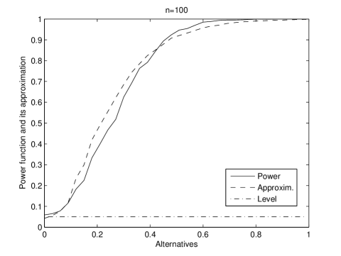
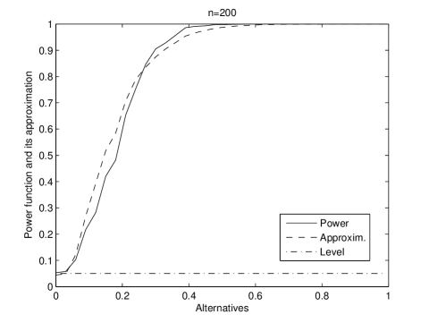
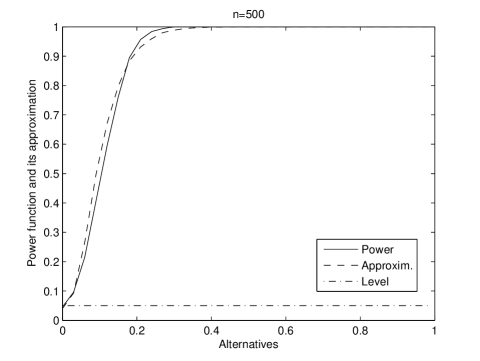
Figure 1. Approximation of the power function

7. Concluding remarks and possible developments

We have proposed new estimates and tests for model satisfying linear constraints with unknown parameter through divergence based methods which generalize the EL approach. This leads to the obtaining of the limiting distributions of the test statistics and the estimates under alternatives and under misspecification. Consistency of the test statistics under the alternatives is the starting point for the study of the optimality of the tests through Bahadur approach; also the generalized Neyman-Pearson optimality of EL test (as developed by Kitamura (2001)) can be adapted for empirical divergence based methods. Many problems remain to be studied in the future such as the choice of the divergence which leads to an optimal (in some sense) estimator or test in terms of efficiency and/or robustness. Preliminary simulation results show that Hellinger divergence enjoys good properties in terms of efficiency-robustness; see Broniatowski and Keziou (2008). Also comparisons under local alternatives should be developed.

8. Appendix

Proof of Theorem 5.1.
The same arguments, used for the proof of Theorem 3.1 in Newey and Smith (2004), hold when their criterion function $(\theta,\lambda)\in\Theta\times\mathbb{R}^{l}\mapsto\frac{1}{n}\sum_{i=1}^{n}\rho(\lambda^{\top}g(X,\theta))$ is replaced by our function $(\theta,t)\in\Theta\times\mathbb{R}^{1+l}\mapsto\frac{1}{n}\sum_{i=1}^{n}m(t^{\top}\overline{g}(X,\theta)).$ In particular, we have

$$\max_{1\leq i\leq n}\left|\widehat{t}(\widehat{\theta}_{\varphi})^{\top}\overline{g}(X_{i},\widehat{\theta}_{\varphi})\right|\to 0$$

in probability, which implies that $\widehat{t}(\widehat{\theta}_{\varphi})\in\text{int}(\Lambda^{(n)}_{\widehat{\theta}_{\varphi}})$ with probability one as $n\to\infty$, since $a^{*}<0<b^{*}$.

Proof of Theorem 5.2.
The proof is similar to that of Newey and Smith (2004) Theorem 3.2. Hence, it is omitted.

Proof of Theorem 5.3.
It is a particular case of Theorem 5.1 taking $\Theta=\{\theta\}.$ Hence, the proof is omitted.

Proof of Theorem 5.4.
1) First, note that $t^{*}(\theta)$ exists and is unique by Assumption 4. By the uniform weal law of large numbers (UWLLN), using continuity of $m(X,\theta,t)$ in $t$, and Assumption 4.b, we obtain

$$\left|P_{n}m(\theta,t)-\mathbb{E}\left[m(X,\theta,t)\right]\right|\to 0,$$ (8.1)

in probability uniformly in $t$ over the compact set $N_{t^{*}(\theta)}$. Using this and the fact that $t^{*}(\theta):=\arg\sup_{t\in\Lambda_{\theta}}P_{0}m(\theta,t)$ is unique and belongs to $\text{int}(N_{t^{*}(\theta)})$ and the strict concavity of $t\mapsto P_{0}m(\theta,t)$, we conclude that any value

$$\overline{t}:=\arg\sup_{t\in N_{t^{*}(\theta)}}P_{n}m(\theta,t)$$ (8.2)

converges in probability to $t^{*}(\theta)$; see e.g. Theorem 5.7 in van der Vaart (1998). We end then the proof by showing that $\widehat{t}(\theta)$ belongs to $\text{int}(N_{t^{*}(\theta)})$ with probability one as $n\to\infty$, and therefore it converges to $t^{*}(\theta).$ In fact, since for $n$ sufficiently large any value $\overline{t}$ lies in the interior of $N_{t^{*}(\theta)}$, concavity of $t\mapsto P_{n}m(\theta,t)$ implies that no other point $t$ in the complement of $\text{int}(N_{t^{*}(\theta)})$ can maximize $P_{n}m(\theta,t)$ over $t\in\mathbb{R}^{1+l}$, hence $\widehat{t}(\theta)$ must belongs to $\text{int}(N_{t^{*}(\theta)})$.
2) With probability tending to $1$ as $n\to\infty$, we have $\widehat{D}_{\varphi}(\mathcal{M}_{\theta},P_{0})=P_{n}m(\theta,\widehat{t})=P_{n}m(\theta,\overline{t})$. Hence, we can write

$$\left|\widehat{D}_{\varphi}(\mathcal{M}_{\theta},P_{0})-D_{\varphi}(\mathcal{M}_{\theta},P_{0})\right|=\left|P_{n}m(\theta,\overline{t})-P_{0}m(\theta,t^{*}(\theta))\right|=:|A|,$$

and

$$P_{n}m(\theta,t^{*}(\theta))-P_{0}m(\theta,t^{*}(\theta))\leq A\leq P_{n}m(\theta,\overline{t})-P_{0}m(\theta,\overline{t}).$$

Both the RHS and the LHS in the above display tend to $0$ in probability by (8.1). Hence, $\left|\widehat{D}_{\varphi}(\mathcal{M}_{\theta},P_{0})-D_{\varphi}(\mathcal{M}_{\theta},P_{0})\right|$ tends to $0$ in probability as $n\to\infty$. This ends the proof.

Proof of Theorem 5.5.
1) For $n$ sufficiently large, by a Taylor expansion, there exists $\overline{t}\in\mathbb{R}^{1+l}$ inside the segment that links $\widehat{t}$ and $t^{*}(\theta)$ with

$$\begin{array}[]{ccl}0&=&P_{n}m^{\prime}(\theta,\widehat{t})\\ &=&P_{n}m^{\prime}(\theta,t^{*}(\theta))+\left(P_{n}m^{\prime\prime}(\theta,\overline{t})\right)^{\top}\left(\widehat{t}-t^{*}(\theta)\right).\end{array}$$ (8.3)

By Assumptions 5.a and 5.b, using the fact that $\overline{t}=t^{*}(\theta)+o_{P}(1)$ and the UWLLN, we can prove that

$$P_{n}m^{\prime\prime}(\theta,\overline{t})=P_{0}m^{\prime\prime}(\theta,t^{*}(\theta))+o_{P}(1).$$

Using this display, one gets from (8.3)

$$-P_{n}m^{\prime}(\theta,t^{*}(\theta))=\left(P_{0}m^{\prime\prime}(\theta,t^{*}(\theta))+o_{P}(1)\right)\left(\widehat{t}-t^{*}(\theta)\right).$$ (8.4)

Assumptions 4.a and 5.a imply that $P_{0}m^{\prime}(\theta,t^{*}(\theta))=0$. Hence, by the central limit theorem (CLT), we have

$$\sqrt{n}P_{n}m^{\prime}(\theta,t^{*}(\theta))=O_{P}(1),$$

which by (8.4) implies that $\sqrt{n}\left(\widehat{t}-t^{*}(\theta)\right)=O_{P}(1).$ Hence, from (8.4), we get

$$\sqrt{n}\left(\widehat{t}-t^{*}(\theta)\right)={\left[-P_{0}m^{\prime\prime}(\theta,t^{*}(\theta))\right]}^{-1}\sqrt{n}P_{n}m^{\prime}(\theta,t^{*}(\theta))+o_{P}(1).$$ (8.5)

The CL and Slutsky theorems conclude the proof of part 1.
2) Using the fact that $\left(\widehat{t}-t^{*}(\theta)\right)=O_{P}(1/\sqrt{n})$ and $P_{n}m^{\prime}(\theta,t^{*}(\theta))=P_{0}m^{\prime}(\theta,t^{*}(\theta))+o_{P}(1)=0+o_{P}(1)=o_{P}(1)$, we obtain

$$\sqrt{n}\left(\widehat{D}_{\varphi}(\mathcal{M}_{\theta},P_{0})-D_{\varphi}(\mathcal{M}_{\theta},P_{0})\right) = \sqrt{n}\left(P_{n}m(\theta,\widehat{t})-P_{0}m(\theta,t^{*}(\theta))\right)$$

$$= \sqrt{n}\left(P_{n}m(\theta,t^{*}(\theta))-P_{0}m(\theta,t^{*}(\theta))\right)+o_{P}(1),$$

and the CL and Slutsky theorems conclude the proof.

Proof of Theorem 5.6.
1) First note that Assumption 6.d implies that the function $t\in\Lambda_{\theta}\mapsto\mathbb{E}m(X,\theta,t)$ is strictly concave for all $\theta\in\Theta$, which implies that $t^{*}(\theta)$ is unique for all $\theta\in\Theta$. By the UWLLN, using continuity of $m(X,\theta,t)$, in $\theta$ and $t$, and Assumption 6.c, we obtain the uniform convergence in probability, over the compact set $\left\{(\theta,t)\in\Theta\times\mathbb{R}^{1+l};~{}\theta\in\Theta,t\in N_{t^{*}(\theta)}\right\}$,

$$\sup_{\{\theta\in\Theta,t\in N_{t^{*}(\theta)}\}}\left|P_{n}m(\theta,t)-P_{0}m(\theta,t)\right|\to 0.$$ (8.6)

We can then prove the convergence in probability $\sup_{\theta\in\Theta}\|\widehat{t}(\theta)-t^{*}(\theta)\|\to 0$ in two steps. Step 1: Let $\eta>0$. We will show that $P_{0}\left[\sup_{\theta\in\Theta}\|\overline{t}(\theta)-t^{*}(\theta)\|\geq\eta\right]\to 0$ for any value

$$\overline{t}(\theta):=\arg\sup_{t\in N_{t^{*}(\theta)}}P_{n}m(\theta,t).$$ (8.7)

Step 2: To conclude the proof, we will show that $\widehat{t}(\theta)$ belongs to $\text{int}(N_{t^{*}(\theta)})$ with probability one as $n\to\infty$ for all $\theta\in\Theta$. Let $\eta>0$ such that $\sup_{\theta\in\Theta}\|\overline{t}(\theta)-t^{*}(\theta)\|\geq\eta$. Sine $\Theta$ is a compact set, by continuity there exists $\overline{\theta}\in\Theta$ such that $\sup_{\theta\in\Theta}\|\overline{t}(\theta)-t^{*}(\theta)\|=\|\overline{t}(\overline{\theta})-t^{*}(\overline{\theta})\|\geq\eta$. Hence, there exists $\varepsilon>0$ such that $P_{0}m(\overline{\theta},t^{*}(\overline{\theta}))-P_{0}m(\overline{\theta},\overline{t}(\overline{\theta}))>\varepsilon$. In fact, $\varepsilon$ may be defined as follows

$$\varepsilon:=\inf_{\theta\in\Theta}\sup_{\{t\in N_{t^{*}(\theta)};~{}\|t-t^{*}(\theta)\|\geq\eta\}}\mathbb{E}[m(X,\theta,t^{*}(\theta))]-\mathbb{E}[m(X,\theta,t)],$$

which is strictly positive by the strict concavity of $\mathbb{E}[m(X,\theta,t)]$ in $t$ for all $\theta\in\Theta$, the uniqueness of $t^{*}(\theta)\in\text{int}(N_{t^{*}(\theta)})$ and the fact that $\Theta$ is compact. Hence the event $\left[\sup_{\theta\in\Theta}\|\overline{t}(\theta)-t^{*}(\theta)\|\geq\eta\right]$ implies the event

$$\left[P_{0}m(\overline{\theta},t^{*}(\overline{\theta}))-P_{0}m(\overline{\theta},\overline{t}(\theta))\geq\varepsilon\right],$$

from which we obtain

$$P_{0}\left[\sup_{\theta\in\Theta}\|\overline{t}(\theta)-t^{*}(\theta)\|\geq\eta\right]\leq P_{0}\left[P_{0}m(\overline{\theta},t^{*}(\overline{\theta}))-P_{0}m(\overline{\theta},\overline{t}(\theta))\geq\varepsilon\right].$$ (8.8)

On the other hand, by (8.6), we have

$$P_{0}m(\overline{\theta},t^{*}(\overline{\theta}))-P_{0}m(\overline{\theta},\overline{t}(\theta)) = P_{n}m(\overline{\theta},t^{*}(\overline{\theta}))-P_{0}m(\overline{\theta},\overline{t}(\theta))+o_{P}(1)$$

$$\leq P_{n}m(\overline{\theta},\overline{t}(\overline{\theta}))-P_{0}m(\overline{\theta},\overline{t}(\theta))+o_{P}(1)$$

$$\leq \sup_{\{\theta\in\Theta,t\in N_{t^{*}(\theta)}\}}|P_{n}m(\theta,t)-P_{0}m(\theta,t)|+o_{P}(1).$$

Combining this with (8.8) and (8.6), we conclude that

$$\sup_{\theta\in\Theta}\|\overline{t}(\theta)-t^{*}(\theta)\|\to 0$$ (8.9)

in probability. In particular, $\overline{t}(\theta)\in\text{int}(N_{t^{*}(\theta)})$ for sufficiently large $n$, uniformly in $\theta\in\Theta$. Since $t\mapsto P_{n}m(\theta,t)$ is concave, then the maximizer $\widehat{t}(\theta)$ belongs to $\text{int}(N_{t^{*}(\theta)})$ for sufficiently large $n$; hence the same result (8.9) holds when $\overline{t}(\theta)$ is replaced by $\widehat{t}(\theta)$.
2) From part 1, we have for large $n$,

$$\sup_{\theta\in\Theta}|P_{n}m(\theta,\widehat{t}(\theta))-P_{0}m(\theta,t^{*}(\theta))| = \sup_{\theta\in\Theta}|P_{n}m(\theta,\overline{t}(\theta))-P_{0}m(\theta,t^{*}(\theta))|=:\sup_{\theta\in\Theta}|B|.$$

On the other hand, we have

$$P_{n}m(\theta,t^{*}(\theta))-P_{0}m(\theta,t^{*}(\theta))\leq B\leq P_{n}m(\theta,\overline{t}(\theta))-P_{0}m(\theta,\overline{t}(\theta)).$$

By Assumption 6.c, and the convergence in probability $\sup_{\theta\in\Theta}\|\overline{t}(\theta)-t^{*}(\theta)\|\to 0$, both the RHS and LHS of the above display tends to $0$ in probability uniformly in $\theta\in\Theta$, by the UWLLN. Hence, $\sup_{\theta\in\Theta}|P_{n}m(\theta,\widehat{t}(\theta))-P_{0}m(\theta,t^{*}(\theta))|\to 0$ in probability. Now, since the minimizer $\theta^{*}$ of $\theta\mapsto P_{0}m(\theta,t^{*}(\theta))$ over the compact set $\Theta$ is unique and interior point of $\Theta$, by continuity and the above uniform convergence, we conclude that $\widehat{\theta}_{\varphi}$ tends in probability to $\theta^{*}$; see e.g. Theorem 5.7 in van der Vaart (1998).
3) This holds as a consequence of the uniform convergence in probability

$$\sup_{\theta\in\Theta}|P_{n}m(\theta,\widehat{t}(\theta))-P_{0}m(\theta,t^{*}(\theta))|\to 0$$ (8.10)

proved in part 2 above. In fact, we have for $n$ sufficiently large

$$|\widehat{D}_{\varphi}(\mathcal{M},P_{0})-D_{\varphi}(\mathcal{M},P_{0})|=|P_{n}m(\widehat{\theta},\widehat{t}(\widehat{\theta}))-P_{0}m(\theta^{*},t^{*}(\theta^{*}))|=:|C|,$$

with

$$P_{n}m(\widehat{\theta},\widehat{t}(\widehat{\theta}))-P_{0}m(\widehat{\theta},t^{*}(\widehat{\theta}))\leq C\leq P_{n}m(\theta^{*},\widehat{t}(\theta^{*}))-P_{0}m(\theta^{*},t^{*}(\theta^{*}))$$

and both the RHS and LHS tend to $0$ in probability by (8.10). This concludes the proof.

Proof of Theorem 5.7.
1) By the first order conditions, with probability tending to one, we have

$$\left\{\begin{array}[]{lll}P_{n}\frac{\partial}{\partial t}m\left(\widehat{\theta},\widehat{t}(\widehat{\theta})\right)&=&0\\ P_{n}\frac{\partial}{\partial\theta}m\left(\widehat{\theta},\widehat{t}(\widehat{\theta})\right)+P_{n}\frac{\partial}{\partial t}m\left(\widehat{\theta},\widehat{t}(\widehat{\theta})\right)\frac{\partial}{\partial\theta}\widehat{t}(\widehat{\theta})&=&0.\end{array}\right.$$

The second term in the LHS of the second equation is equal to $0$, due to the first equation. Hence, $\widehat{t}(\widehat{\theta})$ and $\widehat{\theta}$ are solutions of the somehow simpler system

$$P_{n}\frac{\partial}{\partial t}m\left(\widehat{\theta},\widehat{t}(\widehat{\theta})\right) = 0$$ (8.11)

$$P_{n}\frac{\partial}{\partial\theta}m\left(\widehat{\theta},\widehat{t}(\widehat{\theta})\right) = 0.$$ (8.12)

Using a Taylor expansion in (8.11) in $(\widehat{\theta},\widehat{t})$ around $(\theta^{*},t^{*})$; there exists $\left(\overline{\theta},\overline{t}\right)$ inside the segment that links $(\widehat{\theta},\widehat{t}(\widehat{\theta}))$ and $(\theta^{*},t^{*}(\theta^{*}))$ such that

$$0 = P_{n}\frac{\partial}{\partial t}m\left(\theta^{*},t^{*}(\theta^{*})\right)+\left[\left(P_{n}\frac{\partial^{2}}{\partial t^{2}}m(\overline{\theta},\overline{c})\right)^{\top},\left(P_{n}\frac{\partial^{2}}{\partial\theta\partial t}m(\overline{\theta},\overline{c})\right)^{\top}\right]a_{n}$$

with

$$a_{n}:={\left({\left(\widehat{t}(\widehat{\theta})-t^{*}(\theta^{*})\right)}^{\top},{\left(\widehat{\theta}-\theta^{*}\right)}^{\top}\right)}^{\top}.$$ (8.14)

By Assumption 7, using the UWLLN, we can write

$$\left[P_{n}\frac{\partial^{2}}{\partial t^{2}}m(\overline{\theta},\overline{c}),P_{n}\frac{\partial^{2}}{\partial\theta\partial t}m(\overline{\theta},\overline{c})\right]=\left[P_{0}\frac{\partial^{2}}{\partial t^{2}}m(\theta^{*},t^{*}(\theta^{*})),P_{0}\frac{\partial^{2}}{\partial\theta\partial t}m(\theta^{*},t^{*}(\theta^{*}))\right]+o_{P}(1),$$

to obtain from (8)

$$-P_{n}\frac{\partial}{\partial t}m(\theta^{*},t^{*})=\left[\left(P_{0}\frac{\partial^{2}}{\partial t^{2}}m(\theta^{*},t^{*})\right)^{\top}+o_{P}(1),\left(P_{0}\frac{\partial^{2}}{\partial\theta\partial t}m(\theta^{*},t^{*})\right)^{\top}+o_{P}(1)\right]a_{n}.$$ (8.15)

In the same way, using a Taylor expansion in (8.12), we obtain

$$-P_{n}\frac{\partial}{\partial\theta}m(\theta^{*},t^{*})=\left[\left(P_{0}\frac{\partial^{2}}{\partial t\partial\theta}m(\theta^{*},t^{*})\right)^{\top}+o_{P}(1),\left(P_{0}\frac{\partial^{2}}{\partial\theta^{2}}m(\theta^{*},t^{*})\right)^{\top}+o_{P}(1)\right]a_{n}.$$ (8.16)

From (8.15) and (8.16), we get

$$\sqrt{n}a_{n} = \sqrt{n}\left(\begin{array}[]{cc}P_{0}\frac{\partial^{2}}{\partial t^{2}}m(\theta^{*},t^{*})&\left(P_{0}\frac{\partial^{2}}{\partial\theta\partial t}m(\theta^{*},t^{*})\right)^{\top}\\ \left(P_{0}\frac{\partial^{2}}{\partial t\partial\theta}m(\theta^{*},t^{*})\right)^{\top}&P_{0}\frac{\partial^{2}}{\partial\theta^{2}}m(\theta^{*},t^{*})\\ \end{array}\right)^{-1}\times$$ (8.22)

$$\times\left(\begin{array}[]{c}-P_{n}\frac{\partial}{\partial t}m(\theta^{*},t^{*})\\ -P_{n}\frac{\partial}{\partial\theta}m(\theta^{*},t^{*})\\ \end{array}\right)+o_{P}(1).$$

Denote $S$ the $(1+l+d)\times(1+l+d)-$matrix defined by

$$S:=\left(\begin{array}[]{cc}S_{11}&S_{12}\\ S_{21}&S_{22}\\ \end{array}\right):=\left(\begin{array}[]{cc}P_{0}\frac{\partial^{2}}{\partial t^{2}}m(\theta^{*},t^{*})&\left(P_{0}\frac{\partial^{2}}{\partial\theta\partial t}m(\theta^{*},t^{*})\right)^{\top}\\ \left(P_{0}\frac{\partial^{2}}{\partial t\partial\theta}m(\theta^{*},t^{*})\right)^{\top}&P_{0}\frac{\partial^{2}}{\partial\theta^{2}}m(\theta^{*},t^{*})\\ \end{array}\right).$$ (8.23)

Hence, we obtain

$$\sqrt{n}\left(\begin{array}[]{c}\widehat{t}(\widehat{\theta})-t^{*}(\theta^{*})\\ \widehat{\theta}-\theta^{*}\\ \end{array}\right)=\sqrt{n}S^{-1}\left(\begin{array}[]{c}-P_{n}\frac{\partial}{\partial t}m(\theta^{*},t^{*})\\ -P_{n}\frac{\partial}{\partial\theta}m(\theta^{*},t^{*})\\ \end{array}\right)+o_{P}(1),$$

and the CL and Slutsky theorems conclude the proof.
2) Using the fact that

$$\widehat{t}(\widehat{\theta})-t^{*}(\theta^{*})=O_{P}(1/\sqrt{n}),~{}P_{n}\partial m(\theta^{*},t^{*}(\theta^{*}))/\partial t=P_{0}\partial m(\theta^{*},t^{*}(\theta^{*}))/\partial t+o_{P}(1)=o_{P}(1)$$

and

$$\widehat{\theta}-\theta^{*}=O_{P}(1/\sqrt{n}),~{}P_{n}\partial m(\theta^{*},t^{*}(\theta^{*}))/\partial\theta=P_{0}\partial m(\theta^{*},t^{*}(\theta^{*}))/\partial\theta+o_{P}(1)=o_{P}(1),$$

we can write

$$\sqrt{n}\left(\widehat{D}_{\varphi}(\mathcal{M},P_{0})-D_{\varphi}(\mathcal{M},P_{0})\right) = \sqrt{n}\left(P_{n}m(\widehat{\theta},\widehat{t}(\widehat{\theta}))-P_{0}m(\theta^{*},t^{*}(\theta^{*}))\right)$$

$$= \sqrt{n}\left(P_{n}m(\theta^{*},t^{*}(\theta^{*}))-P_{0}m(\theta^{*},t^{*}(\theta^{*}))\right)+o_{P}(1),$$

and the CL and Slutsky theorems end the proof.

References

- Baggerly (1998) Baggerly, K. A. (1998). Empirical likelihood as a goodness-of-fit measure. Biometrika, 85(3), 535–547.
- Bertail (2006) Bertail, P. (2006). Empirical likelihood in some semiparametric models. Bernoulli, 12(2), 299–331.
- Broniatowski and Keziou (2006) Broniatowski, M. and Keziou, A. (2006). Minimization of -divergences on sets of signed measures. Studia Sci. Math. Hungar.; arXiv:1003.5457, 43(4), 403–442.
- Broniatowski and Keziou (2008) Broniatowski, M. and Keziou, A. (2008). Estimation and tests for models satisfying linear constraints with unknown parameter. arXiv:0811.3477v1.
- Broniatowski and Keziou (2009) Broniatowski, M. and Keziou, A. (2009). Parametric estimation and tests through divergences and the duality technique. J. Multivariate Anal., 100(1), 16–36.
- Chen et al. (2007) Chen, X., Hong, H., and Shum, M. (2007). Nonparametric likihood ratio model selection tests between parametric likelihood and moment condition models. J. Econometrics, 141(1), 109–140.
- Corcoran (1998) Corcoran, S. (1998). Bertlett adjustement of empirical discrepancy statistics. Biometrika, 85, 967–972.
- Cressie and Read (1984) Cressie, N. and Read, T. R. C. (1984). Multinomial goodness-of-fit tests. J. Roy. Statist. Soc. Ser. B, 46(3), 440–464.
- Csiszár (1963) Csiszár, I. (1963). Eine informationstheoretische Ungleichung und ihre Anwendung auf den Beweis der Ergodizität von Markoffschen Ketten. Magyar Tud. Akad. Mat. Kutató Int. Közl., 8, 85–108.
- Csiszár (1967) Csiszár, I. (1967). On topology properties of -divergences. Studia Sci. Math. Hungar., 2, 329–339.
- Haberman (1984) Haberman, S. J. (1984). Adjustment by minimum discriminant information. Ann. Statist., 12(3), 971–988.
- Hansen et al. (1996) Hansen, L., Heaton, J., and Yaron, A. (1996). Finite-sample properties of some alternative gmm estimators. Journal of Business and Economic Statistics, 14, 462–2800.
- Hansen (1982) Hansen, L. P. (1982). Large sample properties of generalized method of moments estimators. Econometrica, 50(4), 1029–1054.
- Hjort et al. (2009) Hjort, N. L., McKeague, I. W., and Van Keilegom, I. (2009). Extending the scope of empirical likelihood. Ann. Statist., 37(3), 1079–1111.
- Imbens (1997) Imbens, G. W. (1997). One-step estimators for over-identified generalized method of moments models. Rev. Econom. Stud., 64(3), 359–383.
- Keziou (2003) Keziou, A. (2003). Dual representation of -divergences and applications. C. R. Math. Acad. Sci. Paris, 336(10), 857–862.
- Kitamura (2001) Kitamura, Y. (2001). Asymptotic optimality of empirical likelihood for testing moment restrictions. Econometrica, 69(6), 1661–1672.
- Kitamura (2007) Kitamura, Y. (2007). Empirical likelihood methods in econometric theory and practice. Cambridge University Press.
- Liese and Vajda (1987) Liese, F. and Vajda, I. (1987). Convex statistical distances, volume 95. BSB B. G. Teubner Verlagsgesellschaft, Leipzig.
- McCullagh and Nelder (1983) McCullagh, P. and Nelder, J. A. (1983). Generalized linear models. Monographs on Statistics and Applied Probability. Chapman & Hall, London.
- Newey and Smith (2004) Newey, W. K. and Smith, R. J. (2004). Higher order properties of GMM and generalized empirical likelihood estimators. Econometrica, 72(1), 219–255.
- Owen (1990) Owen, A. (1990). Empirical likelihood ratio confidence regions. Ann. Statist., 18(1), 90–120.
- Owen (1991) Owen, A. (1991). Empirical likelihood for linear models. Ann. Statist., 19(4), 1725–1747.
- Owen (1988) Owen, A. B. (1988). Empirical likelihood ratio confidence intervals for a single functional. Biometrika, 75(2), 237–249.
- Owen (2001) Owen, A. B. (2001). Empirical Likelihood. Chapman and Hall, New York.
- Pardo (2006) Pardo, L. (2006). Statistical inference based on divergence measures, volume 185 of Statistics: Textbooks and Monographs. Chapman & Hall/CRC, Boca Raton, FL.
- Qin and Lawless (1994) Qin, J. and Lawless, J. (1994). Empirical likelihood and general estimating equations. Ann. Statist., 22(1), 300–325.
- Rockafellar (1970) Rockafellar, R. T. (1970). Convex analysis. Princeton University Press, Princeton, N.J.
- Schennach (2007) Schennach, S. M. (2007). Point estimation with exponentially tilted empirical likelihood. Ann. Statist., 35(2), 634–672.
- Sheehy (1987) Sheehy, A. (1987). Kullback-Leibler constrained estimation of probability measures. Report, Dept. Statistics, Stanford Univ.
- Smith (1997) Smith, R. J. (1997). Alternative semi-parametric likelihood approches to generalized method of moments estimation. Economic Journal, 107, 503–519.
- van der Vaart (1998) van der Vaart, A. W. (1998). Asymptotic statistics. Cambridge Series in Statistical and Probabilistic Mathematics. Cambridge University Press, Cambridge.
- White (1982) White, H. (1982). Maximum likelihood estimation of misspecified models. Econometrica, 50(1), 1–25.