Buckling of Graphene Layers Supported by Rigid Substrates

Abstract

We formulate a nonlinear continuum model of a graphene sheet supported by a flat rigid substrate. The sheet is parallel to the substrate and loaded on a pair of opposite edges. A typical cross-section of the sheet is modeled as an elastica. We use elementary techniques from bifurcation theory to investigate how the buckling of the sheet depends on the boundary conditions, the composition of the substrate, and the length of the sheet. We also present numerical results that illustrate snap-buckling of the sheet.

Keywords: graphene, mechanical behavior, van der Waals forces, elastica, elastic foundation

1 Introduction

A graphene sheet is a planar hexagonal lattice of carbon atoms with each atom bonded to its three nearest neighbors. Theoretical predictions about the properties of graphene as well as the role graphene plays as the basic structure in other important materials, in particular bulk graphite and carbon nanotubes, have driven efforts to produce isolated single-layer graphene sheets. Somewhat surprisingly, these efforts succeeded only recently, with the discovery of mechanical and chemical methods for isolating individual graphene sheets and functionalized sheets from bulk graphite [23, 24, 36]. The last several years have brought a tremendous amount of theoretical and experimental research on graphene.

Much of this recent research explores the novel electronic transport properties of graphene. To a lesser extent, the mechanical properties of graphene have also attracted attention. Transport properties suggest engineering nanoscale devices that use graphene as basic components like nanoscale resonators, switches, and valves. See, for example, [3]. Mechanical properties suggest the use of graphene in composite materials [27, 39]. For the latter, understanding the response of individual graphene sheets to applied loads is clearly important. Additionally, for designing graphene-based devices, and more generally for exploiting the transport properties of graphene, an understanding of the mechanical response of graphene may prove essential for at least two reasons. First, to assemble nanoscale components, it may be useful to develop techniques for manipulating individual graphene sheets and related nanoscale structures, which entails understanding how these sheets respond to applied loads [18, 29, 47]. Second, research suggests that the electronic transport properties of graphene are coupled to its mechanical deformation [4, 7, 12, 13, 21, 33].

In this paper we study the mechanical response of a graphene sheet parallel to and supported by a flat rigid substrate. The sheet is loaded compressively on a pair of opposite edges. See Figure 1 below. The problem we formulate can be loosely motivated by a recent experimental paper of Schniepp et al. [35], in which functionalized graphene sheets supported on a substrate of highly oriented pyrolytic graphite (HOPG) are manipulated with the tip of an atomic force microscope (AFM). The authors show that the lateral force exerted on the edge of the sheet by the AFM tip can slide the sheet across the substrate or, more interestingly, can fold the edge of the sheet. See Figures 3 and 4 in [35]. In fact, the sheet can be folded and unfolded by the tip multiple times with this repeated folding occurring along the same location. In our idealized continuum model, the compressive load on the edges of the sheet could describe the lateral load applied by an AFM tip. More generally, the geometry of our problem seems fundamental for the study of the mechanics of graphene because mechanical exfoliation, a technique for isolating individual graphene from bulk graphite, yields graphene sheets supported by a rigid substrate [24]. Also, several proposed electronic devices are based on graphene in a geometry similar to that of our problem [33].

We consider two types of substrates. In one case, the sheet interacts with SiO₂, a material commonly used to isolate single-layer graphene by mechanical exfoliation [2]. The interaction between the flexible sheet and the substrate is by van der Waals forces, which act over a short-range between the individual carbon atoms on the sheet and the atoms in the substrate. Several recent papers suggest that the mechanical response of graphene supported on SiO₂ is significantly influenced by the interaction between the sheet and the substrate [33]. As a second case, we consider a graphene sheet interacting by van der Waals forces with a second, rigid graphene sheet. The interaction between two graphene sheets should approximate well the interaction between graphene and the HOPG substrate in the experiments in [35] (although we note that the specific interaction terms we present in the next section are appropriate for describing a substrate supporting pure graphene, not functionalized graphene).

Modeling both the graphene sheet and the substrate as continua, we derive equilibrium equations for the static response of the compressively loaded sheet. We assume that the sheet deforms the same in each cross-section, a simplification supported by the atomistic simulations in [17, 45]. A typical cross-section of the sheet is modeled as an elastic rod. Our assumptions along with appropriate boundary conditions—discussed in the next paragraph— yield a geometrically exact version of the classical problem of a beam on a nonlinearly elastic foundation.

Two sets of boundary conditions are considered. For the first set, the horizontal component of the applied load at opposite edges of the sheet is prescribed, the loaded edges are moment free, and the loaded edges are kept at a prescribed distance from the substrate. These correspond to classical ‘hinged’ boundary conditions. For the second set of boundary conditions, we again prescribe the horizontal component of the applied load at opposite edges and we require that the loaded edges are moment free. But the loaded edges are not kept a prescribed distance from the substrate. Rather, the vertical component of the applied load is prescribed to be zero. This second set of conditions is loosely motivated by the AFM tip experiments described above, in which the edges of the sheet folded over as the lateral load was applied.

Using standard ideas from bifurcation theory, we investigate how the mechanical response of the graphene sheet depends on the length of the sheet, on the boundary conditions, and on the composition of the substrate. In our bifurcation analysis, the trivial branch corresponds to a flat sheet parallel to and at the equilibrium spacing from the substrate. By linearizing about the trivial branch, we compute the critical load at which the sheet buckles. How this critical load depends on length, boundary conditions, and the composition of the substrate is summarized in Table 1. We show that the critical load converges to a nonzero value as the length of the sheet goes to infinity. To illuminate the post-buckling behavior, we numerically continue the branching solutions. Our numerical results indicate that the post-buckling behavior includes secondary bifurcations, and, more interestingly, snap-buckling.

There is an extensive literature on the buckling of single-walled and multi-walled carbon nanotubes under axial and radial loads. For results that use continuum modeling, see, for example, [30, 31, 37]. The literature on buckling of graphene sheets under compressive loading is less extensive. In [45], we studied the buckling under edge loads of two parallel, deformable graphene sheets interacting by van der Waals forces. We showed that a simple continuum model of buckling yields predictions that are qualitatively similar to the predictions of atomistic simulations. In [17], the authors studied the buckling of graphene nanoribbons under compressive load. The atomistic simulations they performed were based on energy minimization techniques in which the carbon-carbon interactions were modeled by the REBO potential. Their results suggest that linear beam theory predicts reasonably well the buckling of graphene. In their problem, the sheet did not interact with a substrate. In [34], the author used the ‘molecular structural mechanics’ approach developed in [15] to perform atomistic simulations of the buckling of a graphene sheet under compressive loading. How the boundary conditions, the length of the sheet, and the aspect ratio of the sheet influenced the buckling load were studied. In their model, the sheet is freely suspended and not interacting with a substrate. A comparison between Figures 2 and 3 and between Figures 4 and 5 in [34] suggests that for sheets with lateral dimensions larger than 25 nm, chirality does not strongly influence the buckling load. That the buckling load does not appear to depend on chirality was also noted in [17]. In our continuum model, we cannot describe the chirality of the sheet. In [26], the authors apply nonlocal elasticity theory to study the buckling of graphene sheets under biaxial compression. They study a single graphene sheet that is freely suspended and not interacting with a substrate. Figure 5 in [26] suggests that as the lateral dimensions of the sheet exceed about 25 nm nonlocal effects become less important for determining buckling loads. This observation supports the validity of our results, where nonlocal effects are not considered. We note also the recent paper [16], in which the authors study the morphology of a graphene sheet supported by a patterned substrate. Their results indicate that as a certain parameter controlling the pattern on the substrate is varied, the sheet can exhibit a ‘snap-through’ instability, which appears similar to the snap-buckling we describe below.

An interesting issue related to the basic morphology of a graphene sheet supported on a substrate is the existence of ripples [19]. Several theories have been proposed to explain this rippling [4, 6, 9, 11, 42]. Here we do not directly address the question of rippling.

In the next section, we derive the boundary-value-problem for a graphene sheet interacting with a substrate. In Section 3, we identify a trivial branch and compute buckling loads. Section 4 contains numerical results that describe post-buckling behavior. The final section summarizes our results and mentions several additional problems that could be studied within the framework of the model we develop.

2 Equilibrium Equations

To describe the basic geometry of our problem, we let $\{\mathbf{i},\mathbf{j},\mathbf{k}\}$ denote a right-handed orthonormal basis for $\mathbb{R}^{3}$. The rigid substrate is parallel to the $\mathbf{i}\mathbf{k}$-plane, and $\mathbf{j}$ points away from the substrate. See Figure 1. We assume the deformation of the sheet is the same in any cross-section defined by a plane perpendicular to $\mathbf{k}$, and hence the configuration of the sheet is determined by the configuration of a typical cross-section. A cross-section is described by a curve $[0,L]\ni s\mapsto\mathbf{r}(s)$ in the $\mathbf{i}\mathbf{j}$-plane.

Figure 1: Basic geometry of a typical cross-section.

For the geometry depicted in Figure 1, an appropriate theory of nonlinear rods (see [1]) delivers the governing equations

(2.1) $$\mathbf{n}^{\prime}+\mathbf{f}=\mathbf{0},\qquad M^{\prime}+\mathbf{k}\cdot(\mathbf{r}^{\prime}\times\mathbf{n})=0,$$

(2.2) $$\mathbf{n}(0)\cdot\mathbf{i}=\mathbf{n}(L)\cdot\mathbf{i}=-\nu,\qquad M(0)=M(L)=0,$$

which are the linear and angular momentum balances for the sheet supplemented by boundary conditions. In (2.1), (2.2), $\mathbf{n}(s)$ is the contact force per unit width on the material point $s$, $\mathbf{f}(s)$ is the force per unit area exerted by the substrate on $s$, and $M(s)$ is the $\mathbf{k}$ component of the contact torque per unit width on $s$. The boundary condition $\eqref{c1}\raisebox{-2.84526pt}{\scriptsize 1}$ describes the load applied to opposite edges of the sheet. The parameter $\nu$ is the component of the load parallel to the substrate at the left edge; $\nu>0$ corresponds to compressive loading. The boundary condition $\eqref{c1}\raisebox{-2.84526pt}{\scriptsize 2}$ states that the loaded edges are moment free. Additional boundary conditions are given below.

To introduce components, we write

(2.3) $$\mathbf{r}(s)=x(s)\mathbf{i}+(y(s)+\bar{d})\mathbf{j},\qquad\mathbf{n}(s)=P(s)\mathbf{i}+Q(s)\mathbf{j},$$

where the constant $\bar{d}$ is defined later. We assume the cross-section of the layer is inextensible, so that

(2.4) $$\mathbf{r}^{\prime}(s)=x^{\prime}(s)\mathbf{i}+y^{\prime}(s)\mathbf{j}=\cos\theta(s)\mathbf{i}+\sin\theta(s)\mathbf{j}$$

for some function $[0,L]\ni s\mapsto\theta(s)$. Hence $L$ is the length of the sheet. We also assume that $M(s)=\alpha\,\theta^{\prime}\!(s)$ for some constant $\alpha>0$, which is a material parameter describing the resistance of the sheet to bending. Values from the literature on the continuum modeling of graphene and carbon nanotubes suggest that one can choose $\alpha$ in a range between $.13$ and $.2$ nN nm [12, 14, 22, 28, 33, 41, 44, 46]. To make explicit computations below, we take $\alpha=0.16$ nN nm. Note that inextensibility and a linear dependence of the moment on the curvature are the standard assumptions of the elastica theory.

The term $\mathbf{f}$ in $\eqref{c4}\raisebox{-2.84526pt}{\scriptsize 1}$ describes the interaction force exerted by the substrate on the sheet. The specific form of $f$ depends on the composition of the substrate. One case we study is a substrate composed of SiO₂. To determine the interaction force in this case, we start with an expression for the attractive energy between graphene and SiO₂ from [33]. The authors report an attractive energy per unit area of

(2.5) $$E=-\frac{\hbar v_{F}}{4a}\frac{g_{1}+g_{2}}{\xi^{2}},$$

where $g_{1}=5.4\cdot 10^{-3}$, $g_{2}=3.5\cdot 10^{-2}$, $v_{F}=10^{6}$ m/s, $a=.142$ nm , $\hbar$ is Planck’s constant, and $\xi$ is the distance between the graphene sheet and the substrate. From (2.5), we derive an attractive force of the form $-c_{A}/\xi^{3}$, where $c_{A}=1.499\cdot 10^{-2}$ nN nm. Now we define $\mathbf{f}(s)=\bar{f}_{I}(y(s)+\bar{d}_{I})\mathbf{j}$, where $\bar{f}_{I}$ has the form

(2.6) $$\bar{f}_{I}(\xi)=\frac{c_{R}}{\xi^{11}}-\frac{c_{A}}{\xi^{3}}$$

with $c_{R}=1.499\cdot 10^{-2}$ nN nm⁹. The repulsive term in (2.6) is derived by first assuming a $\xi^{-11}$ dependence, which is consistent with the repulsive part of the Lennard-Jones potential used to describe the interaction between non-bonded atoms (see (2.7) below), and then choosing $c_{R}$ so that the equilibrium spacing between the sheet and the substrate is $\bar{d}_{I}=1$ nm, which is consistent with some experimental data [8, 40]. The graph of $\bar{f}_{I}$ is depicted in Figure 2(a).

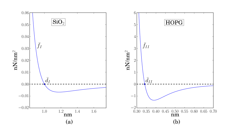
Figure 2: Interaction forces for (a) SiO₂ and (b) HOPG substrates. $\bar{d}_{I}=1$ nm and $\bar{d}_{II}=.341$ nm are the unique zeros of $\bar{f}_{I}$ and $\bar{f}_{II}$.

We also consider the case in which the substrate is HOPG. The force described by $\mathbf{f}$ in $\eqref{c4}\raisebox{-2.84526pt}{\scriptsize 1}$ arises because of van der Waals interactions between the carbon atoms of the sheet and the carbon atoms of the substrate. We consider the interactions between the sheet and only the top layer of the atoms on the HOPG substrate. Hence we model the substrate as a second, rigid sheet of graphene. (Because the van der Waals force between carbon atoms decays rapidly as the spacing between the atoms increases, including interactions with additional layers of the HOPG substrate does not significantly change the interaction force between the sheet and the substrate.) To define $\mathbf{f}$ appropriately for a continuum model, we assume the atoms are distributed on the substrate and on the sheet with a uniform atomic density $\sigma=38.177\ \mathrm{nm}^{-2}$, a value computed from the geometry of graphene. Also, we assume the substrate is infinite in extent. By computing an appropriate improper integral, we find that the force per unit area exerted by the substrate on the sheet is $\mathbf{f}(s)=\bar{f}_{II}(y(s)+\bar{d}_{II})\mathbf{j}$, where

(2.7) $$\bar{f}_{II}(\xi)=2\pi\sigma^{2}\left(\frac{c_{12}}{\xi^{11}}-\frac{c_{6}}{\xi^{5}}\right)$$

with $c_{12}=3.859\times 10^{-9}\ \mathrm{nN}\ \mathrm{nm}^{13}$ and $c_{6}=2.43\times 10^{-6}\ \mathrm{nN}\ \mathrm{nm}^{7}$. (See [45] for details. The values of $c_{6}$ and $c_{12}$ are from [10].) The graph of $\bar{f}_{II}$ is depicted in Figure 2(b). Note that $\bar{f}_{II}$ has a unique zero at $\bar{d}_{II}=(c_{12}/c_{6})^{1/6}=0.341$ nm, which is the equilibrium spacing.

Below we denote the $\mathbf{j}$ component of the interaction force by just $\bar{f}$ and indicate whether $\bar{f}=\bar{f}_{I}$ or $\bar{f}=\bar{f}_{II}$ only when presenting numerical results. We treat $\bar{d}$ likewise. Recalling $\eqref{c2}\raisebox{-2.84526pt}{\scriptsize 1}$, we see that the $\mathbf{j}$ component of $\mathbf{r}$ is measured from $\bar{d}$, so that $y(s)=0$ implies that $\mathbf{f}(s)=\mathbf{0}$.

We now reformulate (2.1), (2.2) in components. First we note that $$\mathbf{f}\cdot\mathbf{i}=0 \eqref{c4}\raisebox{-2.84526pt}{\scriptsize 1} \eqref{c2}\raisebox{-2.84526pt}{\scriptsize 2} P^{\prime}(s)=0 s P\equiv-\nu \eqref{c1}\raisebox{-2.84526pt}{\scriptsize 1}$$, , and imply that for all , and hence by . Then (2.1), (2.3), and (2.4) yield the system

(2.8a) $$y^{\prime} =\sin\theta,$$

(2.8b) $$M^{\prime} =-\nu\sin\theta-Q\cos\theta,$$

(2.8c) $$\theta^{\prime} =\alpha^{-1}M,$$

(2.8d) $$Q^{\prime} =-\bar{f}(y+\bar{d}).$$

We study this system with the boundary conditions

(2.8e) $$M(0)=M(L)=0,$$

which is $$\eqref{c1}\raisebox{-2.84526pt}{\scriptsize 2}$$, supplemented with either

(2.8f) $$y(0)=y(L)=0\qquad\text{or}\qquad Q(0)=Q(L)=0.$$

For conditions (2.8e), $\eqref{c9}\raisebox{-2.84526pt}{\scriptsize 1}$, the loaded edges are moment free and kept at a prescribed distance from the substrate. These conditions correspond to standard hinged boundary conditions. For conditions (2.8e), $\eqref{c9}\raisebox{-2.84526pt}{\scriptsize 2}$, the edge is moment free but not kept a prescribed distance from the substrate. Rather, the vertical component of the applied load is prescribed to be zero. Below we shall refer to this second set of conditions as the ‘floating-edge’ boundary conditions. (For boundary conditions $\eqref{c9}\raisebox{-2.84526pt}{\scriptsize 1}$, the applied load at the edge may have a non-zero vertical component.)

To non-dimensionalize, we define

(2.9) $$\hat{s}=\frac{s}{L},\quad\hat{y}(\hat{s})=\frac{y(s)}{L},\quad\hat{M}(\hat{s})=\frac{LM(s)}{\alpha},\quad\hat{\theta}(\hat{s})=\theta(s),$$

(2.10) $$\hat{Q}(\hat{s})=\frac{L^{2}}{\alpha}Q(s),\quad\hat{\nu}=\frac{L^{2}}{\alpha}\nu,\quad\hat{f}(\xi)=\frac{L^{3}}{\alpha}\bar{f}(L\xi+\bar{d}).$$

Upon inserting these rescalings into (2.8) (and dropping the hats), we get

(2.11a) $$y^{\prime} =\sin\theta,$$

(2.11b) $$M^{\prime} =-\nu\sin\theta-Q\cos\theta,$$

(2.11c) $$\theta^{\prime} =M,$$

(2.11d) $$Q^{\prime} =-f(y),$$

with boundary conditions

(2.12a) $$M(0)=M(1)=0,\quad\text{and}$$

(2.12b) $$y(0)=y(1)=0\quad\text{\ or}\quad Q(0)=Q(1)=0.$$

Note that the problem we have formulated is a version of the classical problem of a beam on an elastic foundation [43]. Our version differs from most treatments because we do not use the Euler-Bernoulli beam equation. Also, our choice for $\bar{f}$, which describes the interaction of the beam with the foundation, is specific to graphene supported by either an SiO₂ or HOPG substrate.

3 Buckling Loads

One checks that $(y,M,\theta,Q)=(0,0,0,0)$ is a solution to (2.11), (2.12) for all loads $\nu$. This solution corresponds to a flat sheet parallel to the substrate at the equilibrium spacing $\bar{d}$. In this section, we find the loads at which the sheet buckles from the flat configuration and we describe how these buckling loads depend on various parameters in the problem.

Linearizing (2.11) about the trivial branch yields

(3.1a) $$y^{\prime} =\theta,$$

(3.1b) $$M^{\prime} =-\nu\theta-Q,$$

(3.1c) $$\theta^{\prime} =M,$$

(3.1d) $$Q^{\prime} =-f_{1}y,$$

where $f_{1}:=f^{\prime}(0)=(L^{4}/\alpha)\bar{f}^{\prime}(\bar{d})$ by $\eqref{c26}\raisebox{-2.84526pt}{\scriptsize 3}$. From (2.6), (2.7), we have that $\bar{f}^{\prime}(\bar{d})=-.12$ nN/nm³ for $\bar{f}=\bar{f}_{I}$ and that $\bar{f}^{\prime}(\bar{d})=-84.1$ nN/nm³ for $\bar{f}=\bar{f}_{II}$. The linearized boundary conditions for (3.1) are the same as (2.12).

To locate critical loads, it is convenient though not essential to reformulate (3.1) as a single fourth-order equation. We do so by noting that

(3.2) $$\theta^{\prime\prime\prime\prime}=M^{\prime\prime\prime}=-\nu\theta^{\prime\prime}-Q^{\prime\prime}=-\nu\theta^{\prime\prime}+f_{1}y^{\prime}=-\nu\theta^{\prime\prime}+f_{1}\theta,$$

and hence

(3.3) $$\theta^{\prime\prime\prime\prime}+\nu\theta^{\prime\prime}-f_{1}\theta=0.$$

By (3.1c), the condition (2.12a) corresponds to $\theta^{\prime}(0)=\theta^{\prime}(1)=0$. Also, by (3.1b) and (3.1c), $Q=-\nu\theta-\theta^{\prime\prime}$, and then by (3.1d) $f_{1}y=\nu\theta^{\prime}+\theta^{\prime\prime\prime}$. Hence (2.12) implies that

(3.4a) $$\theta^{\prime}(0)=\theta^{\prime}(1)=0,\text{\ and}$$

(3.4b) $$\theta^{\prime\prime\prime}(0)=\theta^{\prime\prime\prime}(1)=0\quad\text{or}\quad\theta^{\prime\prime}(0)+\nu\theta(0)=\theta^{\prime\prime}(1)+\nu\theta(1)=0$$

are the two sets of boundary conditions for (3.3).

The critical loads are the values of $\nu$ at which (3.3), (3.4) has a non-trivial solution. For a given $\nu$, (3.3), (3.4) has a non-trivial solution if and only if (3.1), (2.12) has a non-trivial solution. To find non-trivial solutions of (3.3), (3.4), we compute the characteristic roots of (3.3), which are $\pm\sqrt{(-\nu\pm\sqrt{\nu^{2}+4f_{1}})/2}$. Using these roots, we find the general solution to (3.3), to which we apply one set of boundary conditions from (3.4). This yields a system of linear equations $M(\nu)\mathbf{c}=\mathbf{0}$ for the vector $\mathbf{c}\in\mathbb{R}^{4}$ of arbitrary constants in the general solution. Here $M(\nu)$ is a $4\times 4$ matrix whose entries depend nonlinearly on $\nu$. The buckling loads are the values of $\nu$ such that $M(\nu)\mathbf{c}=\mathbf{0}$ has non-trivial solutions. Hence it is sufficient to consider $\nu\mapsto\operatorname{det}(M(\nu))$. Performing the computations just described yields

(3.5) $$\operatorname{det}(M(\nu))=\sin\lambda_{1}\sin\lambda_{2}$$

for the boundary conditions (3.4a), $\eqref{c54}\raisebox{-2.84526pt}{\scriptsize 1}$ and

(3.6) $$\operatorname{det}(M(\nu))=\sqrt{-f_{1}}\lambda_{2}\Biggl{(}2(\cos\lambda_{1}\cos\lambda_{2}-1)+\frac{\lambda_{1}^{6}+\lambda_{2}^{6}}{(-f_{1})^{3/2}}\sin\lambda_{1}\sin\lambda_{2}\Biggr{)}$$

for the boundary conditions (3.4a), $\eqref{c54}\raisebox{-2.84526pt}{\scriptsize 2}$, where

(3.7) $$\lambda_{1}=\sqrt{(\nu-\sqrt{\nu^{2}+4f_{1}})/2},\qquad\lambda_{2}=\sqrt{(\nu+\sqrt{\nu^{2}+4f_{1}})/2}.$$

The expressions (3.5) and (3.6) are correct for $\nu>2\sqrt{-f_{1}}$. One can show that there are no non-trivial solutions for $0<\nu\leq 2\sqrt{-f_{1}}$. Note that $f_{1}$ and hence $\operatorname{det}(M(\nu))$ depend on $\alpha$ and $L$. Also, note that (3.5) implies that either $\lambda_{1}=m\pi$ or $\lambda_{2}=m\pi$, which is equivalent to

(3.8) $$\nu=\pi^{2}m^{2}-f_{1}/\pi^{2}m^{2},$$

a formula that could be found more directly by substituting $\theta=A\cos(m\pi s)$ into (3.3), where $A$ is an arbitrary amplitude.

For a given length $L$, we let $\nu^{*}$ denote the buckling load, i.e., the smallest critical load. In the rest of this section, we illustrate how $\nu^{*}$ depends on the interaction force, the boundary conditions, the length of the sheet $L$, and the bending stiffness $\alpha$. These results are computed using either (3.5) or (3.6). For all the results described below, we take $\alpha=.16$ nN nm unless otherwise noted.

Figure 3 indicates how $\nu^{*}$ depends on the length $L$ of the sheet for graphene supported by an SiO₂ substrate. Figure 3 is for hinged boundary conditions (2.12a), $\eqref{c51}\raisebox{-2.84526pt}{\scriptsize 1}$. From the figure we see that as $L$ increases the buckling load oscillates. The local minima of these oscillations equal $.277$ nN/nm, the local maxima decrease, and $\nu^{*}$ converges to the value of the local minima as $L$ gets large. See also Figure 9 (a) below. This oscillatory behavior is well-known. See [38]. It occurs because the deformation mode of the buckled solutions changes at the cusps in Figures 3 (a), (b). In particular, across the cusps, the nodal behavior and the number of half-sine waves in the deformation mode change (see Figure 4, which is described in the next paragraph). Each deformation mode has a different critical load, and which mode has the lowest critical load changes at the cusps.

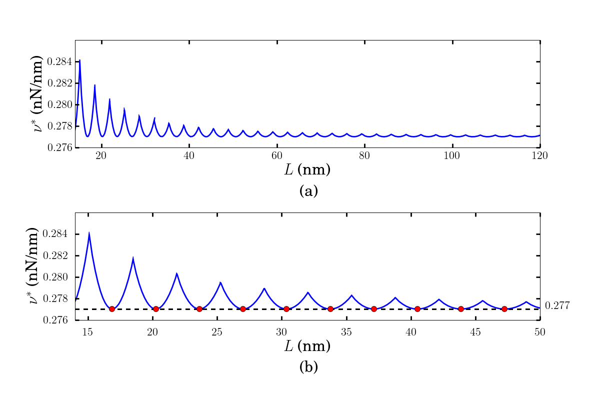
Figure 3: Buckling loads for SiO₂ substrate and hinged boundary conditions. Figures (a) and (b) show how the buckling load, denoted by $\nu^{*}$, depends on $L$ for $\alpha=.16$ nN nm.

Figure 4 illustrates how the nodal behavior of the buckled solutions changes at the values of $L$ that correspond to the cusps in Figures 3 (a), (b). For the curve describing $\nu^{*}$ as a function of $L$, there are cusps at $L=4.8$, $8.3$, $11.7$, and $15$. The second and third of these cusps can be seen in Figure 4 (a). Figure 4 (b) shows the buckled configuration corresponding to the buckling load $\nu^{*}$ for $L=6$ nm. The curve in Figure 4 (b) has a single simple zero, or node, on $(0,L)$, which is the case for all buckled solutions corresponding to lengths $L$ between $4.8$ and $8.3$. Figures 4 (c) and (d) show how the number of nodes of the buckled solutions increases for solutions corresponding to $L$ between $8.3$ and $11.7$ and for solutions corresponding to $L$ between $11.7$ and $15$.

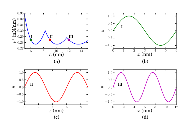
Figure 4: Shape of buckled solutions. Figure (a) shows how the buckling load $\nu^{*}$ depends on $L$ for $\alpha=.16$ nN nm and for graphene supported on an SiO₂ substrate with hinged boundary conditions. The points marked I, II, and III correspond to the buckling loads for $L=6$, $9$, and $12$ nm. Figures (b), (c), and (d) show how the nodal behavior of the corresponding buckled solutions changes across the two cusps located between the points labeled I, II, and III in (a). For each solution in (b), (c), and (d), the amplitude has been normalized to 1.

Figure 5 indicates how $\nu^{*}$ depends on $L$ for graphene supported by an SiO₂ substrate and loaded by the floating-edge boundary conditions (2.12a), $\eqref{c51}\raisebox{-2.84526pt}{\scriptsize 2}$. As in Figure 3, we see that as $L$ increases the buckling load oscillates. In this case, however, both the local minima and local maxima decrease as $L$ increases. Figure 5 (a) suggests that $\nu^{*}$ converges to a limiting value as $L$ gets large. See also Figure 9 (a) below. The behavior of the buckled solutions across the cusps is similar to that illustrated in Figure 4.

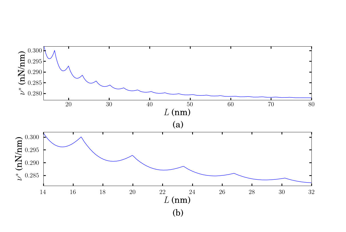
Figure 5: Buckling loads for graphene supported by an SiO₂ substrate with floating-edge boundary conditions. Figures (a) and (b) show how the buckling load $\nu^{*}$ depends on $L$ for $\alpha=.16$ nN nm.

Figures 6 and 7 illustrate how $\nu^{*}$ depends on $L$ for graphene supported by a HOPG substrate. Figure 6 is for hinged boundary conditions and Figure 7 is for floating-edge boundary conditions. Although both Figures 6 and Figure 7 are qualitatively similar to Figures 3 and Figure 5, which are the corresponding figures for graphene on SiO₂, we note that the predicted buckling loads the HOPG substrate are approximately an order of magnitude larger than the buckling loads for graphene supported by an SiO₂ substrate. For example, in Figure 3 (b), $\nu^{*}=0.2771$ nN/nm for $L=40$ nm while in Figure 6 (a), $\nu^{*}=7.335$ nN/nm for $L=40$ nm. See also Table 1. The difference in the size of the buckling loads predicted by the model is a consequence of the difference between the derivatives of the interaction forces at the equilibrium spacings— $\bar{f}^{\prime}_{I}(\bar{d}_{I})=-.12$ nN/nm³ for SiO₂ and $\bar{f}^{\prime}_{II}(\bar{d_{II}})=-84.1$ nN/nm³ for HOPG. Figure 8 illustrates how $\nu^{*}$ depends on $\bar{f}^{\prime}(\bar{d})$ for $L=5$ nm. Note that $-\bar{f}^{\prime}(\bar{d})$ represents the linear stiffness or ‘spring constant’ of the elastic foundation.

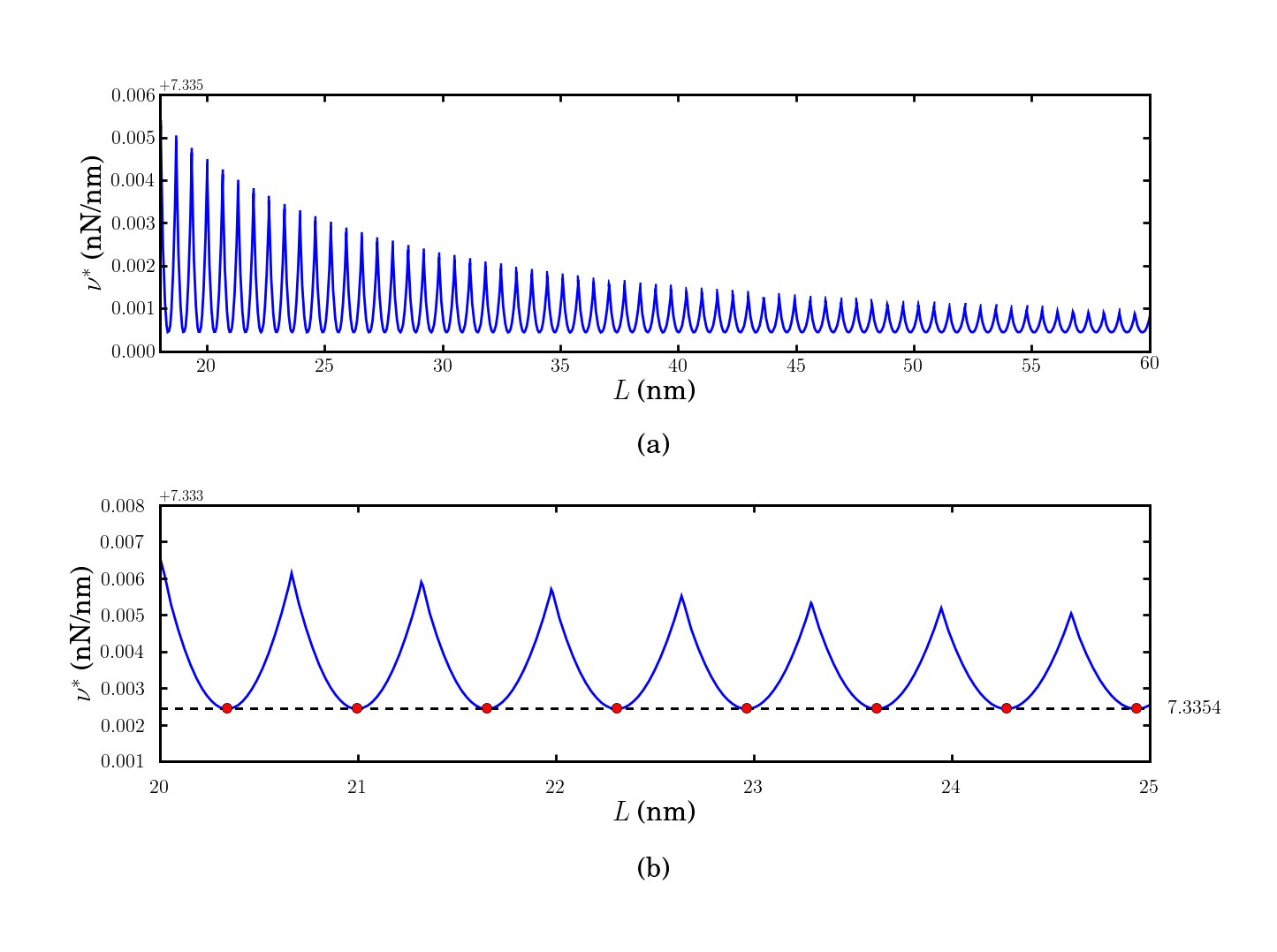
Figure 6: Buckling loads for HOPG substrate with hinged boundary conditions. Figures (a) and (b) show how the smallest eigenvalue, denoted by $\nu^{*}$, depends on $L$ for $\alpha=.16$ nN nm.

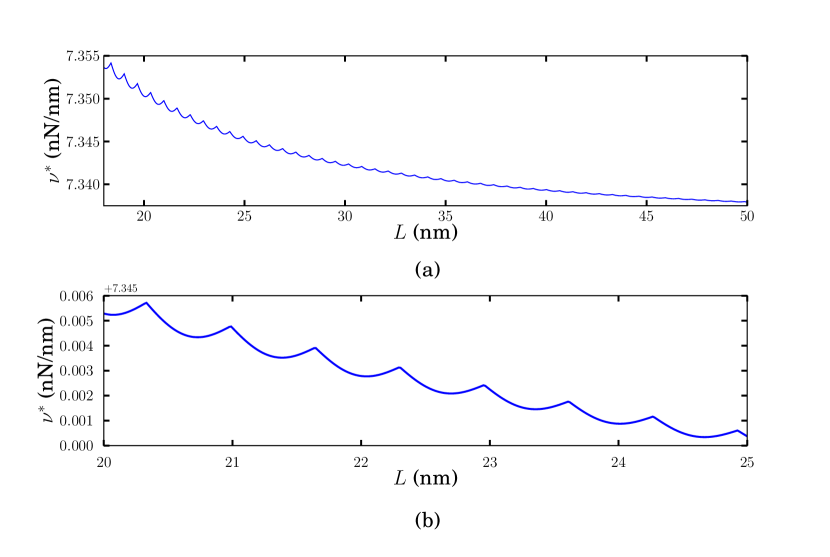
Figure 7: Buckling loads for HOPG substrate with floating-edge boundary conditions. Figures (a) and (b) show how the smallest eigenvalue, denoted by $\nu^{*}$, depends on $L$ for $\alpha=.16$ nN nm.

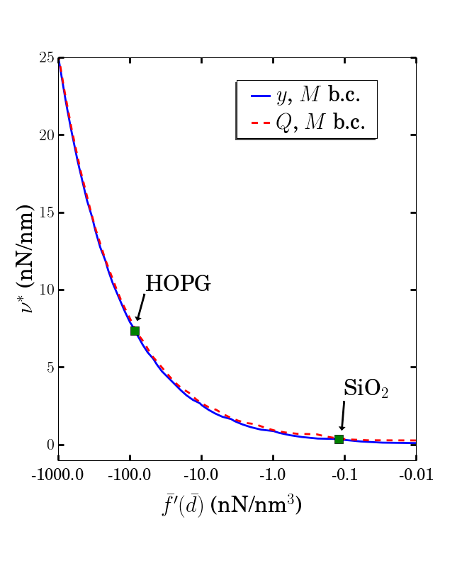
Figure 8: Buckling loads as a function of the derivative of the interaction force $\bar{f}$ at the equilibrium spacing $\bar{d}$. Both hinged and floating-edge boundary conditions are shown. For each case, $L=5$ nm and $\alpha=.16$ nN nm. The spacing on the horizontal axis is logarithmic.

The last figure in this section, Figure 9, shows how the limiting value of $\nu^{*}$ for large $L$ depends on $\alpha$. Figure 9 (a) is for graphene supported by SiO₂ and for $L=150$ nm. As one would expect, the figure indicates that for large $L$ the buckling load $\nu^{*}$ is the same for both hinged and floating-edge boundary conditions. The figure also shows that the buckling load increases as $\alpha$ increases, i.e., as the sheet gets stiffer. Figures 9 (b) corresponds to Figures 9 (a) but for graphene supported by a HOPG substrate.

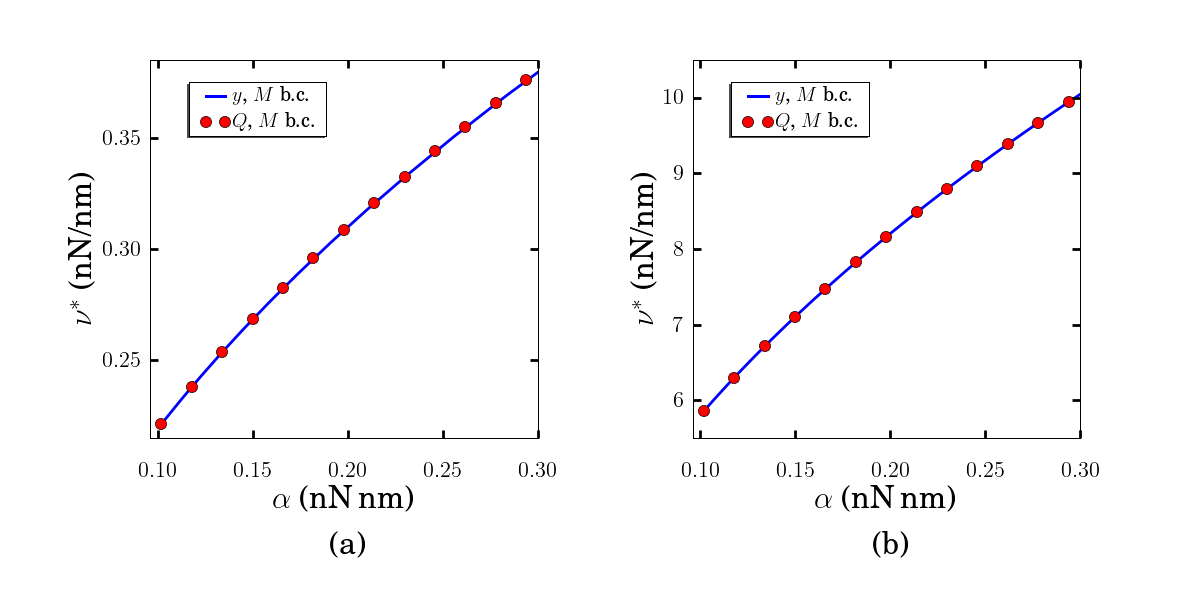
Figure 9: Buckling loads as a function of $\alpha$. Figure (a) is for graphene supported by SiO₂ and Figure (b) is for graphene supported by HOPG. In both cases, $L=150$ nm.

	SiO2				HOPG
	Hinged		Floating		Hinged		Floating
$L$	min	max	min	max	min	max	min	max
Near $5$ nm	0.2770	0.3462	0.4010	0.4617	7.3354	7.4008	7.5417	7.5682
Near $25$ nm	0.2770	0.2795	0.2848	0.2858	7.3354	7.3379	7.3448	7.3456
Near $150$ nm	0.2770	0.2771	0.2774	0.2774	7.3354	7.3355	7.3358	7.3358

Table 1: Summary of Buckling Loads. The min (max) value corresponds to the buckling load at the local minimum (maximum) nearest to the length $L$ on the graph of $\nu^{*}$ as a function of $L$. The numbers in the table have units of nN/nm.

The results of this section are summarized in Table 1

4 Post-Buckling Behavior

In this section we describe the post-buckling behavior predicted by our model. We present numerical results computed using the bifurcation software AUTO [5].

Figure 10 depicts a part of the bifurcation diagram for a sheet of length $L=30.4$ nm supported by a HOPG substrate with hinged boundary conditions. (Note that the dashed lines are used for clarity and not to indicate that the branches are unstable.) The variable on the vertical axis, which measures the size of solutions, is the angle $\theta(0)$ between the $\mathbf{i}$-axis and the tangent line at the left end of the sheet. The diagram shows a portion of the trivial branch containing the buckling load $\nu^{*}$ and the next two critical loads. There is a pitchfork bifurcation at $\nu^{*}$. The next two critical loads correspond to transcritical bifurcations. We also observe secondary bifurcations on the upper and lower branches emanating from the third critical load. Figure 10 should be compared to Figure 11(b) in [17] to illustrate the effect of the supporting substrate on the mechanical response of the graphene sheet.

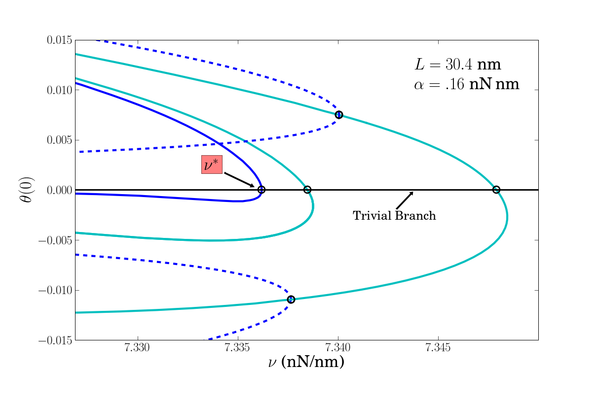
Figure 10: Bifurcation diagram for graphene supported by a HOPG substrate with hinged boundary conditions. $L=30.4$ nm. The first bifurcation is a pitchfork. The dashed lines are used for clarity and not to indicate unstable branches.

In Figure 11, we illustrate a possible post-buckling path based upon the bifurcation diagram in Figure 10. We assume the sheet undergoes a quasi-static loading process in which a compressive edge load is slowly increased from the unloaded configuration. For loads below the buckling load, the trivial branch is stable and the sheet remains flat. We assume that at the buckling load the trivial branch loses stability. Because the pitchfork opens to the left, if the load is further increased the solution must jump to a different branch. For macroscopic structures, this type of jump is often referred to as snap-buckling.

Determining rigorously to which branch the solution jumps entails analyzing the stability of branches by considering an appropriate potential energy for (2.1), (2.2) or by studying the dynamical version of these governing equations. Here we do not undertake this analysis. (See [32] for a stability analysis based on minimizing potential energy in a related problem.) However, to illustrate one possibility, we show the solution jumping to the lower branch of the upper pitchfork in Figure 10. The solution follows this branch until the secondary bifurcation point on the upper branch emanating from the third critical load in Figure 10. If the load is further increased, another snap-buckling may occur. The shapes of buckled solutions are depicted on the right in Figure 11. Note that both $x$ and $y$ are rescaled to be dimensionless.

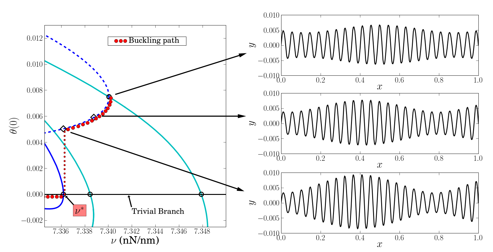
Figure 11: Possible buckling path. On the left is a part of the bifurcation diagram shown in Figure 10. One possible post-buckling path is indicated. On the right are the shapes of the buckled solutions along this path. The variables $x$ and $y$ are rescaled to be dimensionless.

Figure 12 depicts a part of the bifurcation diagram for a sheet of length $L=30.8$ nm supported by a HOPG substrate with hinged boundary conditions. (Here also the dashed lines are used for clarity and not to indicate that the branches are unstable.) The diagram shows a portion of the trivial branch containing the buckling load $\nu^{*}$ and the next two critical loads. The bifurcation at $\nu^{*}$ is transcritical. The next two critical loads correspond to pitchfork bifurcations. There are secondary bifurcations on the upper and lower branches emanating from the second critical load. In Figure 13, we illustrate a possible post-buckling path based upon the bifurcation diagram in Figure 12. For loads below the buckling load, the trivial branch is stable and the sheet remains flat. At the buckling load the trivial branch loses stability. The solution follows the lower branch from the transcritical bifurcation until a turning point is reached. If the load is further increased the sheet undergoes a snap-buckling and the solution jumps to a different branch. For example, the solution could jump to the lower branch of the upper pitchfork in Figure 12. The solution follows this branch until the secondary bifurcation point on the upper branch emanating from the second critical load. If the load is further increased, another snap-buckling may occur. The shapes of buckled solutions are depicted on the right. Both $x$ and $y$ are rescaled to be dimensionless.

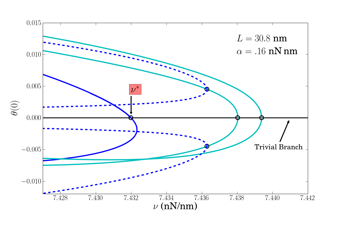
Figure 12: Bifurcation diagram for graphene supported by a HOPG substrate with hinged boundary conditions. $L=30.8$ nm. The first bifurcation is transcritical. The dashed lines are used for clarity and not to indicate unstable branches.

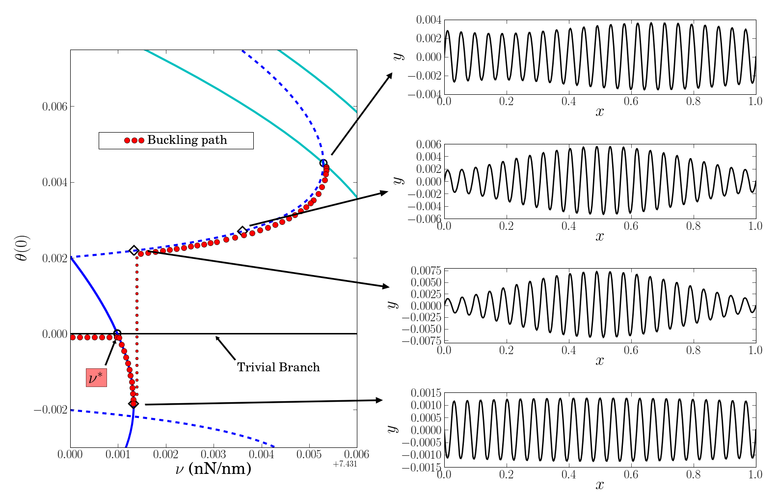
Figure 13: Possible post-buckling path. On the left is a part of the bifurcation diagram shown in Figure 12. One possible post-buckling path is indicated. On the right are the shapes of the buckled solutions along this path. The variables $x$ and $y$ are rescaled to be dimensionless.

The main point of the numerical results in this section is to illustrate the possibility of snap-buckling. This possibility suggests that the sheet, if loaded beyond the buckling load, would undergo a rapid and relatively large deformation from the flat configuration. As noted in the introduction, recent experimental and theoretical work on graphene establishes a connection between the deformation of the sheet and its transport properties. Hence our modeling predicts that at the buckling load the sheet could undergo a large, rapid change in transport properties. This property could be exploited in the design of nanoscale devices that incorporate graphene sheets.

5 Conclusion

In this paper we developed a nonlinear continuum model of a graphene sheet supported by a flat rigid substrate and loaded on a pair of opposite edges. We modeled the cross-section of the sheet as an elastica. Using techniques from bifurcation theory, we investigated how the buckling of the sheet depends on the boundary conditions, the composition of the substrate, and the length of the sheet. We also presented numerical results that illustrate some of the possible post-buckling behavior of the sheet. An interesting feature of the post-buckling behavior is that the sheet undergoes snap-buckling, which may have implications for the design of nanoscale devices that use graphene.

In our model, we assume the substrate is perfectly flat, which of course is not the case. For example, a substrate like SiO₂ may have undulations, and several recent papers suggest that graphene supported by an SiO₂ substrate will form ripples to follow these undulations [4, 11]. Within the context of our continuum modeling, ripples that form in the sheet prior to loading can be described as initial imperfections. A well-developed branch of bifurcation theory addresses how the presence of such imperfections influences buckling and post-buckling behavior. The study of this question follows naturally from the work presented here.

In a second variation of the problem modeled above, we can assume that the graphene sheet is deposited on a deformable, rather than rigid, substrate. Hence the cross-section of the substrate could be modeled as a beam with mechanical properties different from the sheet. This problem is motivated by recent experimental work in which graphene sheets are deposited on substrates of various compositions and strain is induced in the graphene by deforming the substrate [20, 21, 25].

This work was supported by NSF under grant number DMS-0407361.

References

- [1] S. S. Antman. Nonlinear Problems of Elasticity. Springer, 2005.
- [2] P. Blake, E. W. Hill, A. H. Castro Neto, K. S. Novoselov, D. Jiang, R. Yang, T. J. Booth, and A. K. Geim. Making graphene visible. Applied Physics Letters, 91(6):063124, 2007.
- [3] J. Scott Bunch, Arend M. van der Zande, Scott S. Verbridge, Ian W. Frank, David M. Tanenbaum, Jeevak M. Parpia, Harold G. Craighead, and Paul L. McEuen. Electromechanical Resonators from Graphene Sheets. Science, 315(5811):490–493, 2007.
- [4] A. Deshpande, W. Bao, F. Miao, C. N. Lau, and B. J. LeRoy. Spatially resolved spectroscopy of monolayer graphene on sio[sub 2]. Physical Review B (Condensed Matter and Materials Physics), 79(20):205411, 2009.
- [5] E. Doedel, A. R. Champneys, T. Fairgrieve, Y. Kuznetsov, B. Oldeman, R. Paffenroth, B. Sandstede, X. Wang, and C. Zhang. Auto-07p: Continuation and bifurcation software for ordinary differential equations. Technical report, Concordia University, http://indy.cs.concordia.ca/auto/, 2006.
- [6] A. Fasolino, J. H. Los, and M. I. Katsnelson. Intrinsic ripples in graphene. Nat Mater, 6(11):858–861, Nov 2007.
- [7] Doron Gazit. Theory of the spontaneous buckling of doped graphene. Physical Review B (Condensed Matter and Materials Physics), 79(11):113411, 2009.
- [8] A. K. Geim and K. S. Novoselov. The rise of graphene. Nature Materials, 6(3):183 – 191, 2007.
- [9] V. Geringer, M. Liebmann, T. Echtermeyer, S. Runte, M. Schmidt, R. Rückamp, M. C. Lemme, and M. Morgenstern. Intrinsic and extrinsic corrugation of monolayer graphene deposited on sio[sub 2]. Physical Review Letters, 102(7):076102, 2009.
- [10] L.A. Girifalco and R.A. Lad. Energy of cohesion, compressibility, and the potential energy functions of the graphite system. J. Chem. Phys., 25(4):693–697, 1956.
- [11] M. Ishigami, J.H. Chen, W.G. Cullen, M.S. Fuhrer, and E.D. Williams. Atomic structure of graphene on sio2. Nano Letters, 7(6):1643–1648, 2007.
- [12] Kim, Eun-Ah and Castro Neto, A. H. Graphene as an electronic membrane. EPL, 84(5):57007, dec 2008.
- [13] Kevin R. Knox, Shancai Wang, Alberto Morgante, Dean Cvetko, Andrea Locatelli, Tevfik Onur Mentes, Miguel Angel Nino, Philip Kim, and Jr. R. M. Osgood. Spectromicroscopy of single and multilayer graphene supported by a weakly interacting substrate. Physical Review B (Condensed Matter and Materials Physics), 78(20):201408, 2008.
- [14] T. Lenosky, X. Gonze, M. Teter, and V. Elser. Energetics of negatively curved graphitic carbon. Nature, 355:333–335, 1992.
- [15] Chunyu Li and Tsu-Wei Chou. A structural mechanics approach for the analysis of carbon nanotubes. International Journal of Solids and Structures, 40(10):2487 – 2499, 2003.
- [16] Teng Li and Zhao Zhang. Snap-through instability of graphene on substrates. Nanoscale Research Letters, 5(1):169–173, Jan 2010.
- [17] Q. Lu and R. Huang. nonlinear mechanics of single-atomic-layer graphene sheets. Int. J. Applied Mechanics, 1(3):443–467, 2009.
- [18] Xuekun Lu, Minfeng Yu, Hui Huang, and Rodney S Ruoff. Tailoring graphite with the goal of achieving single sheets. Nanotechnology, 10(3):269–272, 1999.
- [19] Jannik C. Meyer, A. K. Geim, M. I. Katsnelson, K. S. Novoselov, T. J. Booth, and S. Roth. The structure of suspended graphene sheets. Nature, 446(7131):60–63, Mar 2007.
- [20] Z. H. Ni, W. Chen, X. F. Fan, J. L. Kuo, T. Yu, A. T. S. Wee, and Z. X. Shen. Raman spectroscopy of epitaxial graphene on a sic substrate. Physical Review B (Condensed Matter and Materials Physics), 77(11):115416, 2008.
- [21] Zhen Hua Ni, Ting Yu, Yun Hao Lu, Ying Ying Wang, Yuan Ping Feng, and Ze Xiang Shen. Uniaxial strain on graphene: Raman spectroscopy study and band-gap opening. ACS Nano, 2(11):2301–2305, Oct 2008. doi: 10.1021/nn800459e.
- [22] R. Nicklow, N. Wakabayashi, and H. G. Smith. Lattice dynamics of pyrolytic graphite. Phys. Rev. B, 5(12):4951–4962, Jun 1972.
- [23] K. S. Novoselov, A. K. Geim, S. V. Morozov, D. Jiang, Y. Zhang, S. V. Dubonos, I. V. Grigorieva, and A. A. Firsov. Electric Field Effect in Atomically Thin Carbon Films. Science, 306(5696):666–669, 2004.
- [24] K.S. Novoselov, D. Jiang, F. Schedin, T.J. Booth, V.V. Khotkevich, S.V. Morozov, and A.K. Geim. Two-dimensional atomic crystals. Proceedings of the National Academy of Sciences, 102:10451–10453, 2005.
- [25] Vitor M. Pereira and A. H. Castro Neto. Strain engineering of graphene’s electronic structure. Physical Review Letters, 103(4):046801, 2009.
- [26] S. C. Pradhan and T. Murmu. Small scale effect on the buckling of single-layered graphene sheets under biaxial compression via nonlocal continuum mechanics. Computational Materials Science, 47(1):268–274, Nov 2009. doi: DOI: 10.1016/j.commatsci.2009.08.001.
- [27] M. A. Rafiee, J. Rafiee, Z.-Z. Yu, and N. Koratkar. Buckling resistant graphene nanocomposites. Applied Physics Letters, 95(22):223103, 2009.
- [28] D. H. Robertson, D. W. Brenner, and J. W. Mintmire. Energetics of nanoscale graphitic tubules. Physical Review B, 45(21):12592–12595, 1992.
- [29] H.-V. Roy, C. Kallinger, B. Marsen, and K. Sattler. Manipulation of graphitic sheets using a tunneling microscope. Journal of Applied Physics, 83(9):4695–4699, 1998.
- [30] C.Q. Ru. Column buckling of multiwalled carbon nanotubes with interlayer radial displacements. Phys. Rev. B, 62(24):16962–16967, 2000.
- [31] C.Q. Ru. Axially compressed buckling of a doublewalled carbon nanotube embedded in an elastic medium. J. Mech. Phys. Solids, 49:1265–1279, 2001.
- [32] S.D. Ryan, D. Golovaty, and J.P. Wilber. The stability of a graphene sheet pushed into a rigid substrate. Preprint (2010).
- [33] J. Sabio, C. Seoánez, S. Fratini, F. Guinea, A. H. Castro Neto, and F. Sols. Electrostatic interactions between graphene layers and their environment. Physical Review B (Condensed Matter and Materials Physics), 77(19):195409, 2008.
- [34] A. Sakhaee-Pour. Elastic buckling of single-layered graphene sheet. Computational Materials Science, 45(2):266 – 270, 2009.
- [35] Hannes C. Schniepp, Konstantin N. Kudin, Je-Luen Li, Robert K. Prud’homme, Roberto Car, Dudley A. Saville, and Ilhan A. Aksay. Bending properties of single functionalized graphene sheets probed by atomic force microscopy. ACS Nano, 2(12):2577–2584, 2008.
- [36] H.C. Schniepp, J.-L. Li, M.J. McAllister, H. Sai, M. Herrera-Alonso, D.H. Adamson, R.K. Prud’homme, R. Car, D.A. Saville, and I.A. Aksay. Functionalized single graphene sheets derived from splitting graphite oxide. J. Phys. Chem. B, 110(17):8535–8539, 2006.
- [37] Hui-Shen Shen. Postbuckling prediction of double-walled carbon nanotubes under hydrostatic pressure. International J. of Solids and Struct., 41(15):2643–2657, October 2004.
- [38] G.J. Simitses and D.H. Hodges. Fundamentals of Structural Stability. Elsevier, 2006.
- [39] Sasha Stankovich, Dmitriy A. Dikin, Geoffrey H. B. Dommett, Kevin M. Kohlhaas, Eric J. Zimney, Eric A. Stach, Richard D. Piner, SonBinh T. Nguyen, and Rodney S. Ruoff. Graphene-based composite materials. Nature, 442:282–286, 2006.
- [40] Elena Stolyarova, Kwang Taeg Rim, Sunmin Ryu, Janina Maultzsch, Philip Kim, Louis E. Brus, Tony F. Heinz, Mark S. Hybertsen, and George W. Flynn. High-resolution scanning tunneling microscopy imaging of mesoscopic graphene sheets on an insulating surface. Proceedings of the National Academy of Sciences, 104(22):9209–9212, 2007.
- [41] J. Tersoff. Energies of fullerenes. Phys. Rev. B, 46(23):15546–15549, Dec 1992.
- [42] R. C. Thompson-Flagg, M. J. B. Moura, and M. Marder. Rippling of graphene. EPL (Europhysics Letters), 85(4):46002, 2009.
- [43] S.P. Timoshenko and J.M. Gere. Theory of Elastic Stability. Mcgraw-Hill, 1961.
- [44] Zhan-chun Tu and Zhong-can Ou-Yang. Single-walled and multiwalled carbon nanotubes viewed as elastic tubes with the effective young’s moduli dependent on layer number. Phys. Rev. B, 65(23):233407, Jun 2002.
- [45] J.P. Wilber, A. Buldum, C.B. Clemons, D.D. Quinn, and G.W. Young. Continuum and atomistic modeling of interacting graphene layers. Phys. Rev. B, 75:045418, 2007.
- [46] B.I. Yakobson, C.J. Brabec, and J. Bernholc. Nanomechanics of carbon nanotubes: Instabilities beyond the linear response. Phys. Rev. Letters, 76:2511–2514, 1996.
- [47] Jianfeng Zhou, Ziyong Shen, Shimin Hou, Xingyu Zhao, Zengquan Xue, Zujin Shi, and Zhennan Gu. Adsorption and manipulation of carbon onions on highly oriented pyrolytic graphite studied with atomic force microscopy. Applied Surface Science, 253(6):3237 – 3241, 2007.