Exclusive rare $B_{s}\to(K,\eta,\eta^{\prime})\ell^{+}\ell^{-}$ decays in the light-front quark model

Abstract

Using the light-front quark model, we calculate the transition form factors, decay rates, and longitudinal lepton polarization asymmetries for the exclusive rare $B_{s}\to(K,\eta^{(\prime)})(\ell^{+}\ell^{-},\nu_{\ell}\bar{\nu_{\ell}}$ ($\ell=e,\mu,\tau$) decays within the standard model, taking into account the $\eta-\eta^{\prime}$ mixing angle. For the mixing angle $\theta=-20^{\circ}$ ($-10^{\circ}$) in the octet-singlet basis, we obtain ${\rm BR}(B_{s}\to\eta\sum\nu_{\ell}\bar{\nu}_{\ell})=1.1\;(1.7)\times 10^{-6}$, ${\rm BR}(B_{s}\to\eta\mu^{+}\mu^{-})=1.5\;(2.4)\times 10^{-7}$, ${\rm BR}(B_{s}\to\eta\tau^{+}\tau^{-})=3.8\;(5.8)\times 10^{-8}$, ${\rm BR}(B_{s}\to\eta^{\prime}\sum\nu_{\ell}\bar{\nu}_{\ell})=1.8\;(1.3)\times 10^{-6}$, ${\rm BR}(B_{s}\to\eta^{\prime}\mu^{+}\mu^{-})=2.4\;(1.8)\times 10^{-7}$, and ${\rm BR}(B_{s}\to\eta^{\prime}\tau^{+}\tau^{-})=3.4\;(2.6)\times 10^{-8}$, respectively. The branching ratios for the $B_{s}\to K(\nu_{\ell}\bar{\nu_{\ell}},\ell^{+}\ell^{-})$ decays are at least an order of magnitude smaller than those for the $B_{s}\to\eta^{(\prime)}(\nu_{\ell}\bar{\nu_{\ell}},\ell^{+}\ell^{-})$ decays. The averaged values of the lepton polarization asymmetries for $B_{s}\to(K,\eta^{(\prime)})\ell^{+}\ell^{-}$ are obtained as $\langle P^{K}_{L}\rangle_{\mu}=\langle P^{\eta}_{L}\rangle_{\mu}=\langle P^{\eta^{\prime}}_{L}\rangle_{\mu}=-0.98$, $\langle P^{K}_{L}\rangle_{\tau}=-0.24$, $\langle P^{\eta}_{L}\rangle_{\tau}=-0.20$ and $\langle P^{\eta^{\prime}}_{L}\rangle_{\tau}=-0.14$, respectively.

1 Introduction

The study of the exclusive decays in the beauty sector allows one to explore the standard model (SM) and search for new physics effects. The B factory experiments such as BaBar at SLAC, Belle at KEK, LHCb at CERN, and B-TeV at Fermilab make precision tests of the SM and beyond the SM ever more promising. Especially, the $B_{s}$-meson system becomes a key element in the $B$-physics program of B factories ever since the first evidence for $B_{s}$ production at the $\Upsilon(5S)$ was found by the CLEO collaboration [1, 2]. The D0 [3] and CDF [4] Collaborations have made measurements of the charge-parity (CP) violating weak $B_{s}-\bar{B}_{s}$ mixing phase $\phi_{s}$ in $B_{s}\to J/\psi\phi$ decays. While the SM expectation $\phi^{\rm SM}_{s}$ [5, 6] is nearly zero, the measured $\phi_{s}$ differs from 0 by more than $3\sigma$ (but with a sizable error). This measurement of $\phi_{s}$ inconsistent with zero (if confirmed) would indicate an evidence of new physics. Recently, the Belle Collaboration also measured the branching ratios of the $B_{s}\to J/\psi\phi$ and $B_{s}\to J/\psi\eta$ decays and the preliminary result [7] of the $B_{s}\to J/\psi\phi$ decay is about 3 times larger than that for the $B_{s}\to J/\psi\eta$ decay. This ratio agrees with a rough estimate obtained within the naive quark model (neglect octet-singlet mixing), where the $s\bar{s}$ part of the $\eta$ meson wave function is one third in contrast to the fully $s\bar{s}$ content of $\phi$ mesons. With the upcoming chances that a numerous number of $B_{s}$ mesons will be produced at hadron colliders, one might explore the exclusive rare $B_{s}$ decays to $(K,\eta,\eta^{\prime})\ell^{+}\ell^{-}$(and $\nu_{\ell}\bar{\nu}_{\ell}$) ($\ell=e,\mu,\tau$) induced by the flavor-changing neutral current (FCNC) transitions $b\to(d,s)$. Since in the SM the rare $B_{s}$ decays are forbidden at tree level and occur at the lowest order only through one-loop penguin diagrams [8, 9, 10, 11, 12, 13, 14, 15], the rare $B_{s}$ decays are well suited to test the SM and detect new physics effects. While the experimental tests of exclusive decays are much easier than those of inclusive ones, the theoretical understanding of exlcusive decays is complicated mainly due to the nonperturbative hadronic form factors entered in the long distance nonperturbative contributions. Therefore, a reliable estimate of the hadronic form factors for the exclusive rare $B_{s}$ decays is very important to make correct predictions within and beyond the SM. The $\eta-\eta^{\prime}$ mixing angle may also be extracted from the rare $B_{s}$ decays to $\eta$ and $\eta^{\prime}$ final states.

In our previous work [16], we have analyzed the exclusive rare $B\to K\ell^{+}\ell^{-}$ decays within the framework of the SM, using our light-front quark model (LFQM) based on the QCD-motivated effective LF Hamiltonian [17, 18, 19]. The experimental values of the branching ratios ${\rm BR}(B\to K\ell^{+}\ell^{-})=(0.75^{+0.25}_{-0.21}\pm 0.09)\times 10^{-6}$ from Belle [20] and $(0.34\pm 0.07\pm 0.02)\times 10^{-6}$ ($\ell=e,\mu$) from BABAR [21] detectors are consistent with our LFQM prediction $0.5\times 10^{-6}$ [16] based on the SM. Recently, we also analyzed $B_{c}$ properties and various exclusive decay modes such as the semileptonic $B_{c}\to(D,\eta_{c},B,B_{s})\ell\nu_{\ell}$ decays [22], the rare $B_{c}\to D_{(s)}\ell^{+}\ell^{-}$ [23], and the nonleptonic two-body $B_{c}\to(D_{(s)},\eta_{c},B_{(s)})(P,V)$ decays [24] (here $P$ and $V$ denote pseudoscalar and vector mesons, respectively). The form factors $f_{\pm}(q^{2})$ and $f_{T}(q^{2})$ for the exclusive rare decays [23] between two pseudoscalar mesons are obtained in the Drell-Yan-West ($q^{+}=q^{0}+q^{3}=0$) frame [25] (i.e., $q^{2}=-{\bf q}^{2}_{\perp}<0$), which is useful because only the valence contributions are needed unless the zero-mode contribution exists. The covariance (i.e., frame independence) of our model has been checked by performing the LF calculation in the $q^{+}=0$ frame in parallel with the manifestly covariant calculation using the exactly solvable covariant fermion field theory model in $(3+1)$ dimensions. We also found the zero-mode contribution to the form factor $f_{-}(q^{2})$ and identified [22] the zero-mode operator that is convoluted with the initial and final state LF wave functions.

The purpose of this paper is to extend our our LFQM [16, 17, 18, 19, 22, 23, 24] to calculate the hadronic form factors, decay rates and the longitudinal lepton polarization asymmetries (LPAs) for the exclusive rare $B_{s}\to(K,\eta,\eta^{\prime})\ell^{+}\ell^{-}$ and $\nu_{\ell}\bar{\nu}_{\ell}$ decays within the SM. The LPA, as another parity-violating observable, is an important asymmetry [26] and could be measured at hadron colliders such as LHCb. In particular, the $\tau$ channel would be more accessible experimentally than $e$- or $\mu$-channels since the LPAs in the SM are known to be proportional to the lepton mass. There are some theoretical approaches to the calculations of the exclusive rare $B_{s}\to\eta\ell^{+}\ell^{-}$ [27, 28, 29] and $B_{s}\to\eta^{\prime}\ell^{+}\ell^{-}$ [28, 29] decays, but not the $B_{s}\to K\ell^{+}\ell^{-}$ decay mode as far as we know.

The paper is organized as follows. In Sec. 2, the SM operator basis, describing the $b\to(d,s)(\ell^{+}\ell^{-},\nu_{\ell}\bar{\nu}_{\ell})$ transitions, is presented. In Sec. 3, we briefly describe the formulation of our LFQM and the procedure of fixing the model parameters using the variational principle for the QCD motivated effective Hamiltonian. We discuss the rare decays between two pseudoscalar mesons using an exactly solvable model based on the covariant Bethe-Salpeter (BS) model of $(3+1)$-dimensional fermion field theory and show the equivalence between the results obtained by the manifestly covariant method and the LF method in the $q^{+}=0$ frame. We then present the LF covariant forms of the form factors $f_{\pm}(q^{2})$ and $f_{T}(q^{2})$ obtained from our LFQM. The $\eta-\eta^{\prime}$ mixing angle for the $B_{s}\to\eta^{(\prime)}$ transitions is also discussed in this section. In Sec. 4, our numerical results, i.e. the form factors, decay rates, and the LPAs for the rare $B_{s}\to(K,\eta,\eta^{\prime})(\ell^{+}\ell^{-},\nu_{\ell}\bar{\nu}_{\ell})$ decays are presented. Summary and discussion of our main results follow in Sec. 5.

2 Effective Hamiltonian

In the SM, the exclusive rare $B_{s}\to P_{q}(\ell^{+}\ell^{-},\nu_{\ell}\bar{\nu}_{\ell})$ ($q=d,s$) decays are at the quark level described by the loop $b\to q\;(\ell^{+}\ell^{-},\nu_{\ell}\bar{\nu}_{\ell})$ transitions, and receive contributions from the $Z(\gamma)$-penguin and $W$-box diagrams as shown in Fig. 1.

Figure 1: Loop diagrams for $B_{s}\to P_{q}(\ell^{+}\ell^{-},\nu_{\ell}\bar{\nu}_{\ell})(q=d,s)$ transitions.

The effective Hamiltonian responsible for the $b\to q\ell^{+}\ell^{-}\;(q=d,s)$ decay processes can be represented in terms of the Wilson coefficients, $C_{7}^{\rm eff},C_{9}^{\rm eff}$ and $C_{10}$ as [9]

$${\cal H}^{\ell^{+}\ell^{-}}_{\rm eff} = \frac{G_{F}\alpha_{\rm em}}{2\sqrt{2}\pi}V_{tb}V^{*}_{tq}\biggl{[}C^{\rm eff}_{9}\bar{q}\gamma_{\mu}(1-\gamma_{5})b\bar{\ell}\gamma^{\mu}\ell+C_{10}\bar{q}\gamma_{\mu}(1-\gamma_{5})b\bar{\ell}\gamma^{\mu}\gamma_{5}\ell$$ (1)

$$-C_{7}^{\rm eff}\frac{2m_{b}}{q^{2}}\bar{q}i\sigma_{\mu\nu}q^{\nu}(1+\gamma_{5})b\bar{\ell}\gamma^{\mu}\ell\biggr{]},$$

where $G_{F}$ is the Fermi constant, $\alpha_{\rm em}$ is the fine structure constant, and $V_{ij}$ are the Cabibbo-Kobayashi-Maskawa (CKM) matrix elements. The relevant Wilson coefficients $C_{i}$ can be found in Ref. [9]. The effective Hamiltonian responsible for the $b\to q\nu_{\ell}\bar{\nu}_{\ell}\;(q=d,s)$ decay processes is given by [11, 12]

$${\cal H}^{\nu_{\ell}\bar{\nu}_{\ell}}_{\rm eff} = \frac{G_{F}\alpha_{\rm em}}{2\sqrt{2}\pi}V_{tb}V^{*}_{tq}\frac{X(x_{t})}{\sin^{2}\theta_{W}}\bar{q}\gamma_{\mu}(1-\gamma_{5})b\bar{\nu}_{\ell}\gamma^{\mu}(1-\gamma_{5})\nu_{\ell},$$ (2)

where $x_{t}=(m_{t}/M_{W})^{2}$ and $X(x_{t})$ is the top quark loop function [11, 12], which is given by

$$X(x)=\frac{x}{8}\biggl{(}\frac{2+x}{x-1}+\frac{3x-6}{(x-1)^{2}}\ln x\biggr{)}.$$ (3)

Besides the short distance (SD) contributions, the main effect on the decay comes from the long distance (LD) contributions due to the $c\bar{c}$ resonance states ($J/\psi,\psi^{\prime},\cdots$). The effective Wilson coefficient $C^{\rm eff}_{9}$ taking into account both the SD and LD contributions has the following form [9]

$$C^{\rm eff}_{9}(s)=C_{9}+Y_{SD}(s)+Y_{LD}(s),$$ (4)

where the explicit forms of $Y_{SD}(s)$ and $Y_{LD}(s)$ can be found in [9, 30]. For the LD contribution $Y_{LD}(s)$, we include two $c\bar{c}$ resonant states $J/\psi(1S)$ and $\psi^{\prime}(2S)$ and use $\Gamma(J/\psi\to\ell^{+}\ell^{-})=5.26\times 10^{-6}$ GeV, $M_{J/\psi}=3.1$ GeV, $\Gamma_{J/\psi}=87\times 10^{-6}$ GeV for $J/\psi(1S)$ and $\Gamma(\psi^{\prime}\to\ell^{+}\ell^{-})=2.12\times 10^{-6}$ GeV, $M_{\psi^{\prime}}=3.69$ GeV, $\Gamma_{\psi^{\prime}}=277\times 10^{-6}$ GeV for $\psi^{\prime}(2S)$ [31].

The LD contributions to the exclusive $B_{s}\to P_{q}\;(q=d,s)$ decays are contained in the meson matrix elements of the bilinear quark currents appearing in ${\cal H}^{\ell^{+}\ell^{-}}_{\rm eff}$ and ${\cal H}^{\nu_{\ell}\bar{\nu_{\ell}}}_{\rm eff}$. In the matrix elements of the hadronic currents for $B_{s}\to P_{q}$ transitions, the parts containing $\gamma_{5}$ do not contribute. Considering Lorentz and parity invariances, these matrix elements can be parametrized in terms of hadronic form factors as follows:

$$J^{\mu}\equiv\langle P_{q}|\bar{q}\gamma^{\mu}b|B_{s}\rangle=f_{+}(q^{2})P^{\mu}+f_{-}(q^{2})q^{\mu},$$ (5)

and

$$J^{\mu}_{T} \equiv \langle P_{q}|\bar{q}i\sigma^{\mu\nu}q_{\nu}b|B_{s}\rangle=\frac{f_{T}(q^{2})}{M_{B_{s}}+M_{P_{q}}}[q^{2}P^{\mu}-(M^{2}_{B_{s}}-M^{2}_{P_{q}})q^{\mu}],$$ (6)

where $P=P_{B_{s}}+P_{P_{q}}$ and $q=P_{B_{s}}-P_{P_{q}}$ is the four-momentum transfer to the lepton pair and $4m^{2}_{\ell}\leq q^{2}\leq(M_{B_{s}}-M_{P_{q}})^{2}$. We use the convention $\sigma^{\mu\nu}=(i/2)[\gamma^{\mu},\gamma^{\nu}]$ for the antisymmetric tensor. Sometimes it is useful to express Eq. (5) in terms of $f_{+}(q^{2})$ and $f_{0}(q^{2})$, which are related to the exchange of $1^{-}$ and $0^{+}$, respectively, and satisfy the following relations:

$$f_{+}(0)=f_{0}(0),\;f_{0}(q^{2})=f_{+}(q^{2})+\frac{q^{2}}{M^{2}_{B_{s}}-M^{2}_{P_{q}}}f_{-}(q^{2}).$$ (7)

With the help of the effective Hamiltonian in Eq. (1) and Eqs. (5) and (6), the transition amplitude ${\cal M}=\langle P_{q}\ell^{+}\ell^{-}|{\cal H}_{\rm eff}|B_{s}\rangle$ for the $B_{s}\to P_{q}\ell^{+}\ell^{-}$ decay can be written as

$${\cal M} = \frac{G_{F}\alpha_{\rm em}}{2\sqrt{2}\pi}V_{tb}V^{*}_{tq}\biggl{\{}\biggl{[}C^{\rm eff}_{9}J_{\mu}-\frac{2m_{b}}{q^{2}}C^{\rm eff}_{7}J^{T}_{\mu}\biggr{]}\bar{\ell}\gamma^{\mu}\ell+C_{10}J_{\mu}\bar{\ell}\gamma^{\mu}\gamma_{5}\ell\biggr{\}}.$$ (8)

The differential decay rate for $B_{s}\to P_{q}\ell^{+}\ell^{-}$ is given by [32, 33]

$$\frac{d\Gamma_{\ell\ell}}{ds} = \frac{M^{5}_{B_{s}}G^{2}_{F}}{3\cdot 2^{9}\pi^{5}}\alpha^{2}_{\rm em}|V_{tb}V^{*}_{tq}|^{2}\phi_{H}^{1/2}\biggl{(}1-\frac{4t}{s}\biggr{)}^{1/2}\biggl{[}\phi_{H}\biggl{(}1+\frac{2t}{s}\biggr{)}{\cal F}_{1}+12t{\cal F}_{2}\biggr{]},$$ (9)

where

$${\cal F}_{1} = \biggl{|}C^{\rm eff}_{9}f_{+}-\frac{2\hat{m_{b}}C^{\rm eff}_{7}}{1+\sqrt{r}}f_{T}\biggr{|}^{2}+|C_{10}f_{+}|^{2},$$

$${\cal F}_{2} = |C_{10}|^{2}\biggl{[}(1+r-\frac{s}{2})|f_{+}|^{2}+(1-r)f_{+}f_{-}+\frac{s}{2}|f_{-}|^{2}\biggr{]},$$

$$\phi_{H} = (s-1-r)^{2}-4r,$$ (10)

with $s=q^{2}/M^{2}_{B_{s}}$, $t=m^{2}_{\ell}/M^{2}_{B_{s}}$, $\hat{m_{b}}=m_{b}/M_{B_{s}}$ and $r=M^{2}_{P_{q}}/M^{2}_{B_{s}}$. Equation (9) may be written in terms of ($f_{+},f_{0},f_{T}$) instead of ($f_{+},f_{-},f_{T}$) as discussed in [16]. Note also from Eqs. (9) and (2) that the form factor $f_{-}(q^{2})$ does not contribute in the massless lepton limit.

The differential decay rate for $B_{s}\to P_{q}\nu_{\ell}\bar{\nu}_{\ell}$ can be easily obtained from the corresponding formula Eq. (9) for $B_{s}\to P_{q}\ell^{+}\ell^{-}$ by the replacement $\hat{m}_{\ell}\to 0$, $C_{7}^{\rm eff}\to 0$, and $C^{\rm eff}_{9}=-C_{10}\to X(x_{t})/\sin^{2}\theta_{W}$, i.e.

$$\frac{d}{ds}\sum_{\ell}\Gamma_{\nu_{\ell}{\bar{\nu}}_{\ell}} = 3\frac{M^{5}_{B_{s}}G^{2}_{F}}{3\cdot 2^{8}\pi^{5}\sin^{4}\theta_{W}}\alpha^{2}_{\rm em}|V_{tb}V^{*}_{tq}|^{2}\phi_{H}^{3/2}|X(x_{t})|^{2}|f_{+}|^{2},$$ (11)

where the factor of 3 in the numerator corresponds to the sum over the three neutrino flavors. Dividing Eqs. (9) and (11) by the total width of the $B_{s}$ meson, one can obtain the differential branching ratio $d{\rm BR}(B_{s}\to P_{q}\ell^{+}\ell^{-})/ds=(d\Gamma(B_{s}\to P_{q}\ell^{+}\ell^{-})/\Gamma_{\rm tot})/ds$. As another interesting observable, the LPA, is defined as

$$P_{L}(s)=\frac{d\Gamma_{h=-1}/ds-d\Gamma_{h=1}/ds}{d\Gamma_{h=-1}/ds+d\Gamma_{h=1}/ds},$$ (12)

where $h=+1(-1)$ denotes right (left) handed $\ell^{-}$ in the final state. From Eq. (9), one obtains for $B_{s}\to P_{q}\ell^{+}\ell^{-}$

$$P_{L}(s)=\frac{2\biggl{(}1-4\frac{t}{s}\biggr{)}^{1/2}\phi_{H}C_{10}f_{+}\biggl{[}f_{+}{\rm Re}C^{\rm eff}_{9}-\frac{2\hat{m_{b}}C^{\rm eff}_{7}}{1+\sqrt{r}}f_{T}\biggr{]}}{\biggl{[}\phi_{H}\biggl{(}1+2\frac{t}{s}\biggr{)}{\cal F}_{1}+12t{\cal F}_{2}\biggr{]}}.$$ (13)

Because of the experimental difficulties of studying the polarizations of each lepton depending on $s$ and the Wilson coefficients, it would be better to eliminate the dependence of the LPA on $s$, by considering the averaged form over the entire kinematical region. The averaged LPA is defined by

$$\langle P_{L}\rangle=\frac{\int^{(1-\sqrt{r})^{2}}_{4t}P_{L}\frac{dBR}{ds}ds}{\int^{(1-\sqrt{r})^{2}}_{4t}\frac{dBR}{ds}ds}.$$ (14)

3 Review of our LFQM

The key idea in our LFQM [17, 18, 22] for the ground state mesons is to treat the radial wave function as a trial function for the variational principle to the QCD-motivated effective Hamiltonian saturating the Fock state expansion by the constituent quark and antiquark. The QCD-motivated effective Hamiltonian for a description of the ground state meson mass spectra is given by

$$H_{q\bar{q}}=H_{0}+V_{q\bar{q}}=\sqrt{m^{2}_{q}+{\vec{k}}^{2}}+\sqrt{m^{2}_{\bar{q}}+{\vec{k}}^{2}}+V_{q\bar{q}},$$ (15)

where

$$V_{q\bar{q}}=V_{0}+V_{\rm hyp}=a+br^{n}-\frac{4\alpha_{s}}{3r}+\frac{2}{3}\frac{{\bf S}_{q}\cdot{\bf S}_{\bar{q}}}{m_{q}m_{\bar{q}}}\nabla^{2}V_{\rm coul}.$$ (16)

In this work, we use the Coulomb plus linear confining (i.e. $n=1$) potential together with the hyperfine interaction $\langle{\bf S}_{q}\cdot{\bf S}_{\bar{q}}\rangle=1/4\;(-3/4)$ for the vector (pseudoscalar) meson, which enables us to analyze the meson mass spectra and various wave-function-related observables, such as decay constants, electromagnetic form factors of mesons in a spacelike region, and the weak form factors for the exclusive semileptonic and rare decays of pseudoscalar mesons in the timelike region [16, 17, 18, 19, 22, 23, 24, 34, 35].

The momentum-space LF wave function of the ground state pseudoscalar mesons is given by $\Psi(x_{i},{\bf k}_{i\perp},\lambda_{i})={\cal R}_{\lambda_{1}\lambda_{2}}(x_{i},{\bf k}_{i\perp})\phi(x_{i},{\bf k}_{i\perp})$, where $\phi(x_{i},{\bf k}_{i\perp})$ is the radial wave function and ${\cal R}_{\lambda_{1}\lambda_{2}}$ is the covariant spin-orbit wave function. The model wave function is represented by the Lorentz-invariant variables, $x_{i}=p^{+}_{i}/P^{+}$, ${\bf k}_{i\perp}={\bf p}_{i\perp}-x_{i}{\bf P}_{\perp}$ and $\lambda_{i}$, where $P^{\mu}=(P^{+},P^{-},{\bf P}_{\perp})=(P^{0}+P^{3},(M^{2}+{\bf P}^{2}_{\perp})/P^{+},{\bf P}_{\perp})$ is the momentum of the meson $M$, and $p^{\mu}_{i}$ and $\lambda_{i}$ are the momenta and the helicities of constituent quarks, respectively.

The covariant form of the spin-orbit wave function for pseudoscalar mesons is given by

$${\cal R}_{\lambda_{1}\lambda_{2}} = \frac{-\bar{u}_{\lambda_{1}}(p_{1})\gamma_{5}v_{\lambda_{2}}(p_{2})}{\sqrt{2}\sqrt{M^{2}_{0}-(m_{1}-m_{2})^{2}}},$$ (17)

where $M^{2}_{0}=\sum_{i=1}^{2}({\bf k}^{2}_{i\perp}+m^{2}_{i})/x_{i}$ is the boost invariant meson mass square obtained from the free energies of the constituents in mesons. For the radial wave function $\phi$, we use the Gaussian wave function:

$$\phi(x_{i},{\bf k}_{i\perp})=\frac{4\pi^{3/4}}{\beta^{3/2}}\sqrt{\frac{\partial k_{z}}{\partial x}}{\rm exp}(-{\vec{k}}^{2}/2\beta^{2}),$$ (18)

where $\beta$ is the variational parameter. When the longitudinal component $k_{z}$ is defined by $k_{z}=(x-1/2)M_{0}+(m^{2}_{2}-m^{2}_{1})/2M_{0}$, the Jacobian of the variable transformation $\{x,{\bf k}_{\perp}\}\to{\vec{k}}=({\bf k}_{\perp},k_{z})$ is given by

$$\frac{\partial k_{z}}{\partial x}=\frac{M_{0}}{4x_{1}x_{2}}\biggl{\{}1-\biggl{[}\frac{m^{2}_{1}-m^{2}_{2}}{M^{2}_{0}}\biggr{]}^{2}\biggr{\}}.$$ (19)

The normalization factor in Eq. (18) is obtained from the following normalization of the total wave function:

$$\int^{1}_{0}dx\int\frac{d^{2}{\bf k}_{\perp}}{16\pi^{3}}|\Psi(x,{\bf k}_{i\perp})|^{2}=1.$$ (20)

We apply our variational principle to the QCD-motivated effective Hamiltonian first to evaluate the expectation value of the central Hamiltonian $H_{0}+V_{0}$, i.e., $\langle\phi|(H_{0}+V_{0})|\phi\rangle$, with a trial function $\phi(x_{i},{\bf k}_{i\perp})$ that depends on the variational parameter $\beta$. Once the model parameters are fixed by minimizing the expectation value $\langle\phi|(H_{0}+V_{0})|\phi\rangle$, the mass eigenvalue of each meson is obtained as $M_{q\bar{q}}=\langle\phi|(H_{0}+V_{q\bar{q}})|\phi\rangle$. Minimizing energies with respect to $\beta$ and searching for a fit to the observed ground state meson spectra, our central potential $V_{0}$ obtained from our optimized potential parameters ($a=-0.72$ GeV, $b=0.18$ GeV², and $\alpha_{s}=0.31$) [17] for the Coulomb plus linear potential was found to be quite comparable with the quark potential model suggested by Scora and Isgur [36], where they obtained $a=-0.81$ GeV, $b=0.18$ GeV², and $\alpha_{s}=0.3\sim 0.6$ for the Coulomb plus linear confining potential. A more detailed procedure for determining the model parameters of light- and heavy-quark sectors can be found in our previous works [17, 18]. Our model parameters $(m_{q},\beta_{q\bar{q}})$ obtained from the linear potential model relevant to this work are summarized in Table 1. The predictions of the ground state meson mass spectra can be found in [22]. We should note that our model parameters ($m,\beta$) automatically satisfies the normalization of the total wave function and were fixed by the variational principle to the QCD-motivated effective Hamiltonian. Those parameters in turn automatically satisfies the normalization of the electromagnetic form factors at $q^{2}=0$ and every other physical observables obtained from our LFQM such as decay constants and electroweak form factors are the predictions. This distinguishes our LFQM from other quark model.

Table 1: The constituent quark masses[GeV] and the Gaussian parameters $\beta$[GeV] obtained from the linear potential in [18], which are necessary for $B_{s}\to(K,\eta,\eta^{\prime})$ decay modes. $q=u$ and $d$.

$m_{q}$	$m_{s}$	$m_{b}$	$\beta_{qs}$	$\beta_{ss}$	$\beta_{sb}$
0.22	0.45	5.2	0.3886	0.4128	0.5712

3.1 Form factors for the rare $B_{s}\to P$ decays in our LFQM

Most popular phenomenological LFQM uses the Gaussian wave function as the radial wave function due to its predictive power of various physical observables. However, since the LFQM using the Gaussian wave function does not have a counterpart of manifestly covariant model, it is hard to check the covariance of the model. To check the covariance of LFQM, one can start from the manifestly covariant field theory model. For example, using the exactly solvable covariant BS model of (3+1)-dimensional fermion field theory [37, 38, 39], one can perform the LF calculation in parallel with the manifestly covariant calculation and compare the results from the two models. Comparing the LF results and the manifestly covariant results, we were able to derive the LF covariant form factors between two pseudoscalar meson explicitly and to analyze the zero-mode complication. Since the detailed procedure of finding LF covariant transition form factors ($f_{+},f_{-},f_{T}$) was already given in our previous works [22, 23], we shall briefly describe the essential procedure of obtaining the LF covariant form factors from the exactly solvable covariant BS model of (3+1)-dimensional fermion field theory and show the results of the LF covariant form factors.

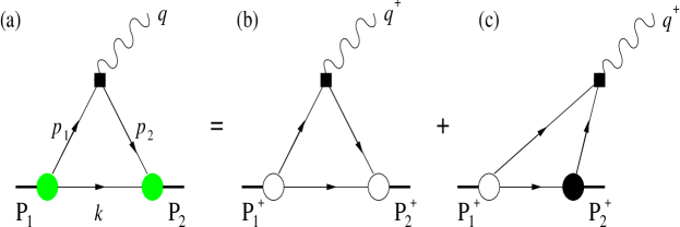
Figure 2: The covariant diagram (a) corresponds to the sum of the LF valence diagram (b) defined in $0<k^{+}<P^{+}_{2}$ region and the nonvalence diagram (c) defined in $P^{+}_{2}<k^{+}<P^{+}_{1}$ region. The large white and black blobs at the meson-quark vertices in (b) and (c) represent the ordinary LF wave functions and the non-wave-function vertex, respectively. The small black box at the quark-gauge boson vertex indicates the insertion of the relevant Wilson operator.

The covariant diagram shown in Fig. 2(a) is in general equivalent to the sum of the LF valence diagram 2(b) and the nonvalence diagram 2(c). The matrix element $J^{\mu}_{(T)}$ obtained from the covariant diagram of Fig. 2(a) is given by

$$J^{\mu}_{(T)}=ig_{1}g_{2}\Lambda^{2}_{1}\Lambda^{2}_{2}\int\frac{d^{4}k}{(2\pi)^{4}}\frac{S^{\mu}_{(T)}}{N_{\Lambda_{1}}N_{1}N_{k}N_{2}N_{\Lambda_{2}}},$$ (21)

where $g_{1}$ and $g_{2}$ are the normalization factors which can be fixed by requiring both charge form factors of pseudoscalar mesons to be unity at zero momentum transfer, respectively. To regularize the covariant fermion triangle-loop in (3+1) dimensions, we replace the point gauge-boson vertex $\gamma^{\mu}$ by a non-local smearing gauge-boson vertex $({\Lambda_{1}}^{2}/N_{\Lambda_{1}})\gamma^{\mu}({\Lambda_{2}}^{2}/N_{\Lambda_{2}})$, where $N_{\Lambda_{1}}=p_{1}^{2}-{\Lambda_{1}}^{2}+i\epsilon$ and $N_{\Lambda_{2}}=p_{2}^{2}-{\Lambda_{2}}^{2}+i\epsilon$, and thus the factor $({\Lambda_{1}}{\Lambda_{2}})^{2}$ appears in the normalization factor. $\Lambda_{1}$ and $\Lambda_{2}$ play the role of momentum cut-offs similar to the Pauli-Villars regularization [37]. Our replacement of $\gamma^{\mu}$ by the non-local smearing gauge-boson vertex remedies the conceptual difficulty associated with the asymmetry appearing if the fermion loop were regulated by smearing the $q\bar{q}$ bound-state vertex. The rest of the denominators in Eq. (21), i.e., $N_{1}N_{k}N_{2}$, are coming from the intermediate fermion propagators in the triangle loop diagram and are given by

$$N_{k}=k^{2}-m^{2}+i\epsilon,\;N_{j}=p_{j}^{2}-{m_{j}}^{2}+i\epsilon\;(j=1,2),$$ (22)

where $m_{1}$, $m$, and $m_{2}$ are the masses of the constituents carrying the intermediate four-momenta $p_{1}=P_{1}-k$, $k$, and $p_{2}=P_{2}-k$, respectively. Furthermore, the trace terms $S^{\mu}$ from the vector current and $S^{\mu}_{T}$ from the tensor current are given by

$$S^{\mu} = {\rm Tr}[\gamma_{5}(\not\!p_{1}+m_{1})\gamma^{\mu}(\not\!p_{2}+m_{2})\gamma_{5}(-\not\!k+m)]$$ (23)

$$= 4\{p^{\mu}_{1}(p_{2}\cdot k+m_{2}m)+p^{\mu}_{2}(p_{1}\cdot k+m_{1}m)+k^{\mu}(m_{1}m_{2}-p_{1}\cdot p_{2})\},$$

and

$$S^{\mu}_{T} = {\rm Tr}[\gamma_{5}(\not\!p_{1}+m_{1})i\sigma^{\mu\nu}q_{\nu}(\not\!p_{2}+m_{2})\gamma_{5}(-\not\!k+m)]$$ (24)

$$= -4\{p^{\mu}_{1}[m(p_{2}\cdot q)+m_{2}(k\cdot q)]-p^{\mu}_{2}[m(p_{1}\cdot q)+m_{1}(k\cdot q)]$$

$$+k^{\mu}[m_{1}(p_{2}\cdot q)-m_{2}(p_{1}\cdot q)]\},$$

respectively. By doing the integration over $k^{-}$ in Eq. (21), one finds the two LF time-ordered contributions to the residue calculations corresponding to the two poles in $k^{-}$, the LF valence contribution [Fig. 2(b)] defined in $0<k^{+}<P^{+}_{2}$ region and the nonvalence contribution [Fig. 2(c)] defined in $P^{+}_{2}<k^{+}<P^{+}_{1}$ region. The nonvalence contribution [Fig. 2(c)] in the $q^{+}>0$ frame corresponds to the zero mode (if it exists) in the $q^{+}\to 0$ limit [40]. Performing the LF calculation of Eq. (21) in the $q^{+}=0$ frame in parallel with the manifestly covariant calculation, we use the plus component of the currents to obtain the form factors $f_{+}(q^{2})$ and $f_{T}(q^{2})$. For the form factor $f_{-}(q^{2})$, we use both the plus and perpendicular components of the currents. As we have shown in [22, 23], while the form factors $f_{+}(q^{2})$ and $f_{T}(q^{2})$ can be obtained only from the valence contribution in the $q^{+}=0$ frame without encountering the zero-mode contribution, the form factor $f_{-}(q^{2})$ receives the zero mode. In our recent analysis of semileptonic $B_{c}$ decays [22], we identified the zero-mode operator that is convoluted with the initial and final state LF valence wave functions to generate the zero-mode contribution to the form factor $f_{-}(q^{2})$ in the $q^{+}=0$ frame. Our method can also be realized effectively by the method presented by Jaus [39] using the orientation of the LF plane characterized by the invariant equation $\omega\cdot x=0$, where $\omega$ is an arbitrary light-like four vector. More detailed analysis of the zero-mode operator and the LF covariance of the form factors $f_{\pm}$ and $f_{T}$ can be found in [22, 23]. While the manifestly covariant BS model of fermion field theory model is good for the qualitative analysis of the exclusive rare decays, it is still semi-realistic. We thus replace the LF vertex functions in the BS model with the more phenomenological Gaussian radial wave functions in our LFQM since the zero-mode operator is independent from the choice of radial wave function as discussed in [22].

The LF covariant form factors $f_{\pm}(q^{2})$ and $f_{T}(q^{2})$ for $B_{s}(q_{1}\bar{q})\to P(q_{2}\bar{q})$ transitions obtained from the $q^{+}=0$ frame are given by (see  [22, 23] for more detailed derivations)

$$f_{+}(q^{2})=\int^{1}_{0}dx\int\frac{d^{2}{\bf k}_{\perp}}{16\pi^{3}}\frac{\phi_{1}(x,{\bf k}_{\perp})}{\sqrt{{\cal A}_{1}^{2}+{\bf k}^{2}_{\perp}}}\frac{\phi_{2}(x,{\bf k}^{\prime}_{\perp})}{\sqrt{{\cal A}_{2}^{2}+{\bf k}^{\prime 2}_{\perp}}}({\cal A}_{1}{\cal A}_{2}+{\bf k}_{\perp}\cdot{\bf k^{\prime}}_{\perp}),$$ (25)

$$f_{-}(q^{2}) = \int^{1}_{0}(1-x)dx\int\frac{d^{2}{\bf k}_{\perp}}{16\pi^{3}}\frac{\phi_{1}(x,{\bf k}_{\perp})}{\sqrt{{\cal A}^{2}_{1}+{\bf k}^{2}_{\perp}}}\frac{\phi_{2}(x,{\bf k^{\prime}}_{\perp})}{\sqrt{{\cal A}^{2}_{2}+{\bf k}^{\prime 2}_{\perp}}}\biggl{\{}-x(1-x)M^{2}_{1}$$ (26)

$$-{\bf k}^{2}_{\perp}-m_{1}m+(m_{2}-m){\cal A}_{1}+2\frac{q\cdot P}{q^{2}}\biggl{[}{\bf k}^{2}_{\perp}+2\frac{({\bf k}_{\perp}\cdot{\bf q}_{\perp})^{2}}{q^{2}}\biggr{]}$$

$$+2\frac{({\bf k}_{\perp}\cdot{\bf q}_{\perp})^{2}}{q^{2}}+\frac{{\bf k}_{\perp}\cdot{\bf q}_{\perp}}{q^{2}}[M^{2}_{2}-(1-x)(q^{2}+q\cdot P)+2xM^{2}_{0}$$

$$-(1-2x)M^{2}_{1}-2(m_{1}-m)(m_{1}+m_{2})]\biggr{\}},$$

$$f_{T}(q^{2}) = (M_{1}+M_{2})\int^{1}_{0}(1-x)dx\int\frac{d^{2}{\bf k}_{\perp}}{16\pi^{3}}\frac{\phi_{1}(x,{\bf k}_{\perp})}{\sqrt{{\cal A}^{2}_{1}+{\bf k}^{2}_{\perp}}}\frac{\phi_{2}(x,{\bf k^{\prime}}_{\perp})}{\sqrt{{\cal A}^{2}_{2}+{\bf k}^{\prime 2}_{\perp}}}$$ (27)

$$\times\biggl{[}{\cal A}_{1}-(m_{1}-m_{2})\frac{{\bf k}_{\perp}\cdot{\bf q}_{\perp}}{q^{2}}\biggr{]},$$

where ${\bf k^{\prime}}_{\perp}={\bf k}_{\perp}+(1-x){\bf q}_{\perp}$, ${\cal A}_{i}=(1-x)m_{i}+xm$ ($i=1,2$), and $q\cdot P=M^{2}_{1}-M^{2}_{2}$ with $M_{1}$ and $M_{2}$ being the physical masses of the initial and final state mesons, respectively. Our results for the form factors given by Eqs. (25)-(27) are essentially the same as those presented in [41]. We should note that the LF covariant form factor $f_{-}(q^{2})$ in Eq. (26) is the sum of the valence contribution $f^{\rm val}_{-}(q^{2})$ and the zero-mode contribution $f^{\rm Z.M.}_{-}(q^{2})$ [22]. Since the form factors $f_{\pm}(q^{2})$ and $f_{T}(q^{2})$ are defined in the spacelike ($q^{2}=-{\bf q}^{2}_{\perp}<0$) region, we then analytically continue them to the timelike $q^{2}>0$ region by changing ${\bf q}_{\perp}^{2}$ to $-q^{2}$ in the form factors. We also compare our analytic solutions with the double pole parametric form given by

$$f_{i}(q^{2})=\frac{f_{i}(0)}{1-\sigma_{1}s+\sigma_{2}s^{2}},$$ (28)

where $\sigma_{1}$ and $\sigma_{2}$ are the fitted parameters.

3.2 $\eta-\eta^{\prime}$ mixing for the $B_{s}\to\eta^{(\prime)}$ decays

In this subsection, we discuss the $\eta-\eta^{\prime}$ mixing to obtain the $B_{s}\to\eta^{(\prime)}$ transition form factors. The octet-singlet mixing angle $\theta$ of $\eta$ and $\eta^{\prime}$ is known to be in the range of $-10^{\rm o}$ to $-23^{\rm o}$ [31]. The physical $\eta$ and $\eta^{\prime}$ are the mixtures of the flavor $SU(3)$ octet $\eta_{8}$ and singlet $\eta_{0}$ states:

$$\left(\begin{array}[]{cc}\eta\\ \eta^{\prime}\end{array}\,\right)=\left(\begin{array}[]{cc}\cos\theta\;\;-\sin\theta\\ \sin\theta\;\;\;\;\;\cos\theta\end{array}\,\right)\left(\begin{array}[]{c}\eta_{8}\\ \eta_{0}\end{array}\,\right),$$ (29)

where $\eta_{8}=(u\bar{u}+d\bar{d}-2s\bar{s})/\sqrt{6}$ and $\eta_{0}=(u\bar{u}+d\bar{d}+s\bar{s})/\sqrt{3}$. Analogously, in terms of the quark-flavor(QF) basis $\eta_{q}=(u\bar{u}+d\bar{d})/\sqrt{2}$ and $\eta_{s}=s\bar{s}$, one obtains [42]

$$\left(\begin{array}[]{cc}\eta\\ \eta^{\prime}\end{array}\,\right)=\left(\begin{array}[]{cc}\cos\phi\;\;-\sin\phi\\ \sin\phi\;\;\;\;\;\cos\phi\end{array}\,\right)\left(\begin{array}[]{c}\eta_{q}\\ \eta_{s}\end{array}\,\right).$$ (30)

The two schemes are equivalent to each other by $\phi=\theta+\arctan\sqrt{2}$ when ${\rm SU}_{f}(3)$ symmetry is perfect. Although it was frequently assumed that the decay constants follow the same pattern of state mixing, the mixing properties of the decay constants will generally be different from those of the meson state since the decay constants only probe the short-distance properties of the valence Fock states while the state mixing refers to the mixing of the overall wave function [42].

Defining $\langle P(p)|J^{q(s)}_{\mu 5}|0\rangle=-if^{q(s)}_{P}p^{\mu}$ ($P=\eta,\eta^{\prime}$) in the QF basis, the four parameters $f^{q}_{P}$ and $f^{s}_{P}$ can be expressed in terms of two mixing angles ($\phi_{q}$ and $\phi_{s}$) and two decay constants ($f_{q}$ and $f_{s}$), i.e. [42],

$$\left(\begin{array}[]{cc}f^{q}_{\eta}\;\;\;\;\;f^{s}_{\eta}\\ f^{q}_{\eta^{\prime}}\;\;\;\;\;f^{s}_{\eta^{\prime}}\end{array}\,\right)=\left(\begin{array}[]{cc}\cos\phi_{q}\;\;-\sin\phi_{s}\\ \sin\phi_{q}\;\;\;\;\;\cos\phi_{s}\end{array}\,\right)\left(\begin{array}[]{cc}f_{q}\;\;0\\ 0\;\;\;f_{s}\end{array}\,\right).$$ (31)

The difference between the mixing angles $\phi_{q}-\phi_{s}$ is due to the Okubo-Zweig-Iizuka(OZI)-violating effects [43] and is found to be small ($\phi_{q}-\phi_{s}<5^{\circ}$). The OZI rule implies that the difference between $\phi_{q}$ and $\phi_{s}$ vanishes (i.e., $\phi_{q}=\phi_{s}=\phi$) to leading order in the $1/N_{c}$ expansion. Similarly, the four parameters $f^{8}_{P}$ and $f^{0}_{P}$ in the octet-singlet basis may be written in terms of two angles ($\theta_{8}$ and $\theta_{0}$) and two decay constants ($f_{8}$ and $f_{0}$). However, in this case, $\theta_{8}$ and $\theta_{0}$ turn out to differ considerably and become equal only in the ${\rm SU}_{f}(3)$ symmetry limit [42, 44].

We shall use the QF basis with the single mixing angle $\phi$ to analyze the $B_{s}\to\eta^{(\prime)}$ decay modes. In this case, a generic form factor $F$ and the branching ratio for the $B_{s}\to\eta^{(\prime)}$ are given by

$$F^{B_{s}\to\eta(\eta^{\prime})}=-\sin\phi(\cos\phi)F^{B_{s}\to\eta_{s}},$$ (32)

with the physical $\eta^{(\prime)}$ mass and

$${\rm BR}[B_{s}\to\eta(\eta^{\prime})\ell^{+}\ell^{-}]=\sin^{2}\phi(\cos^{2}\phi){\rm BR}[B_{s}\to\eta_{s}\ell^{+}\ell^{-}],$$ (33)

respectively. Recently, the KLOE Collaboration [45] extracted the pseudoscalar mixing angle $\phi$ in the QF basis by measuring the ratio ${\rm BR}(\phi\to\eta^{\prime}\gamma)/{\rm BR}(\phi\to\eta\gamma)$. The measured values are $\phi=(39.7\pm 0.7)^{\circ}$ and $(41.5\pm 0.3_{\rm stat}\pm 0.7_{\rm syst}\pm 0.6_{\rm th})^{\circ}$ with and without the gluonium content for $\eta^{\prime}$, respectively. However, since the mixing angle for $\eta-\eta^{\prime}$ is still a controversial issue, we use unspecified value for $\phi$ rather than adopting some specific value.

4 Numerical results

In our numerical calculations for the exclusive rare $B_{s}\to(K,\eta,\eta^{\prime})(\nu_{\ell}\bar{\nu_{\ell}},\ell^{+}\ell^{-})$ decays, we use the model parameters ($m_{q},\beta$) for the linear confining potential given in Table 1. Although our predictions [22] of ground state heavy meson masses are overall in good agreement with the experimental values, we use the experimental meson masses [31] in the computations of the decay widths to reduce possible theoretical uncertainties.

Note that in the numerical calculations we take $(m_{c},m_{b})=(1.8,5.2)$ GeV in all formulas except in the Wilson coefficient $C^{\rm eff}_{9}$, where $(m_{c},m_{b,\rm pole})=(1.4,4.8)$ GeV have been commonly used [9]. For the numerical values of the Wilson coefficients, we use the results given by Ref. [9]:

$$C_{1} = -0.248,\;C_{2}=1.107,\;C_{3}=0.011,$$

$$C_{4} = -0.026,\;C_{5}=0.007,\;C_{6}=-0.031,$$

$$C^{\rm eff}_{7} = -0.313,\;C_{9}=4.344,\;C_{10}=-4.669,$$ (34)

and other input parameters are $|V_{tb}V^{*}_{ts}|=0.039$, $|V_{tb}V^{*}_{td}|=0.008$, $\alpha_{\rm em}^{-1}=129$, $M_{W}=80.43$ GeV, $m_{t}=171.3$ GeV, $\sin^{2}\theta_{W}=0.2233$, and $\tau_{B^{0}_{s}}=1.470$ ps.

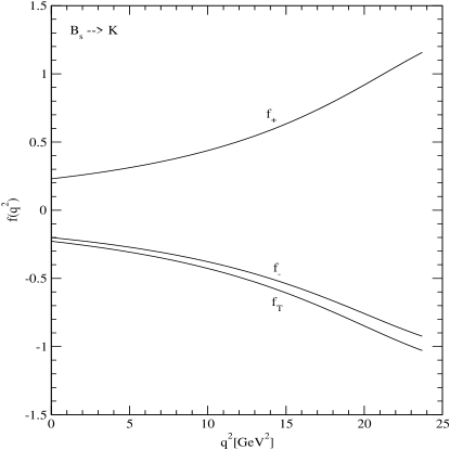
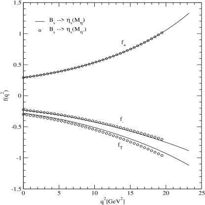
Figure 3: The weak form factors for $B_{s}\to K$(left panel) and $B_{s}\to\eta_{s}$(right panel) decays, respectively.

Table 2: Results for form factors at $q^{2}=0$ of $B_{s}\to(K,\eta,\eta^{\prime})$ transition and parameters $\sigma_{i}$ defined in Eq. (28). The coefficients in $\eta$ and $\eta^{\prime}$ represent quark mixing angles, i.e. $c_{\eta}=-\sin\phi$ and $c_{\eta^{\prime}}=\cos\phi$, respectively.

Mode	$f_{+}(0)$	$\sigma_{1}$	$\sigma_{2}$	$f_{-}(0)$	$\sigma_{1}$	$\sigma_{2}$	$f_{T}(0)$	$\sigma_{1}$	$\sigma_{2}$
$B_{s}\to K$	0.230	$-1.650$	0.822	$-0.201$	$-1.638$	0.835	$-0.228$	$-1.633$	0.835
$B_{s}\to\eta$	$0.291c_{\eta}$	$-1.574$	0.751	$-0.231c_{\eta}$	$-1.582$	0.825	$-0.280c_{\eta}$	$-1.561$	0.782
$B_{s}\to\eta^{\prime}$	$0.291c_{\eta^{\prime}}$	$-1.575$	0.770	$-0.225c_{\eta^{\prime}}$	$-1.570$	0.835	$-0.300c_{\eta^{\prime}}$	$-1.561$	0.802

In Fig. 3, we show the $q^{2}$ dependences of the form factors $f_{\pm}(q^{2})$ and $f_{T}(q^{2})$ for the $B_{s}\to K$ (left panel) and $B_{s}\to\eta_{s}$ with physical masses of $\eta$ and $\eta^{\prime}$ (right panel), respectively. The form factors at $q^{2}=0$ and the parameters $\sigma_{i}$ of the double pole form defined in Eq. (28) are listed in Table 2. The form factor $f_{+}(q^{2})$ for the $B_{s}\to\eta_{s}$ has the same $q^{2}$ dependence (apart from the mixing angle $\phi$) for both $\eta$ (solid line) and $\eta^{\prime}$ (circle) since $f_{+}$ does not depend on the daughter meson mass as one can see from Eq. (25). On the other hand, the form factors $f_{-}$ and $f_{T}$ between $\eta$ and $\eta^{\prime}$ are slightly different (apart from the mixing angle $\phi$) since they involve the daughter meson mass as one can see from Eqs. (26) and  (27). The form factors at the zero recoil point (i.e., $q^{2}=q^{2}_{\rm max})$ correspond to the overlap integral of the initial and final state meson wave functions. The maximum recoil point (i.e., $q^{2}=0$) corresponds to a final state meson recoiling with the maximum three-momentum $|{\vec{P}}_{f}|=(M^{2}_{B_{s}}-M^{2}_{f})/2M_{B_{s}}$ in the rest frame of the $B_{s}$ meson. As a sensitivity check of our LFQM, we find for the $B_{s}\to K$ transition that our form factors are changed only about 3$\%$ as the light $d$-quark mass varies about 20$\%$. This indicates that the transition form factors for $b\to d$ decay processes are quite stable on the variation of $d$ quark mass. The form factors for the $B_{s}\to\eta_{s}$ have also been computed by Geng and Liu [28] using the similar LFQM but only with the valence contributions in the purely longitudinal $q^{+}\neq 0$ frame. Although the form factors $f_{+}$ and $f_{T}$ at the maximum recoil point obtained from [28] do not receive nonvalence contributions, they receive nonvalence contributions at other nonzero $q^{2}$ values. The nonvalence contributions to $f_{-}$ are more serious for the entire $q^{2}$ range including the $q^{2}=0$ point. For instance, $f_{-}$ obtained from [28](see Fig. 2 in [28]) shows a sharp increasing as $q^{2}$ near the zero recoil point in contrast to our result. This indicates the nonvalence contribution to $f_{-}$ is quite large, which in particular overestimate the branching ratio for the $\tau$ dilepton decay mode. Although the form factor $f_{-}(q^{2})$ does not contribute to the branching ratio in the massless lepton ($\ell=e$ or $\mu$) decay, it is important for the heavy $\tau$ decay process.

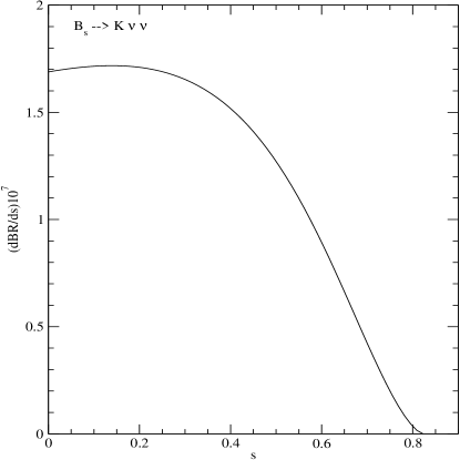
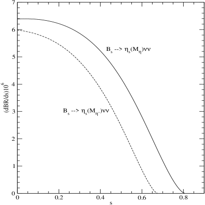
Figure 4: Differential branching ratios for $B_{s}\to K\sum\nu_{\ell}\bar{\nu_{\ell}}$ (left panel) and $B_{s}\to\eta_{s}\sum\nu_{\ell}\bar{\nu_{\ell}}$ (right panel) decays, respectively.

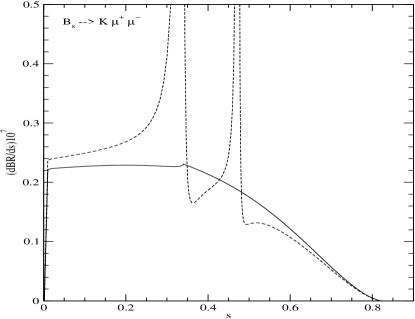
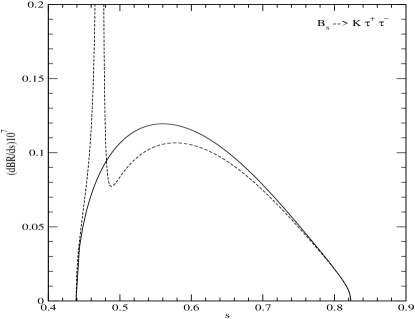
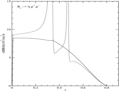
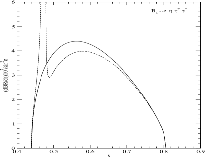
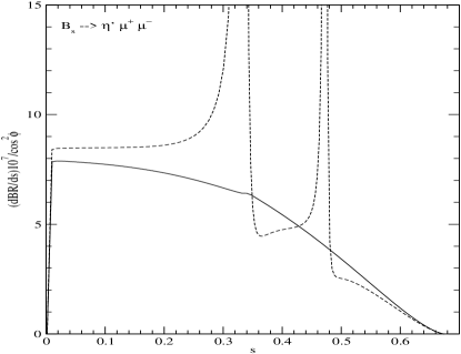
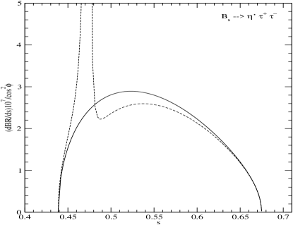
Figure 5: Differential branching ratios for $B_{s}\to K\ell^{+}\ell^{-}$ (upper panel) and $B_{s}\to\eta\ell^{+}\ell^{-}$ (middle panel) and $B_{s}\to\eta^{\prime}\ell^{+}\ell^{-}$ (lower panel) with $\ell=\mu$ and $\tau$, respectively. The solid and dashed lines represent the results without and with the LD contributions, respectively.

We show our results for the differential branching ratios for $B_{s}\to(K,\eta_{s})\sum\nu_{\ell}\bar{\nu}_{\ell}$ with physical masses of $\eta$ and $\eta^{\prime}$ in Fig. 4 and $B_{s}\to(K,\eta,\eta^{\prime})\ell^{+}\ell^{-}$ ($\ell=\mu$ and $\tau$) in Fig. 5, respectively. For the $B_{s}\to(K,\eta,\eta^{\prime})\ell^{+}\ell^{-}$ transitions in Fig. 5, the solid (dashed) lines represent the results without (with) the LD contribution to $C^{\rm eff}_{9}$. Since the $B_{s}\to K$ is induced by $b\to d$ transition compared to the $B_{s}\to\eta_{s}$ induced by $b\to s$ at the quark level, the branching ratios for the final $K$ meson are order of magnitude smaller than the corresponding branching ratios for the final $\eta$ meson. For the $B_{s}\to(K,\eta,\eta^{\prime})\ell^{+}\ell^{-}$ decays (see Fig. 5), the LD contributions (dashed lines) clearly overwhelm the nonresonant branching ratios near $J/\psi(1S)$ and $\psi^{\prime}(2S)$ peaks, however, suitable $\ell^{+}\ell^{-}$ invariant mass cuts can separate the LD contribution from the SD one away from these peaks. This divides the spectrum into two distinct regions [26, 46]: (i) low-dilepton mass, $4m^{2}_{\ell}\leq q^{2}\leq M^{2}_{J/\psi}-\delta$, and (ii) high-dilepton mass, $M^{2}_{\psi^{\prime}}+\delta\leq q^{2}\leq q^{2}_{\rm max}$, where $\delta$ is to be matched to an experimental cut.

Our predictions for the nonresonant branching ratios are summarized in Table 3 with general form of the mixing angle $\phi$ in the QF basis. Our results are also compared with other theoretical predictions such as the LF and constituent QM [28] and the QCD sum rules (SR) [29] within the SM. Since the amplitude $B_{s}\to(K,\eta,\eta^{\prime})\ell^{+}\ell^{-}$ is regular at $q^{2}=0$, the transitions $B_{s}\to(K,\eta,\eta^{\prime})e^{+}e^{-}$ and $B_{s}\to(K,\eta,\eta^{\prime})\mu^{+}\mu^{-}$ have almost the same decay rates, i.e. insensitive to the mass of the light lepton. Our predictions of branching ratios are close to the QCD SR results [29] but a bit smaller than the LFQM results [28]. But the results from [28] could be lowered if the nonvalence contributions are properly taken into account. For the mixing angle $\theta=-20^{\circ}$ ($-10^{\circ}$) in the octet-singlet basis, which corresponds to $\phi=34.74^{\circ}$ ($44.74^{\circ}$) in the QF basis, we obtain ${\rm BR}(B_{s}\to\eta\sum\nu_{\ell}\bar{\nu}_{\ell})=1.1\;(1.7)\times 10^{-6}$, ${\rm BR}(B_{s}\to\eta\mu^{+}\mu^{-})=1.5\;(2.4)\times 10^{-7}$, ${\rm BR}(B_{s}\to\eta\tau^{+}\tau^{-})=3.8\;(5.8)\times 10^{-8}$, ${\rm BR}(B_{s}\to\eta^{\prime}\sum\nu_{\ell}\bar{\nu}_{\ell})=1.8\;(1.3)\times 10^{-6}$, ${\rm BR}(B_{s}\to\eta^{\prime}\mu^{+}\mu^{-})=2.4\;(1.8)\times 10^{-7}$, and ${\rm BR}(B_{s}\to\eta^{\prime}\tau^{+}\tau^{-})=3.4\;(2.6)\times 10^{-8}$, respectively.

It is also worth comparing the branching ratios between $B_{s}\to K$ and $B_{s}\to\eta$, which may be written as

$$\frac{{\rm BR}(B_{s}\to K\mu^{+}\mu^{-})}{{\rm BR}(B_{s}\to\eta\mu^{+}\mu^{-})}=\frac{1}{\sin^{2}\phi}\biggl{|}\frac{V_{td}}{V_{ts}}\biggr{|}^{2}(1-\Delta_{SU(3)}),$$ (35)

where the $SU(3)$ correction term $\Delta_{SU(3)}$ is estimated about $0.3$ in our model calculation. Such a kind of relation may be further scrutinized by considering an additional correction term neglected in the effective Hamiltonian as discussed in [29]. The branching ratios with the LD contributions for $B_{s}\to(K,\eta,\eta^{\prime})\ell^{+}\ell^{-}$ $(\ell=\mu,\tau)$ are also presented in Table 4 for low- and high-dilepton mass regions of $q^{2}$.

Table 3: Nonresonant branching ratios (in units of $10^{-7}$) for $B_{s}\to(K,\eta,\eta^{\prime})\sum\nu_{\ell}\bar{\nu}_{\ell}$ and $B_{s}\to(\eta,\eta^{\prime})\ell^{+}\ell^{-}$ transitions compared with other theoretical model predictions within the SM.

Mode	This work	[28]	[29]
$B_{s}\to K\sum\nu_{\ell}\bar{\nu}_{\ell}$	1.01
$B_{s}\to\eta\sum\nu_{\ell}\bar{\nu}_{\ell}$	$35.1\sin^{2}\phi$	$58.3\sin^{2}\phi$(LFQM)	$(21.6\pm 4.6)\sin^{2}\phi$(set A)
		$54.1\sin^{2}\phi$(CQM)	$(50.1\pm 15.9)\sin^{2}\phi$(set B)
$B_{s}\to\eta^{\prime}\sum\nu_{\ell}\bar{\nu}_{\ell}$	$26.2\cos^{2}\phi$	$42.1\cos^{2}\phi$(LFQM)	$(16.0\pm 3.6)\cos^{2}\phi$ (set A)
		$39.7\cos^{2}\phi$(CQM)	$(33.9\pm 8.9)\cos^{2}\phi$ (set B)
$B_{s}\to K\mu^{+}\mu^{-}$	0.14
$B_{s}\to\eta\mu^{+}\mu^{-}$	$4.75\sin^{2}\phi$	$8.53\sin^{2}\phi$(LFQM)	$(2.73\pm 0.68)\sin^{2}\phi$(set A)
		$7.78\sin^{2}\phi$(CQM)	$(5.92\pm 1.59)\sin^{2}\phi$ (set B)
$B_{s}\to\eta^{\prime}\mu^{+}\mu^{-}$	$3.53\cos^{2}\phi$	$6.06\cos^{2}\phi$(LFQM)	$(1.96\pm 0.53)\cos^{2}\phi$(set A)
		$5.69\cos^{2}\phi$(CQM)	$(3.92\pm 1.07)\cos^{2}\phi$ (set B)
$B_{s}\to K\tau^{+}\tau^{-}$	0.03
$B_{s}\to\eta\tau^{+}\tau^{-}$	$1.17\sin^{2}\phi$	$1.67\sin^{2}\phi$(LFQM)	$(0.68\pm 0.11)\sin^{2}\phi$(set A)
		$1.67\sin^{2}\phi$(CQM)	$(1.82\pm 0.34)\sin^{2}\phi$ (set B)
$B_{s}\to\eta^{\prime}\tau^{+}\tau^{-}$	$0.51\cos^{2}\phi$	$0.83\cos^{2}\phi$(LFQM)	$(0.28\pm 0.05)\cos^{2}\phi$(set A)
		$0.72\cos^{2}\phi$(CQM)	$(0.69\pm 0.13)\cos^{2}\phi$ (set B)

Table 4: Branching ratios with the LD contributions for $B_{c}\to(D,D_{s})\ell^{+}\ell^{-}$ for low and high dilepton mass regions of $q^{2}$ [GeV²] obtained from the linear (HO) potential parameters.

Mode	$4m^{2}_{\ell}\leq q^{2}\leq 8.5$	$14.5\leq q^{2}\leq q^{2}_{\rm max}$
$B_{s}\to K\mu^{+}\mu^{-}$	$7.72\;(6.63)\times 10^{-9}$	$2.27\;(2.62)\times 10^{-9}$
$B_{s}\to K\tau^{+}\tau^{-}$		$2.43\;(2.66)\times 10^{-9}$
$B_{s}\to\eta\mu^{+}\mu^{-}$	$2.86\;(2.44)\sin^{2}\phi\times 10^{-7}$	$7.00\;(8.10)\sin^{2}\phi\times 10^{-8}$
$B_{s}\to\eta\tau^{+}\tau^{-}$		$9.13\;(9.85)\sin^{2}\phi\times 10^{-8}$
$B_{s}\to\eta^{\prime}\mu^{+}\mu^{-}$	$2.54\;(2.17)\cos^{2}\phi\times 10^{-7}$	$2.54\;(2.13)\cos^{2}\phi\times 10^{-8}$
$B_{s}\to\eta^{\prime}\tau^{+}\tau^{-}$		$3.42\;(3.67)\cos^{2}\phi\times 10^{-8}$

In Fig. 6, we show the LPAs for $B\to(K,\eta,\eta^{\prime})\ell^{+}\ell^{-}$ ($\ell=\mu,\tau$) as a function of $s$. In both $\mu$ and $\tau$ dilepton decays, the LPAs become zero at the end point regions of $s$. However, we note that if $m_{\ell}=0$, the LPAs are not zero at the end points. As in the case of the $B\to K\mu^{+}\mu^{-}$ [16, 33, 32, 47] and $B_{c}\to D_{(s)}\mu^{+}\mu^{-}$ [23] decays where $P_{L}\simeq-1$ away from the end point regions, the LPAs away from the end point regions are also close to $-1$ for the $B_{s}\to(K,\eta,\eta^{\prime})\mu^{+}\mu^{-}$ transitions. In fact, the $P_{L}$ for the muon decay is insensitive to the form factors, e.g. our $P_{L}$ away from the end point regions is well approximated by [47]

$$P_{L}\simeq 2\frac{C_{10}{\rm Re}C^{\rm eff}_{9}}{|C^{\rm eff}_{9}|^{2}+|C_{10}|^{2}}\simeq-1,$$ (36)

in the limit of $C^{\rm eff}_{7}\to 0$ from Eq. (13). It also shows that the $P_{L}$ for the $\mu$ dilepton channel is insensitive to the little variation of $C^{\rm eff}_{7}$ as expected. On the other hand, the LPA for the $\tau$ dilepton channel is sensitive to the form factors. Similar observation has also been made in our recent work for $B_{c}\to(D,D_{s})\ell^{+}\ell^{-}$ decays [23].

The averaged values $\langle P^{K,\eta^{(\prime)}}_{L}\rangle_{\ell}$ of the LPAs for $B_{s}\to(K,\eta^{(\prime)})\ell^{+}\ell^{-}$ without the LD contributions are $\langle P^{K}_{L}\rangle_{\mu}=\langle P^{\eta}_{L}\rangle_{\mu}=\langle P^{\eta^{\prime}}_{L}\rangle_{\mu}=-0.98$, $\langle P^{K}_{L}\rangle_{\tau}=-0.24$, $\langle P^{\eta}_{L}\rangle_{\tau}=-0.20$ and $\langle P^{\eta^{\prime}}_{L}\rangle_{\tau}=-0.14$, respectively.

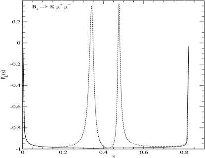
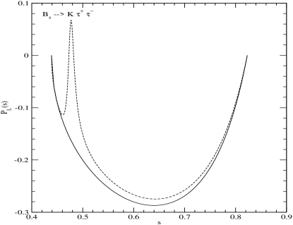
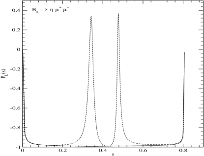
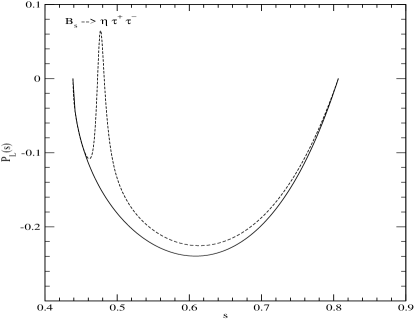
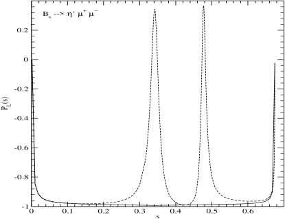
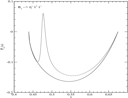
Figure 6: Longitudinal lepton polarization asymmetries for $B_{s}\to K\ell^{+}\ell^{-}$(upper panel), $B_{s}\to\eta\ell^{+}\ell^{-}$(middle panel) and $B_{s}\to\eta^{\prime}\ell^{+}\ell^{-}$(lower panel). The same line codes are used as in Fig. 5.

5 Summary and Discussion

In this work, we investigated the exclusive rare semileptonic $B_{s}\to(K,\eta,\eta^{\prime})(\nu_{\ell}\bar{\nu_{\ell}},\ell^{+}\ell^{-})$ ($\ell=e,\mu,\tau$) decays within the SM, using our LFQM constrained by the variational principle for the QCD motivated effective Hamiltonian with the linear plus Coulomb interaction [17, 18]. Our model parameters obtained from the variational principle uniquely determine the physical quantities related to the above processes. This approach can establish the broader applicability of our LFQM to the wider range of hadronic phenomena. The weak form factors $f_{\pm}(q^{2})$ and $f_{T}(q^{2})$ for the $B_{s}\to(K,\eta,\eta^{\prime})$ decays are obtained in the $q^{+}=0$ frame ($q^{2}=-{\bf q}^{2}_{\perp}<0$) and then analytically continued to the timelike region by changing ${\bf q}^{2}_{\perp}$ to $-q^{2}$ in the form factors. The covariance (i.e., frame independence) of our model has been checked by performing the LF calculation in parallel with the manifestly covariant calculation using the exactly solvable covariant fermion field theory model in $(3+1)$-dimensions. While the form factors $f_{+}(q^{2})$ and $f_{T}(q^{2})$ are immune to the zero modes, the form factor $f_{-}(q^{2})$ is not free from the zero mode. Using the solutions of the weak form factors obtained from the $q^{+}=0$ frame, we calculated the branching ratios for $B_{s}\to(K,\eta,\eta^{\prime})(\nu_{\ell}\bar{\nu_{\ell}},\ell^{+}\ell^{-})$ and the LPAs for $B_{s}\to(K,\eta,\eta^{\prime})\ell^{+}\ell^{-}$ including both short- and long-distance contributions from the QCD Wilson coefficients. Our numerical results for the nonresonant branching ratios of $B_{s}\to\eta^{(\prime)}(\sum\nu_{\ell}\bar{\nu_{\ell}},\mu^{+}\mu^{-},\tau^{+}\tau^{-})$ decays are ${\cal O}(10^{-6},10^{-7},10^{-8})$ in orders of magnitude, respectively. The branching ratios for the $B_{s}\to K(\nu_{\ell}\bar{\nu_{\ell}},\ell^{+}\ell^{-})$ decays are at least an order of magnitude smaller than those for the $B_{s}\to\eta^{(\prime)}(\nu_{\ell}\bar{\nu_{\ell}},\ell^{+}\ell^{-})$ decays. The averaged values $\langle P^{K,\eta^{(\prime)}}_{L}\rangle_{\ell}$ of the LPAs for $B_{s}\to(K,\eta^{(\prime)})\ell^{+}\ell^{-}$ without the LD contributions are $\langle P^{K}_{L}\rangle_{\mu}=\langle P^{\eta}_{L}\rangle_{\mu}=\langle P^{\eta^{\prime}}_{L}\rangle_{\mu}=-0.98$, $\langle P^{K}_{L}\rangle_{\tau}=-0.24$, $\langle P^{\eta}_{L}\rangle_{\tau}=-0.20$ and $\langle P^{\eta^{\prime}}_{L}\rangle_{\tau}=-0.14$, respectively. These polarization asymmetries provide valuable information on the flavor changing loop effects in the SM. Of particular interest, we estimated that the ratio ${\rm BR}(B_{s}\to K\mu^{+}\mu^{-})/{\rm BR}(B_{s}\to\eta\mu^{+}\mu^{-})$ differs from the ${\rm SU}_{f}(3)$ symmetry limit (apart from the mixing angle) by about $30\%$. Such a kind of relation may help in determining the $\eta-\eta^{\prime}$ mixing angle.

References

References

[1] Artuso M et al (CLEO Collaboration)
2005 Phys. Rev. Lett.95 261801
[2] Bonvicini G et al (CLEO Collaboration)
2006 Phys. Rev. Lett.96 022002
[3] Abazov V M et al (D0 Collaboration)
2007 Phys. Rev. Lett.98 121801; 2008 Phys. Rev. Lett.101 241801
[4] Aaltonen T et al (CDF Collaboration)
2008 Phys. Rev. Lett.100 161802
[5] Lenz A and Nierste 2007 J. High Energy Phys.06 072
[6] Bona M et al 2006 J. High Energy Phys.10 081
[7] Drutskoy A 2009 arXiv:0905.2959
[8] Grinstein B, Wise M B, and Savage M J
1989 Nucl. Phys. B 319 271
[9] Buras A J and Mnz M
1995 Phys. Rev. D 52 186
[10] Misiak M 1993 Nucl. Phys. B 393 23;
. 439, 461(E) (1995)
[11] Inami T and Lim C S
1981 Prog. Theor. Phys.65 297
[12] Buchalla G, Buras A J, and Lautcnbacher M E
1996 Rev. Mod. Phys.68 1125
[13] Ali A, Mannel T, and Morozumi T
1991 Phys. Lett. B 273 505; Ali A Acta Phys. Pol. B27, 3529 (1996)
[14] Kim C S, Morozumi T, and Sanda A I
1997 Phys. Rev. D 56 7240
[15] Aliev T M, Kim C S, and Savci M
1998 Phys. Lett. B 441 410
[16] Choi H M, Ji C R, and Kisslinger L S
2002 Phys. Rev. D 65 074032
[17] Choi H M and Ji C R 1999 Phys. Rev. D 59 074015
[18] Choi H M and Ji C R 1999 Phys. Lett. B 460 461;
1999 Phys. Rev. D 59 034001
[19] Ji C R and Choi H M 2001 Phys. Lett. B 513 330.
[20] Abe K et al (Belle Collaboration)
2002 Phys. Rev. Lett.88 021801
[21] Aubert B et al (BABAR Collaboration)
2006 Phys. Rev. D 73 092001
[22] Choi H M and Ji C R 2009 Phys. Rev. D 80 054016
[23] Choi H M 2010 Phys. Rev. D 81 054003
[24] Choi H M and Ji C R 2009 Phys. Rev. D 80 114003
[25] Drell S D and Yan T M 1970 Phys. Rev. Lett.24 181;
West G 1970 Phys. Rev. Lett.24 1206
[26] Hewett J 1996 Phys. Rev. D 53 4964;
Krger F and Sehgal L M 1996 Phys. Lett. B 380 199
[27] Skands P Z 2001 J. High Energy Phys.01 008
[28] Geng C Q and Liu C C 2003 J. Phys. G 29 1103
[29] Carlucci M V, Colangelo P, and De Fazio F
2009 Phys. Rev. D 80 055023
[30] Faessler A, Gutsche Th, Ivanov M A, Körner J G,
and Lyubovitskij V E 2002 Eur. Phys. J. direct C4, 18
[31] Amsler C et al (Particle Data Group)
2008 Phys. Lett. B 667 1
[32] Melikhov D, Nikitin N, and Simula S
1998 Phys. Rev. D 57 6814
[33] Geng C Q and Kao C P 1996 Phys. Rev. D 54 5636
[34] Choi H M 2007 Phys. Rev. D 75 073016
[35] Choi H M 2008 Phys. Rev. D 77 097301
[36] Scora D and Isgur N 1995 Phys. Rev. D 52 2783
[37] Bakker B L G, Choi H M, and Ji C R
2001 Phys. Rev. D 63 074014; 2002 Phys. Rev. D 65 116001;
2003 Phys. Rev. D 67 113007.
[38] de Melo J P B C and Frederico T
1997 Phys. Rev. C 55 2043; de Melo J P B C, Frederico T, Pace E, and
Salme G 2006 Phys. Rev. D 73 074013
[39] Jaus W 1999 Phys. Rev. D 60 054026
[40] Choi H M and Ji C R
1998 Phys. Rev. D 58 071901(R);
2005 Phys. Rev. D 72 013004; Brodsky S J and Hwang D S
1999 Nucl. Phys. B 543 239; M. Burkardt 1993 Phys. Rev. D 47 4628;
de Melo J P B C, Sales J H O, Frederico T, and Sauer P U
1998 Nucl. Phys. A 631 574c
[41] Cheng H Y, Chua C K and Hwang C W
2004 Phys. Rev. D 69 074025
[42] Feldmann T, Kroll P, and Stech B
1998 Phys. Rev. D 58 114006; 1999 Phys. Lett. B 449 339
[43] Feldmann T 2000 Int. J. Mod. Phys. A 15 159
[44] Leutwyler H 1998 Nucl. Phys. B(Proc. Suppl.)64 223
[45] Ambrosino F et al (KLOE Collaboration)
2007 Phys. Lett. B 648 267
[46] Ali A, Guidice G F, and Mannel T 1995
Z. Phys. C67 417
[47] Roberts W 1996 Phys. Rev. D 54 863;
Burdman G 1995 Phys. Rev. D 52 6400