Efficient production of polar molecular Bose-Einstein condensates via an all-optical R-type atom-molecule adiabatic passage

Abstract

We propose a scheme of ”$R$-type” photoassociative adiabatic passage (PAP) to create polar molecular condensates from two different species of ultracold atoms. Due to the presence of a quasi-coherent population trapping state in the scheme, it is possible to associate atoms into molecules with a low-power photoassociation (PA) laser. One remarkable advantage of our scheme is that a tunable atom-molecule coupling strength can be achieved by using a time-dependent PA field, which exhibits larger flexibility than using a tunable magnetic field. In addition, our results show that the PA intensity required in the ”$R$-type” PAP could be greatly reduced compared to that in a conventional ”$\Lambda$-type” one.

1 Introduction

Recently, the realization of ultracold polar molecular gases has been regarded as one of the most promising research directions in the field of atomic and molecular physics [1, 2]. Ultracold polar molecules, with their long-range and anisotropic dipole-dipole interactions [3, 4], have attracted much attention in a variety of research areas, such as quantum information science [5]-[7] and precision measurement [8]-[13].

There are two typical routes to achieve quantum degenerate gases of molecules. One is through the direct cooling of molecules, which is hard to achieve due to the complex internal levels of molecules [14]. The alternative one is to couple a pair of degenerate atoms by photoassociation (PA) [15] or Feshbach resonance (FR) [16]. However the diatomic molecule formed by a PA or FR process is usually loosely bound and energetically unstable. They have to be adiabatically transferred into a tightly bound ground state via a stimulated Raman adiabatic passage (STIRAP) [17]. The success of the STIRAP is based on a coherent population trapping (CPT) state, which is accomplished by a pair of pulses in a counterintuitive sequence. During the adiabatic transfer, the system can follow the superposition between initial and final states, preventing any incoherent losses involving the middle unstable levels. Thereby, the high phase-space density of the initial gas can be coherently preserved.

Currently, intensive experimental efforts to obtain quantum degenerate gases of molecules have been made by combining FR with STIRAP, which serves as an effective way to produce molecules in lower vibrational levels [18]-[24]. However, due to the strong vibrational quenching, a severe particle loss appears near the FR threshold. One way to solve this problem is to apply the optical lattice technique [18, 19], in which inelastic collisions between molecules are well suppressed by preparing one single molecule per lattice site. Alternatively, all-optical transfer of molecules toward quantum degeneracy using a ”two-color PA” method has been demonstrated experimentally [25]-[27], where the excited molecules are moved down by a coherent dump field, instead of by spontaneous decay [28]-[30]. However, one common bottleneck with PAs is the small free-bound Franck-Condon factor (FCF), which requires an intense PA power to achieve an efficient adiabatic transfer [31, 32]. To date, the most promising way to overcome this PA weakness is by the FR-assisted PA scheme proposed first by Verhaar et. al. [33, 34] and verified by many groups later on [35]-[39]. In terms of these studies, if a Feshbach quasi-bound state is adjusted close to the continuum, the atomic scattering wavefunction, acquiring some bound-state properties, becomes more localized. This gives rise to a dramatic enhancement of the free-bound FCF. As a result, the PA intensity required for a given atom-molecule transfer efficiency can be greatly reduced, compared with the case without the assistance of FR.

In the present work, we propose an all-optical scheme to achieve a high transfer efficiency of atoms into molecules with a low PA power. For the purpose, we consider a ”$R$-type” atom-molecule conversion model (see figure 1 in solid arrows) through a photoassociative STIRAP procedure. Such a model is similar to the ”$R$-transfer” suggested by Nikolov et. al. [40] as well as to the work by Band and Julienne [41]. In their works, molecules with an upper high-lying state are generated first through a step-wise PA excitation from free atoms (e.g. $\left|0_{1,2}\right\rangle\rightarrow\left|m\right\rangle\rightarrow\left|e\right\rangle$ in figure 1), followed by a radiative decay to populate a series of ground manifolds (e.g. $\left|e\right\rangle\rightarrow\left|g\right\rangle$ in figure 1). In this paper, we apply a coherent dump field to make the transition from state $\left|e\right\rangle$ to state $\left|g\right\rangle$, instead of by spontaneous emission. This leads to an accessible atom-molecule adiabatic passage between the initial ($\left|0_{1,2}\right\rangle$) and target states ($\left|g\right\rangle$). Compared with a conventional ”$\Lambda$-type” model (see figure 1, dash-dotted arrows), the CPT state supported in the ”$R$-type” scheme has been perturbed by a newly embedded state $\left|m\right\rangle$, which is absent in previous STIRAPs. As we will show, state $\left|m\right\rangle$ can help to reduce the power in PA field, whose stability properties will play a significant role in the molecular production. Under a simple numerical comparison, we have identified that the PA power required in the ”$\Lambda$-type” model must be much higher than that in the ”$R$-type” model for achieving the same final efficiency.

This paper is organized as follows. In section 2, after briefly reviewing a similar idea of FR-induced STIRAP, we come up with our photoassociative STIRAP model and develop the underlying mean-field equations for the studies of a quasi-CPT description. In section 3, a generalized adiabatic theorem involving all the Bogoliubov collective modes is introduced to evaluate the adiabatic condition and quasi-CPT lifetime in our scheme. In section 4, numerical simulations for the cases described in section 2 and 3 are implemented by using practical parameters. The laser profiles applied in the calculations are optimized according to adiabatic condition (section 4.1) and other relevant assumptions (section 4.2). Finally, a summary is given in section 5.

2 Model and dark state theory

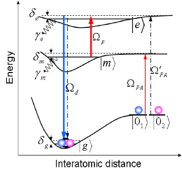
Figure 1: (color online) Schematic diagram: ”$R$-type” transfer in solid arrows comprising the transitons of $\left|0_{1,2}\right\rangle\rightarrow\left|m\right\rangle\rightarrow\left|e\right\rangle\rightarrow\left|g\right\rangle$ with the corresponding coupling fields $\Omega_{PA}$, $\Omega_{p}$ and $\Omega_{d}$, respectively; ”$\Lambda$-type” transfer in dash-dotted arrows with $\left|0_{1,2}\right\rangle\rightarrow\left|e\right\rangle\rightarrow\left|g\right\rangle$ transitions characterized by $\Omega_{PA}^{\prime}$ and $\Omega_{d}$. All the other parameters are described in the text.

Before moving to concrete illustrations of the model, we briefly review the idea of the FR-induced STIRAP method [42, 43]. In a typical FR-induced STIRAP, a number of colliding atoms undergo a strong association into quasi-bound molecules when a magnetic field is swept close to or across the FR, characterized by coupling strength $\alpha$ and binding energy $\varepsilon$. Subsequently, these quasi-bound molecules are further transferred into stable molecules via a STIRAP. Clearly, here $\alpha$ and $\varepsilon$ correspond to $\Omega_{PA}$ and $\delta_{m}$ (see figure 1) in our scheme, respectively. A major advantage of our scheme is that $\Omega_{PA}$ and $\delta_{m}$ can be manipulated more conveniently than $\alpha$ and $\varepsilon$ over the time scales. Because the latter quantities are highly dependent on the atomic intrinsic properties, especially the coupling strength $\alpha$, which is fixed by the hyperfine interaction and is hence independent of time, $\varepsilon$ is experimentally tunable via an external magnetic field, while the former quantities, being controllable by optical means, are easily selected.

Turning to our scheme, as depicted in figure 1, we study a ”$R$-type” five-level atom-polar-molecule formation. Two species of free atoms prepared in $\left|0_{1}\right\rangle$ and $\left|0_{2}\right\rangle$ states are first coupled into molecules in an intermediate high-lying state $\left|m\right\rangle$ with Rabi frequency $\Omega_{PA}$ and detuning $\delta_{m}$. Simultaneously, a pair of pump-dump lasers are applied to move these loosely bound molecules in $\left|m\right\rangle$ down to the lowest molecular ground state $\left|g\right\rangle$, where $\Omega_{p}$, $\Omega_{d}$ stand for coupling strengths and $\delta_{e}$, $\delta_{g}$ for the two- and three-photon detunings. This scheme has several attractive properties. Firstly, the presence of state $\left|m\right\rangle$ brings one extra bound-bound transition from state $\left|m\right\rangle$ to state $\left|e\right\rangle$; hence it becomes easier for the PA field to associate atoms into the $\left|m\right\rangle$, rather than a higher $\left|e\right\rangle$ state. Secondly, transitions $\left|m\right\rangle\rightarrow\left|e\right\rangle$ and $\left|e\right\rangle\rightarrow\left|g\right\rangle$ are preferred because of the favorable bound-bound FCFs. Meanwhile, the $\left|0_{1,2}\right\rangle\rightarrow\left|m\right\rangle$ transition is also accessible by an optimal control of the PA field in the time domain.

As usual, we start our discussions with a set of coupled Gross-Pitaevskii’s equations. In the mean-field treatment, where every quantum field operator $\hat{\Psi}_{i}$ has been replaced by its normalized amplitude $\psi_{i}$ [44], this yields

$$i\dot{\psi}_{0_{1}} =-\frac{\Omega_{PA}}{2}\psi_{0_{2}}^{\ast}\psi_{m},$$ (1)

$$i\dot{\psi}_{0_{2}} =-\frac{\Omega_{PA}}{2}\psi_{0_{1}}^{\ast}\psi_{m},$$ (2)

$$i\dot{\psi}_{m} =-\left(\delta_{m}+i\gamma_{m}\right)\psi_{m}-\frac{\Omega_{PA}}{2}\psi_{0_{1}}\psi_{0_{2}}-\frac{\Omega_{p}}{2}\psi_{e},$$ (3)

$$i\dot{\psi}_{e} =-\left(\delta_{e}+i\gamma_{e}\right)\psi_{e}-\frac{\Omega_{p}}{2}\psi_{m}-\frac{\Omega_{d}}{2}\psi_{g},$$ (4)

$$i\dot{\psi}_{g} =-\delta_{g}\psi_{g}-\frac{\Omega_{d}}{2}\psi_{e},$$ (5)

where $\gamma_{i}$ (i=m,g) is introduced phenomenologically to describe the spontaneous decay of the $\left|i\right\rangle$ state to other undetected states, and it is possible to find a relatively stable $\left|m\right\rangle$ state with its decay rate $\gamma_{m}\ll\gamma_{e}$ [41, 45]. The initial and target states are assumed to be sufficiently stable with $\gamma_{0_{1(2)},g}\equiv 0$. For an easy analysis without loss of the main physics, inter- and intra-species collisions have been ignored under typical parameters [46]. After a global gauge transformation, we can safely consider all the Rabi frequencies to be real positive values without loss of generality.

A CPT state is always expected to move all the population into a target state as long as the adiabatic condition holds. In order to derive the corresponding adiabatic parameter, we first search for the CPT distributions for the following assumptions:

$$\psi_{0_{1,2}}=\phi_{0}e^{-i\mu t},\psi_{e}=0,\psi_{m,g}=\phi_{m,g}e^{-2i\mu t}.$$ (6)

Here $\phi_{i}$ is a steady-state amplitude, we consider $\phi_{0_{1}}=\phi_{0_{2}}=\phi_{0}$ for a balanced system, and $\mu$ is the atomic chemical potential. By ignoring all the decays and inserting equation (6) into equations (1)-(5) with particle number conservation: $2(\phi_{0}^{2}+\phi_{m}^{2}+\phi_{g}^{2})=1$, a generalized three-photon resonance is given by

$$\delta_{g\pm}=-2\mu_{\pm}=\frac{-\Omega_{PA}^{2}/2}{\delta_{m}\pm\sqrt{\delta_{m}^{2}+\Omega_{PA}^{2}\left(3+\chi^{2}\right)/2}},$$ (7)

leading to the following CPT descriptions with $\phi_{e}=0$:

$$\phi_{0} =\sqrt{\frac{1}{2}-\phi_{m}^{2}\left(1+\chi^{2}\right)},$$ (8)

$$\phi_{m} =-\frac{\bar{\Omega}_{PA}/2}{1+\sqrt{1+\bar{\Omega}_{PA}^{2}\left(3+\chi^{2}\right)/2}},$$ (9)

$$\phi_{g} =-\chi\phi_{m}.$$ (10)

where $\bar{\Omega}_{PA}=\Omega_{PA}/\delta_{m}$, $\chi=\Omega_{p}/\Omega_{d}$. In equation (7), the choice of $\delta_{g}$ is determined by $\delta_{m}$. If $\delta_{m}>0$, $\delta_{g}=\delta_{g+}$ and $\mu=\mu_{+}$, whereas if $\delta_{m}<0$, $\delta_{g}=\delta_{g-}$ and $\mu=\mu_{-}$. From equations (8)-(10), we note that when $\left|\bar{\Omega}_{PA}\right|$ and $\chi$ both change from 0 to large positive values, population initially prepared in states $\left|0_{1,2}\right\rangle$ will be gradually converted into molecules in state $\left|g\right\rangle$ under three-photon resonance [equation (7)]. Also it is worth emphasizing that such a CPT state has been perturbed since $\phi_{m}\neq 0$, and is called a ”quasi-CPT” state. In the limit of $\bar{\Omega}_{PA}\ll 1$, population in state $\left|m\right\rangle$ is virtually empty, we find that a complete transfer is still possible as long as $\chi$ varies from 0 to $\infty$. In other words, the change by $\bar{\Omega}_{PA}$ has been accomplished by varying $\Omega_{p}$; thus the existence of state $\left|m\right\rangle$ is quite helpful for a relatively small $\bar{\Omega}_{PA}$ value.

Actually, in the dynamics, if we use a strong PA laser to trigger the $\left|0_{1,2}\right\rangle\rightarrow\left|m\right\rangle$ transition, particle accumulations in state $\left|m\right\rangle$ will inevitably arise. Therefore, in order to avoid a considerable loss from state $\left|m\right\rangle$, pulse durations in STIRAP must be much shorter than $\left|m\right\rangle$ state’s lifetime. On the other hand, if we deeply reduce the $\Omega_{PA}$ value, the population in the $\left|m\right\rangle$ state will greatly be suppressed; meanwhile, a large fraction of atoms are left in the continuum, unpaired, because of a poor atom-molecule coupling strength. This conflict can be generalized to the properties of a quasi-CPT state, in which case one may prefer the use of moderate PA power.

Results in equations (8)-(10) are for the case of $\delta_{m}\neq 0$. If $\delta_{m}=0$, i.e. the PA laser is exactly resonant with the free-bound transition, then equation (7) is reduced to $\delta_{g\pm}=\pm\Omega_{PA}/(6+2\chi^{2})^{1/2}$ with the following CPT solutions:

$$\phi_{0}^{2}=2\phi_{m}^{2}=2\phi_{g}^{2}/\chi^{2}=\left(3+\chi^{2}\right)^{-1}.$$ (11)

Equation (11) shows a constant population ratio between states $\left|0_{1,2}\right\rangle$ and $\left|m\right\rangle$, i.e. $\phi_{0}^{2}/\phi_{m}^{2}=2$. This equality contrasts with the standard CPT evolution, especially at t=0, which implies a poor transfer efficiency at $\delta_{m}=0$. As a result, a nonzero $\delta_{m}$ value is favored in our consideration.

3 Adiabatic Theorem

To derive the adiabatic parameter for the quasi-CPT state, we adopt a standard linearized approach as in [47, 48] by adding a small fluctuation $\delta\psi_{i}$ to the instantaneous steady-state solution $\phi_{i}$,

$$\psi_{0_{1,2}}=\left(\phi_{0}+\delta\psi_{0_{1,2}}\right)q\left(t\right),\psi_{e}=\delta\psi_{e}q^{2}\left(t\right),\psi_{m,g}=\left(\phi_{m,g}+\delta\psi_{m,g}\right)q^{2}\left(t\right)$$ (12)

where $q\left(t\right)=\exp[-\int_{0}^{t}\mu\left(t^{\prime}\right)dt^{\prime}]$, and $\mu(t)$ is a time-dependent chemical potential given by $\mu\left(t\right)=\mu_{+\left(-\right)}$ (see equation (7)). Substituting equation (12) into the mean-field equations (1)-(5) with the help of CPT descriptions, we eventually arrive at a set of linearized equations for the vector $\mathbf{\delta}\mathbf{\psi=}\left[\delta\psi_{0_{1}},\delta\psi_{0_{2}},\delta\psi_{m},\delta\psi_{e},\delta\psi_{g}\right]^{T}$ with its conjugate vector $\mathbf{\delta}\mathbf{\psi}^{\ast}$

$$\mathbf{\delta\dot{\Psi}=-}i\mathbf{M\delta\Psi-\Gamma\delta\Psi-\dot{\Phi}},$$ (13)

where

$$\mathbf{M=}\left(\begin{array}[c]{cc}\mathbf{A}&\mathbf{B}\\ -\mathbf{B}&-\mathbf{A}\end{array}\right),\mathbf{\Gamma=}\left(\begin{array}[c]{cc}\mathbf{\gamma}&0\\ 0&\mathbf{\gamma}\end{array}\right),$$

and

$$\mathbf{A} =-\frac{1}{2}\left(\begin{array}[c]{ccccc}2\mu&0&\Omega_{PA}\phi_{0}&0&0\\ 0&2\mu&\Omega_{PA}\phi_{0}&0&0\\ \Omega_{PA}\phi_{0}&\Omega_{PA}\phi_{0}&2\left(\delta_{m}+2\mu\right)&\Omega_{p}&0\\ 0&0&\Omega_{p}&0&\Omega_{d}\\ 0&0&0&\Omega_{d}&0\end{array}\right),$$ (19)

$$\mathbf{B} =-\frac{\Omega_{PA}\phi_{m}}{2}\left(\begin{array}[c]{ccccc}0&1&0&0&0\\ 1&0&0&0&0\\ 0&0&0&0&0\\ 0&0&0&0&0\\ 0&0&0&0&0\end{array}\right).$$ (25)

In equation (13), some notations are $\mathbf{\delta\Psi=}\left[\mathbf{\delta}\mathbf{\psi,\delta}\mathbf{\psi}^{\ast}\right]^{T}$, $\mathbf{\dot{\Phi}=}\left[\mathbf{\dot{\phi},\dot{\phi}}\right]^{T}$ with $\mathbf{\dot{\phi}=}\left[\dot{\phi}_{0},\dot{\phi}_{0},\gamma_{m}\phi_{m}+\dot{\phi}_{m},0,\dot{\phi}_{g}\right]^{T}$. $\mathbf{\gamma}$ is a $5\times 5$ matrix with $\gamma_{33}=\gamma_{m}$ and $\gamma_{44}=\gamma_{e}$ being the only nonzero elements. In addition, we have assumed detunings $\delta_{e,g}=-2\mu(t)$ to be chirped [49].

Furthermore, we introduce a generalized Bogoliubov-de Gennes (BdG) equation for matrix $\mathbf{M}$,

$$\mathbf{M}\left(t\right)\mathbf{w}_{i}\left(t\right)=\omega_{i}\left(t\right)\mathbf{w}_{i}\left(t\right),$$ (26)

where $\omega_{i}$ and $\mathbf{w}_{i}=\left[\mathbf{u}_{i},\mathbf{v}_{i}\right]^{T}$ are the well-defined $i$th eigenenergy and eigenvector, respectively. $\mathbf{u}_{i}$ and $\mathbf{v}_{i}$ contain familiar Bogoliubov $u$-$v$ parameters for each species

$$\mathbf{u}\left(\mathbf{v}\right)_{i}=[u\left(v\right)_{i0_{1}},u\left(v\right)_{i0_{2}},u\left(v\right)_{im},u\left(v\right)_{ie},u\left(v\right)_{ig}]^{T}.$$ (27)

From the BdG equation, taking into account the special structure of matrix M, one can show the quantities $\omega_{i}^{2}$ are the eigenenergies of the matrix $(\mathbf{A}+\mathbf{B})(\mathbf{A}-\mathbf{B})$, which can be obtained from the following equation:

$$\left(\omega_{i}^{2}\right)^{2}\left(\left(\omega_{i}^{2}\right)^{3}-a_{1}\left(\omega_{i}^{2}\right)^{2}+a_{2}\left(\omega_{i}^{2}\right)-a_{3}\right)=0,$$ (28)

where the coefficients $a_{i}$ are given as

$$a_{1} =\left(\delta_{m}+2\mu\right)\left(\delta_{m}+6\mu\right)+\frac{\Omega_{p}^{2}+\Omega_{d}^{2}}{2},$$ (29)

$$a_{2} =\frac{\left(\delta_{m}+2\mu\right)}{2}\left(2\Omega_{p}^{2}\mu+\Omega_{d}^{2}\left(\delta_{m}+6\mu\right)\right)+\frac{\left(\Omega_{p}^{2}+\Omega_{d}^{2}\right)^{2}}{16},$$ (30)

$$a_{3} =\frac{\left(\delta_{m}+2\mu\right)\Omega_{d}^{2}}{16}\left(4\Omega_{p}^{2}\mu+\Omega_{d}^{2}\left(\delta_{m}+6\mu\right)\right).$$ (31)

Eigenenergies implied in equation (28) comprise a doublet 0 mode $\omega_{0,1}=0$ and three pairs of excited modes $\left(\omega_{j},-\omega_{j}^{\ast}\right)$ (j=2,3,4). We find that $\omega_{j}$ is real and has to be determined by biorthonormal relations for its corresponding eigenvector $\mathbf{w}_{j}$. Detailed elucidations of biorthonormality have been published elsewhere [50]. In addition, we realize that the dynamical instability is impossible here due to the absence of collisions.

To accomplish the goal of deriving the adiabatic theorem, we have to expand an arbitrary vector $\mathbf{\delta\Psi}$ in the dressed-state picture with a complete set of eigenvectors. By solving the BdG equation with 0 eigenenergies, we are able to obtain $\mathbf{w}_{0}$ and $\mathbf{w}_{1}$ (unnormalized) explicitly using Gram-Schmidt orthogonalization,

$$\mathbf{w}_{0} =\left(-1,1,0,0,0,1,-1,0,0,0\right)^{T},$$ (32)

$$\mathbf{w}_{1} =\left(\frac{\phi_{0}}{2\phi_{m}},\frac{\phi_{0}}{2\phi_{m}},1,0,-\chi,\frac{-\phi_{0}}{2\phi_{m}},\frac{-\phi_{0}}{2\phi_{m}},-1,0,\chi\right)^{T}.$$ (33)

Here $\mathbf{w}_{0}$, being a real dark state, is entirely decoupled with other eigenmodes, because its source term ($\mathbf{w}_{0}^{T}\mathbf{\dot{\Phi}}$) and inter-coupling term ($\mathbf{w}_{0}^{T}\mathbf{\Gamma\mathbf{\eta}_{+}w}_{j}$) both vanish (see equation (38) below for detailed notations), whereas, $\mathbf{w}_{1}$ is most likely to be triggered through its nonzero inter-coupling strength ($\mathbf{w}_{1}^{T}\mathbf{\Gamma\mathbf{\eta}_{+}w}_{j}$), which can be roughly estimated by its decay rate

$$\mathbf{w}_{1}^{T}\mathbf{\Gamma\eta}_{+}\mathbf{Q}=\frac{\gamma_{m}}{\phi_{0}^{2}/2\phi_{m}^{2}+2(1+\chi^{2})}\equiv 1/\tau_{cpt},$$ (34)

where $\mathbf{Q}$ is a newly introduced vector complementary to $\mathbf{w}_{1}$ with a well-defined normalization,

$$\mathbf{w}_{1}^{T}\mathbf{\eta}_{+}\mathbf{Q}=1,$$ (35)

through the definition of

$$\mathbf{MQ=w}_{1}/v.$$ (36)

Here, $v$ is a coefficient to be determined, and $\mathbf{\eta}_{+}$(and $\mathbf{\eta}_{-}$ below) are given in [50]. Combining equation (35) with (36), we find the vector $\mathbf{Q}$ takes a special form: $\mathbf{Q}=\mathbf{[}q_{0},q_{0},q_{m},q_{e},q_{g},q_{0},q_{0},q_{m},q_{e},q_{g}\mathbf{]}^{T}$. Detailed expressions for $q_{i}$ and $v$ are presented in the appendix.

The CPT lifetime $\tau_{cpt}$ defined in equation (34) is clearly inversely-proportional to $\gamma_{m}$ and $\phi_{m}$, which agrees with our intuitions. In other words, the presence of state $\left|m\right\rangle$ actually gives rise to a finite lifetime for the quasi-CPT state. Any pulse duration used in the system has to be much shorter than $\tau_{cpt}$; otherwise, a big particle loss from state $\left|m\right\rangle$ is unavoidable. One effective way to achieve a long $\tau_{cpt}$ is to search for a relatively stable $\left|m\right\rangle$ state with a small $\gamma_{m}$ value. Other excited eigenenergies and eigenvectors are too complicated to list here, but they can be conveniently derived from equation (26) with (28).

Since other inter-coupling strengths for $\mathbf{w}_{1}$ are also proportional to $\gamma_{m}$ as in equation (34) and $\gamma_{m}$ is considered to be much smaller than $\gamma_{e}$, we shall safely ignore the contributions from $\mathbf{w}_{1}$ and expand $\mathbf{\delta\Psi}$ in the parameter space with the help of three excited eigenmodes $\mathbf{w}_{j}$ (j=2,3,4) only, taking the form of

$$\mathbf{\delta\Psi=}\sum_{j=2}^{4}\left(c_{j}\mathbf{\eta}_{+}\mathbf{w}_{j}-c_{j}^{\ast}\mathbf{\eta}_{-}\mathbf{w}_{j}^{\ast}\right).$$ (37)

Through inserting equation (37) into (13), and with the help of biorthonormality relations, finally, we obtain a set of coupling equations for $c_{j}\left(t\right)$,

$$\dot{c}_{j}+i\omega_{j}c_{j}+\mathbf{\mathbf{w}}_{j}^{T}\mathbf{\Gamma\delta\Psi}=\mathbf{-\mathbf{w}}_{j}^{T}\mathbf{\dot{\Phi}}$$ (38)

Terms like $\mathbf{\dot{w}}_{j}^{T}\mathbf{\delta\Psi}$ have been eliminated in equation (38) because the eigenvector $\mathbf{\mathbf{w}}_{j}$ changes very slowly in the adiabatic limit. Generally speaking, if a system is said to operate in an adiabatic regime, population in any excited mode (nonzero eigen-mode) remains small. Hence, we shall introduce a typical adiabatic parameter definition

$$r\left(t\right)=\sqrt{\frac{\left|c_{2}\right|^{2}+\left|c_{3}\right|^{2}+\left|c_{4}\right|^{2}}{3}}\ll 1$$ (39)

A reduction in the $r$-value means an increase in the adiabaticity; in general, it can be accomplished by a longer pulse or a stronger pump field. In the adiabatic regime, if a system evolves in a CPT state, an entire population conversion is achievable. However, the CPT lifetime implied in our model places a limitation for both the pulse duration and PA intensity, leading to a slightly larger $r$-value. This point will be discussed in section 4.1 toward the goal of obtaining an optimal pulse duration and PA intensity for an efficient transfer.

In equation (38), since $\dot{c}_{j}$ can be ignored adiabatically, we further rewrite it as a series of linearized coupling equations:

$$\left(\begin{array}[c]{cc}\mathbf{F}+i\mathbf{\omega}&\mathbf{G}\\ \mathbf{G}&\mathbf{F}-i\mathbf{\omega}\end{array}\right)\left(\begin{array}[c]{c}\mathbf{c}\\ \mathbf{c}^{\ast}\end{array}\right)=-\left(\begin{array}[c]{c}\dot{\Phi}_{w}\\ \dot{\Phi}_{w}\end{array}\right)$$ (40)

where

$$\mathbf{F=}\left(\begin{array}[c]{ccc}f_{22}&f_{23}&f_{24}\\ f_{23}&f_{33}&f_{34}\\ f_{24}&f_{34}&f_{44}\end{array}\right),\mathbf{G=}\left(\begin{array}[c]{ccc}0&g_{23}&g_{24}\\ -g_{23}&0&g_{34}\\ -g_{24}&-g_{34}&0\end{array}\right),$$

with the definitions of $\mathbf{c=}\left[c_{2},c_{3},c_{4}\right]^{T}$, $\dot{\Phi}_{w}=[\mathbf{\mathbf{w}}_{2}^{T}\mathbf{\dot{\Phi},\mathbf{w}}_{3}^{T}\mathbf{\dot{\Phi},\mathbf{w}}_{4}^{T}\mathbf{\dot{\Phi}]}^{T}$, $\mathbf{\omega}=\omega_{j}\mathbf{D}$ (j=2,3,4), $\mathbf{D}$ is a $3\times 3$ unit matrix, and

$$f_{ij} =\gamma_{m}\left(u_{im}u_{jm}-v_{im}v_{jm}\right)+\gamma_{e}\left(u_{ie}u_{je}-v_{ie}v_{je}\right),$$ (41)

$$g_{ij} =\gamma_{m}\left(v_{im}u_{jm}-u_{im}v_{jm}\right)+\gamma_{e}\left(v_{ie}u_{je}-u_{ie}v_{je}\right),$$ (42)

We solve $c_{j}(c_{j}^{\ast})$ values from equations (40) numerically and insert them into equation (39), a time-dependent $r$-function is ultimately accessible. It needs to be noted that all the $u(v)$s in equation (41) and (42) have been normalized according to biorthogonality,

$$\mathbf{w}_{i}^{T}\mathbf{\eta}_{+}\mathbf{w}_{j}=\delta_{ij},\mathbf{w}_{i}^{T}\mathbf{\eta}_{-}\mathbf{w}_{j}=0.$$ (43)

4 Numerical Analysis

In the following numerical calculations, we intended to achieve a highly-efficient ground molecular production under an optimization of all the optical fields, including $\Omega_{PA},$ $\Omega_{p}$ and $\Omega_{d}$. From CPT descriptions [equations (8-10)], we adopt a common pair of counterintuitive pump-dump pulses for $\left|m\right\rangle$-$\left|g\right\rangle$ transition with the same width $T$

$$\Omega_{p,d}=\frac{\Omega_{p,d}^{0}}{2}\left(1\pm\tanh\left(\frac{t-t_{p,d}}{T}\right)\right)$$ (44)

where $\Omega_{p,d}^{0}$, $t_{p,d}$ are for the peak Rabi frequencies and central positions respectively. Based on equations (8)-(10), the PA Rabi frequency $\Omega_{PA}$, which must start from 0, is considered to share the same profile as $\Omega_{p}$ except for a different peak amplitude $\Omega_{PA}^{0}$. Here, the detuning $\delta_{m}$ is fixed at a finite value for simplicity.

4.1 Optimal PA pulse

In what follows, we seek to gain from the $r$-value in equation (39) insights into the parameters, especially for an appropriate PA amplitude $\Omega_{PA}^{0}$ and a pulse duration $T$. As we already understand, applying a longer pulse or a more intense PA laser will lead to a lower $r$-value. If a system’s adiabaticity ($r$-value) is kept in a low level, which means the system will operate within the adiabatic regime, any excited modes are greatly suppressed. In a pure-CPT environment, adiabaticity indeed becomes a sufficient criterion for a complete transfer. However, in our scheme, we observe in addition to adiabaticity, a long CPT lifetime is another significant criterion for an efficient transfer.

In a dynamical process, the $r$-value obtained from equation (39) varies with time. We find that $r$-value estimated at $t_{s}$ which is defined by $\phi_{0}^{2}(t_{s})=2\phi_{g}^{2}(t_{s})$ turns out to be a good estimate of the degree of adiabaticity. Thus, $r_{s}$ and $\tau_{cpt}$ values displayed in figure 2(a), (b) are both evaluated at $t=t_{s}$.

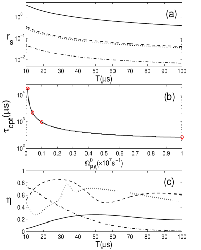
Figure 2: (a) $r$-value at $t=t_{s}$ versus pulse duration $T$ under different PA amplitudes: from top to bottom $\Omega_{PA}^{0}=10^{5}$ s^-1, $4\times 10^{5}$ s^-1, $10^{6}$ s^-1 and $10^{7}$ s^-1, respectively. (b) $\tau_{cpt}$ estimated at $t=t_{s}$ as a function of $\Omega_{PA}^{0}$. The four circles (from left to right) denote $\tau_{cpt}$=17.8 ms, 2.2 ms, 0.97 ms, 257 $\mu s$ with respect to the corresponding $\Omega_{PA}^{0}$s shown in (a). (c) Final molecular production $\eta=2|\psi_{g}(\infty)|^{2}$ versus pulse duration $T$ under the same four cases as in (a). The other parameters are described in the text.

Figure 2(a) and (c) present the variations of adiabaticity $r(t_{s})$ and final efficiency $\eta$(=$\left|2\psi_{g}(\infty)\right|^{2}$) as a function of pulse width $T$, respectively. As plotted in figure 2(a), either a longer pulse (from left to right) or a stronger PA amplitude (from the top to the bottom) leads to an improved adiabaticity. Furthermore, when $\Omega_{PA}^{0}$ is very weak, such as 10⁵ s^-1 (in solid), the $r$-value is around 1.0, which cannot well satisfy the adiabatic condition $r\ll 1$. Although at this time, the CPT lifetime in figure 2(b) is long enough (more than 15 ms) to support a longer pulse duration, a large part of atoms will be left in the continuum, resulting in poor molecular production, which is no more than 30% (see the solid curve in (c)). On the other hand, if we use an intense laser, $\Omega_{PA}^{0}=10^{7}$ s^-1, then the adiabaticity reduces into the 0.01 level, whereas simultaneously, the CPT lifetime is only around 250$\mu s$, leading to a dramatic reduction in $\eta$ as $T$ increases (see the dash-dotted curve in figure 2(c)), because with a longer $T$ value, a number of molecules decay spontaneously due to $\gamma_{m}$. Obviously, if $T<20\mu s$, a relatively higher $\eta$ value ($>$50%) is still attainable.

In addition, we study two moderate cases with the PA amplitudes: $\Omega_{PA}^{0}=4\times 10^{5}$ s^-1 (in dashed) and $\Omega_{PA}^{0}=10^{6}$ s^-1 (in dotted). No impressive differences are observable in adiabaticity according to figure 2(a), where both are around the 0.1 level. Meanwhile, the $\tau_{cpt}$ values represented in figure 2(b) are both close to 1 ms, which do offer more space for a tunable $T$ value. Final efficiencies in figure 2(c) clearly exhibit a $T$-dependent feature, while staying at a highly efficient level compared with two former cases.

In light of the above discussions, we conclude that the adiabaticity indeed serves as a useful tool to select favorable parameters. Meanwhile, it is equivalently important to take the CPT lifetime into consideration. Here, we prefer to use $T=30$ $\mu s$, $\Omega_{PA}^{0}=4\times 10^{5}$ s^-1.

4.2 Optimal pump-dump pulse sequence

The goal of this subsection is to design the optimal pump-dump two-pulse sequence to maximize the yield of molecules. Clearly, there are five individual parameters to be determined: $t_{p}$, $t_{d}$, $\Omega_{p}^{0}$, $\Omega_{d}^{0}$ and $\delta_{m}$. Such a five-parameter variation is difficult to carry out. However, from the CPT descriptions, we guess that the population dynamics are most likely to be affected by the ratio $\chi=\Omega_{p}/\Omega_{d}$ instead of the $\Omega_{p}$ and $\Omega_{d}$ values. Therefore, we introduce two new variables, which are $dt=t_{d}-t_{p}$ for pulse delay and $\chi^{0}=\Omega_{p}^{0}/\Omega_{d}^{0}$ for peak amplitude ratio. In combination with the one-photon detuning $\delta_{m}$, there are three effective quantities to be optimized.

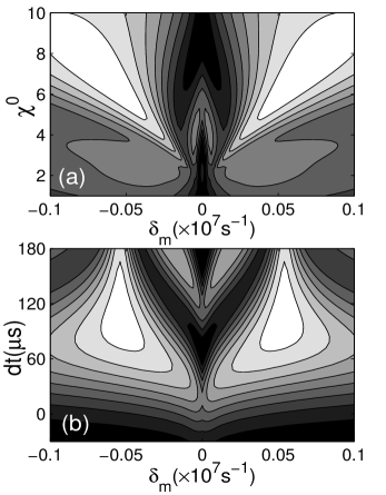
Figure 3: Contour plot of final transfer efficiencies under different sets of (a) $\left[\delta_{m},\chi^{0}\right]$ where $dt=105\mu s$ and (b) $\left[\delta_{m},dt\right]$, where $\chi^{0}=6$. Here, $\Omega_{d}^{0}=10^{7}$ s^-1, $t_{p}=75$ $\mu s$. Lighter areas correspond to high efficiencies. Pure white areas denote efficiencies more than $80\%$. The other parameters are listed in the text.

Figure 3(a) and (b) show the contour plots of the final molecular productions for sets of $\left[\delta_{m},\chi^{0}\right]$ and $\left[\delta_{m},dt\right]$, respectively, where the lighter areas correspond to higher efficiencies. Especially, pure white regimes are for $\eta\geq 80\%$. These two mappings have several attractive features. Firstly, a symmetric pattern along the $\delta_{m}$ direction is explicitly observable, which can be ascribed to the existence of a three-photon resonance [equation (7)]. Regardless of whether $\delta_{m}$ is positive or negative, either $\delta_{g+}=-2\mu_{+}$ or $\delta_{g-}=-2\mu_{-}$ will be satisfied. In other words, a double-resonant condition must hold on both sides of $\delta_{m}$, leading to a symmetric double-peak pattern. Similar patterns have been demonstrated by the Autler-Townes splitting effect [51, 52], which usually takes place when an optical field is detuned close to an exact transition frequency. To be more understandable, if we artificially add a small perturbation to a resonance, the double-peak profile will be correspondingly shifted. Since this shift employs no improvement in the molecule production, we will leave this point for future interested readers.

Secondly, if we fix $\left|\delta_{m}\right|$ around $0.05\times 10^{7}$ s^-1 and gradually increase the values of $\chi^{0}$ and $dt$, the final transfer efficiencies express similar variations. Seen in figure 3(a), based on $\Omega_{d}^{0}=10^{7}$s^-1, $dt=105\mu s$, if $\chi^{0}$ changes from 1.0 to 6.0, a dramatic enhancement for $\eta$ is explicit. When further increasing $\chi^{0}$ up to 10.0, $\eta$ values will be slowly decreasing. A similar trend with $\eta$ as the pulse delay $dt$ varies is depicted in figure 3(b) where $\chi^{0}=6$, $\Omega_{d}^{0}=10^{7}$s^-1. When $\delta_{m}=0$, efficiencies are very poor, which agrees with our CPT predictions equation (11) in section 2. Finally, we find that the base value of $\Omega_{d}^{0}$ offers few contributions to the transfer. If $\Omega_{d}^{0}$ is set as $2\times 10^{7}$s^-1, we will obtain a much analogous contour plot to figure 3(a)(not shown).

A brief conclusion for the sections 4.1 and 4.2 is that we are provided with rich ways to select relevant parameters for optimal atom-molecule conversion.

4.3 Population dynamics

In the following, we consider a concrete example in our ”$R$-type” scheme using the parameters based on our previous discussions. Optimal parameters are given by $T=30$ $\mu s$, $\Omega_{PA}^{0}=4\times 10^{5}$ s^-1, $\Omega_{p}^{0}=6\times 10^{7}$ s^-1, $\Omega_{d}^{0}=10^{7}$ s^-1, $t_{p}=75$ $\mu s$, $t_{d}=180$ $\mu s$, $\left|\delta_{m}\right|=5.4\times 10^{5}$ s^-1, $\gamma_{m}=3\times 10^{4}$ s^-1 and $\gamma_{e}=10^{7}$ s^-1. Numerical results are plotted in figure 4. By directly integrating the mean-field dynamic equations (1)-(5), we produce a population dynamics which contains all the field amplitudes in figure 4(b). Observably, more than 85% of the atoms $\psi_{0_{1,2}}^{2}$ convert into ground-state molecules $\psi_{g}^{2}$. Compared with the CPT dynamics shown in figure 4(a), a good agreement is clearly seen, except for a slightly lower $2\psi_{g}^{2}$ coming from spontaneous decays. In particular, we need to mention that the $\phi_{m}^{2}(\psi_{m}^{2})$ amplitude (dotted) has been deeply suppressed, with a maximum value smaller than 0.02.

Figure 4(c) represents the adiabaticity defined in equation (39) as time changes (in solid). By solving equations (40) numerically, a complete $r$-value is able to be determined from the $c_{j}$ values. Three excited eigenenergies obtained from equation (28) are displayed in figure 4(d) and the inset, where $\omega_{3}$ is smaller than $\omega_{2,4}$ by orders of magnitude. In the dressed state picture, $\omega_{j}$ stands for the energy of the $j$th eigenstate, and generally speaking, a higher-energy eigenstate is usually more difficult to populate than a lower one. Thereby, in deriving the adiabaticity, we shall safely neglect the contributions from $\omega_{2,4}$ and $\mathbf{w}_{2,4}$, simplifying equations (40) with $\omega_{3},\mathbf{w}_{3}$ only, yielding

$$i\omega_{3}c_{3}+f_{33}c_{3}=-\mathbf{\mathbf{w}}_{3}^{T}\mathbf{\dot{\Phi}},$$ (45)

which leads to a reduced assessment on adiabaticity: $r_{a}=\left|\mathbf{\mathbf{w}}_{3}^{T}\mathbf{\dot{\Phi}/(}i\omega_{3}+f_{33})\right|/\sqrt{3}$. Clearly, $r_{a}$ matches with $r$ in figure 4(c) perfectly.

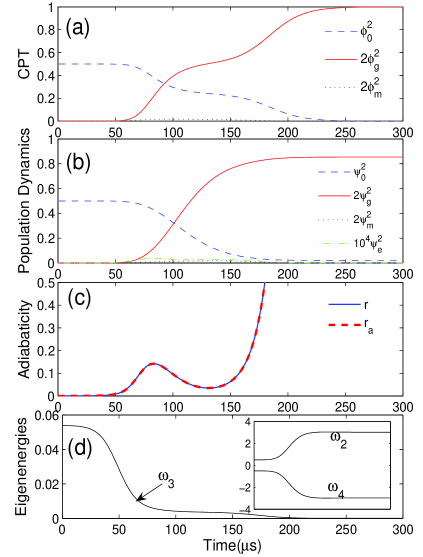
Figure 4: (color online) (a) CPT dynamics, (b) population dynamics, (c) time-dependent adiabaticity values, (d) three excited eigen-energies as time changes where $\omega_{3}$ is at least two orders smaller than $\omega_{2,4}$ (shown in the inset).

One critical concern in our scheme is the stability of state $\left|m\right\rangle$, which indeed plays a vital role in determining the final transfer efficiency. In our calculations, we use the $\left|m\right\rangle$ state lifetime to be $\tau_{m}=1/(2\pi\gamma_{m})=5.3\mu s$, which is comparable with the earlier work of Napolitano et al [45]. Figure 5 displays how the final efficiency $\eta$(=2$\psi_{g}^{2}(\infty)$) varies as a function of $\tau_{m}$. Clearly, if $\tau_{m}$ is smaller than $1\mu s$, $\eta$ drops rapidly as $\tau_{m}$ becomes shorter. However, if we are able to find a more stable intermediate state, with a lifetime longer than 10 $\mu s$, the corresponding transfer efficiency reaches as high as 90%. The arrow shown in figure 5 points to the $\tau_{m}$ value used in our paper.

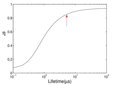
Figure 5: The final transfer efficiency $\eta$ as a function of the intermediate state lifetime $\tau_{m}$. An arrow corresponds to the lifetime we have used.

Finally, it is meaningful for a numeric estimate of the feasibility of our scheme by taking the KRb molecule as a possible candidate in experiment. Based on the predictions in [24, 53], it is experimentally possible to find out an appropriate $\left|m\right\rangle$ state with a relative long lifetime, e.g. $3^{1}\Sigma^{+}$. There is a transition dipole moment of $\sim$ 1 ea₀ for the state $3^{1}\Sigma^{+}$, which corresponds to the lifetime of several $\mu s$. In addition, the $1^{1}\Pi$ is a good candidate for the high-lying $\left|e\right\rangle$ state because of its purely singlet character and favorable transition dipole moment associated with the lowest singlet state $1^{1}\Sigma^{+}$ ($\left|g\right\rangle$ state). A rough estimation of the PA power, adopting the parameters of the free-bound FCF $I_{FCF}\sim$10^-14 m^3/2 for KRb [54]-[56] and an initial atomic density $n_{0}=10^{20}$m^-3, gives rise to a PA laser intensity of $I_{PA}=2c\varepsilon_{0}(\hbar\Omega_{PA}^{0(el)}/\mu)^{2}\approx 512.7$ W/cm² for our ”R-type” scheme, where $c$ is the light velocity, $\varepsilon_{0}$ is vacuum permittivity, $\mu$ is the dipole moment, $\Omega_{PA}^{0(el)}$ is the electronic Rabi frequency defined by $\Omega_{PA}^{0(el)}=\Omega_{PA}^{(0)}/(I_{FCF}\sqrt{n_{0}})$ [54]. However, in a standard ”$\Lambda$-type” system (see figure 1), the absence of state $\left|m\right\rangle$ requires a more intense PA field to stimulate particles into the highly excited state $\left|e\right\rangle$. As a result, to achieve the same production rate of molecules as in our ”R-type” case, the required PA power must be $\Omega_{PA}^{\prime 0}\sim 6.4\times 10^{6}$ s^-1. The corresponding PA intensity is $I_{PA}^{\prime}\sim 1.31\times 10^{5}$ W/cm², giving other parameters the same as in the ”R-type” case. Evidently, the above numeric estimate shows a more than 250 times power reduction in our ”R-type” approach.

5 Summary

Although the magnetic FR-assisted PA technique has been considered as the most promising way for the purpose of overcoming the PA weakness, the primary drawback in such a scheme is the strong inelastic-collisional loss of Feshbach molecules, especially when the magnetic field is tuned near the resonant point. To eliminate the bottleneck in the magnetic FR-assisted PA technique, we work out a robust all-optical atom-molecule conversion model through a ”$R$-type” photoassociative STIRAP, where an intermediate state $\left|m\right\rangle$ is introduced to form a quasi-CPT state. In terms of the detailed adiabatic theorem, we show that the quasi-CPT state can lead to a higher atom-molecule transfer efficiency with a lower PA laser power, compared to the normal CPT state in the conventional all-optical ”$\Lambda$-type” two-color PA configuration.

The key reason for the lowered power of PA laser is due to the existence of an intermediate state $\left|m\right\rangle$. In this case, it is easier to photoassociate free atoms into this low-lying $\left|m\right\rangle$ state, rather than a high-lying $\left|e\right\rangle$ state. Since molecules in state $\left|m\right\rangle$ are unstable, the subsequent STIRAP transfer from the intermediate state $\left|m\right\rangle$ to the final state $\left|g\right\rangle$ must be rapid enough to avoid the loss of molecules from the $\left|m\right\rangle$ state, here characterized by a finite CPT lifetime. In addition, we also show that the lifetime of state $\left|m\right\rangle$ will significantly affect the final transfer efficiency. A specific estimation to illustrate the feasibility of our approach is performed. Finally we want to emphasize that the scheme proposed here is the first one to overcome the inefficiency of PA with only all-optical fields involved. This may open up new opportunities for experimental endeavors to create polar molecular condensates directly from ultracold atoms. A more careful treatment taking into account nonlinear collisions will be left for future explorations.

Appendix A $\mathbf{Q}$ vector

$q_{i}$ values in vector $\mathbf{Q}$ are given by

$$q_{0} =-\frac{\phi_{0}^{2}+2\phi_{m}^{2}\left(1+\chi^{2}\right)}{2v\Omega_{PA}\phi_{0}\phi_{m}^{2}}$$ (46)

$$q_{m} =-\frac{1}{v\Omega_{PA}\phi_{m}}$$ (47)

$$q_{e} =\frac{2\chi}{v\Omega_{d}}$$ (48)

$$q_{g} =\frac{\chi}{v\Omega_{PA}\phi_{m}}$$ (49)

and

$$v=-\frac{\phi_{0}^{2}+4\phi_{m}^{2}(1+\chi^{2})}{\Omega_{PA}\phi_{m}^{3}}$$ (50)

References

References

- [1] Doyle J, Friedrich B, Krems R V and Masnou-Seeuws F, 2004 Eur. Phys. J. D 31, 149
- [2] Carr L D, DeMille D, Krems R V and Ye J 2009 New J. Phys. 11, 055049
- [3] Santos L, Shlyapnikov G V, Zoller P, and Lewenstein M 2000 Phys. Rev. Lett. 85, 1791
- [4] Yi S and You L 2000 Phys. Rev. A. 61, 041604(R)
- [5] DeMille D 2002 Phys. Rev. Lett. 88, 067901
- [6] André A et al. 2006 Nat. Phys. 2, 636
- [7] Yelin S F, Kirby K and Côté R 2006 Phys. Rev. A. 74, 050301(R)
- [8] Kozlov M G and Labzowsky L N 1995 J. Phy. B, 28, 1933
- [9] DeMille D et al. 2000 Phys. Rev. A. 61, 052507
- [10] Hudson J J, Sauer B E, Tarbutt M R, and Hinds E A 2002 Phys. Rev. Lett. 89, 023003
- [11] Hudson E R, Lewandowski H J, Sawyer B C, and Ye J, 2006 Phys. Rev. Lett. 96, 143004
- [12] Flambaum V V and Kozlov M G 2007 Phys. Rev. Lett. 99, 150801
- [13] DeMille D et al. 2008 Phys. Rev. Lett. 100, 023003
- [14] Weinstein J D et al. 1998 Nature 395, 148
- [15] Jones K M, Tiesinga E, Lett P D and Julienne P S 2006 Rev. Mod. Phys, 78, 483
- [16] Köhler T, Góral K and Julienne P S 2006 Rev. Mod. Phys, 78, 1311
- [17] Bergmann K, Theuer H, and Shore B W, 1998 Rev. Mod. Phys, 70, 1003
- [18] Winkler K et al. 2007 Phys. Rev. Lett. 98, 043201
- [19] Lang F et al. 2008 Phys. Rev. Lett. 101, 133005
- [20] Ospelkaus S et al. 2008 Nat. Phys. 4 622
- [21] Ni K-K et al. 2008 Science, 322, 231
- [22] Ospelkaus S et al. 2009 Faraday Discuss., 142, 351
- [23] Danzl J G et al. 2008 Science, 321, 1062
- [24] Aikawa K, Akamatsu D, Kobayashi J, Ueda M, Kishimoto T and Inouye S 2009 New J. Phys. 11, 055035
- [25] Wynar R, Freeland R S, Han D J, Ryu C and Heinzen D J 2000 Science, 287, 1016
- [26] Tolra B L, Drag C, and Pillet P 2001 Phys. Rev. A. 64, 061401(R)
- [27] Sage J M, Sainis S, Bergeman T, and DeMille D 2005 Phys. Rev. Lett. 94, 203001
- [28] Kerman A J, Sage J M, Sainis S, Bergeman T, and DeMille D 2004 Phys. Rev. Lett. 92, 033004
- [29] Viteau M 2008 Science, 321, 232
- [30] Deiglmayr J et al. 2008 Phys. Rev. Lett. 101, 133004
- [31] Vardi A, Abrashkevich D, Frishman E, and Shapiro M 1997 J. Chem. Phys. 107, 6166
- [32] Vardi A, Shapiro M and Bergmann K, 1998 Opt. Express. 4, 91
- [33] van Abeelen F A, Heinzen D J and Verhaar B J 1998 Phys. Rev. A. 57, r4102
- [34] Courteille Ph, Freeland R S, Heinzen D J, van Abeelen F A and Verhaar B J 1998 Phys. Rev. Lett. 81, 69
- [35] Tolra B L et al. 2003 Europhy. Lett. 64, 171
- [36] Junker M et al. 2008 Phys. Rev. Lett. 101, 060406
- [37] Deiglmayr J et al. 2009 New J. Phys, 11, 055034
- [38] Pellegrini P, Gacesa M, and Côté R 2008 Phys. Rev. Lett. 101, 053201
- [39] Kuznetsova E, Gacesa M, Pellegrini P, Yelin S F and Côté R 2009 New J. Phys, 11, 055028
- [40] Nikolov A N, Ensher J R, Eyler E E, Wang H, Stwalley W C and Gould P L 2000 Phys. Rev. Lett. 84, 246
- [41] Band Y B and Julienne P S 1995 Phys. Rev. A. 51, R4317
- [42] Kokkelmans S J J M F, Vissers H M J and Verhaar B J 2001 Phys. Rev. A. 63, 031601
- [43] Mackie M 2002 Phys. Rev. A. 66, 043613
- [44] Heinzen D J, Wynar R, Drummond P D and Kheruntsyan K V 2000 Phys. Rev. Lett. 84, 5029
- [45] Napolitano R, Weiner J, Williams C. J. and Julienne P. S. 1994 Phys. Rev. Lett. 73, 1352
- [46] Kuznetsova E, Pellegrini P, Côté R, Lukin M D and Yelin S F 2008 Phys. Rev. A. 78, 021402(R)
- [47] Pu H, Maenner P, Zhang W P and Ling H Y 2007 Phys. Rev. Lett. 98, 050406
- [48] Jing H, Zheng F, Jiang Y, and Geng Z 2008 Phys. Rev. A. 78, 033617
- [49] L-Koenig E, Kosloff R, Masnou-Seeuws F, and Vatasescu M 2004 Phys. Rev. A. 70, 033414
- [50] Ling H Y, Maenner P, Zhang W P, and Pu H 2007 Phys. Rev. A. 75, 033615
- [51] Aulter S. H and Townes C. H 1955 Phys. Rev. 100, 703
- [52] Bauer D M, Lettner M, Vo C, Rempe G and Dürr S 2009 Nature Phys. 5, 339 ; ibid. 2009 Phys. Rev. A. 79, 062713
- [53] Beuc R, Movre M, Ban T, Pichler G, Aymar M, Dulieu O and Ernst W E 2006 J. Phys. B: At. Mol. Opt. Phys. 39, S1191
- [54] Drummond P D, Kheruntsyan K V, Heinzen D J and Wynar R H 2002 Phys. Rev. A. 65, 063619
- [55] Naidon P and Masnou-Seeuws F 2003 Phys. Rev. A. 68, 033612
- [56] Azizi S, Aymar M and Dulieu O 2004 Eur. Phys. J. D 31, 195