Behavior of pressure and viscosity at high densities for two-dimensional hard and soft granular materials

Abstract

The pressure and viscosity in two-dimensional sheared granular assemblies are investigated numerically for varying disks’ toughness, degree of polydispersity and coefficient of normal restitution.

In the rigid, elastic limit of monodisperse systems, the viscosity is approximately inverse proportional to the area fraction difference from $\phi_{\eta}\simeq 0.7$, but the pressure is still finite at $\phi_{\eta}$. On the other hand, in moderately soft, dissipative and polydisperse systems, we confirm the recent theoretical prediction that both scaled pressure (divided by the kinetic temperature $T$) and scaled viscosity (divided by $\sqrt{T}$) diverge at the same density, i.e., the jamming transition point $\phi_{J}>\phi_{\eta}$, with the critical exponents $-2$ and $-3$, respectively. Furthermore, we observe that the critical region of the jamming transition disappears as the restitution coefficient approaches unity, i.e. for vanishing dissipation.

In order to understand the conflict between these two different predictions on the divergence of the pressure and viscosity, the transition from soft to near-rigid particles is studied in detail and the dimensionless control parameters are defined as ratios of various time-scales. We introduce a dimensionless number, i.e. the ratio of dissipation rate and shear rate, that can identify the crossover from the scaling of very hard, i.e. rigid disks, in the collisional regime, to the scaling in the soft, jamming regime with multiple contacts.

1 Introduction

One of the reasons for the growing interest in granular materials, i.e. collections of interacting macroscopic particles [1, 2, 3, 4, 5, 6, 7, 8, 9, 10, 11, 12, 13, 14, 15, 16, 17, 18, 19, 20, 21, 22, 23, 24] is the fact that these materials are different from ordinary matter [25]. The pertinent differences do not preclude a description of (up to) moderately dense and nearly elastic granular flows by hydrodynamic equations with constitutive relations derived using kinetic theory [7, 11, 26, 27, 28, 29, 30, 31, 32, 33, 34]. When nontrivial correlations, such as long-time tails and long-range correlations, are present, one can apply fluctuating hydrodynamic descriptions to granular fluids and the latter can be obtained from kinetic theory as well. [9, 13, 15, 17, 18, 19, 20, 21, 22, 23].

Similar analysis cannot be applied to systems near the jamming transition. Indeed, we know many examples when the behavior of very dense flows cannot be understood by Boltzamnn-Enskog theory [35, 36, 12, 37, 38, 24, 39, 40] due to effects like ordering or crystallization, excluded volume, anisotropy and higher order correlations. Therefore, to understand the rheology of dense granular flows, such as the frictional flow [3], and the jamming transition itself [41], an alternative approach is called for.

Recently, Otsuki and Hayakawa have proposed a mean-field theory to describe the scaling behavior close to the jamming transition [39, 40] at density (area fraction) $\phi_{J}$. They predicted that both pressure and viscosity are proportional to $(\phi_{J}-\phi)^{-4}$. Therefore, the scaled pressure, divided by the kinetic granular temperature ${T}\propto(\phi_{J}-\phi)^{-2}$, is proportional to $(\phi_{J}-\phi)^{-2}$, while the scaled viscosity, divided by $\sqrt{T}\propto(\phi_{J}-\phi)^{-1}$, is proportional to $(\phi_{J}-\phi)^{-3}$, irrespective of the spatial dimension. The validity of this prediction has been confirmed by extensive molecular dynamics simulations with soft disks.

However, one can note that this prediction differs from other results on the divergence of the transport coefficients [36, 39, 40, 42, 43]. In particular, Garcia-Rojo et al. [36] concluded that the viscosity for two-dimensional monodisperse rigid-disks is proportional to $(\phi_{\eta}-\phi)^{-1}$, where $\phi_{\eta}$ is the area fraction of the 2D order-disorder transition point, while the pressure diverges at a much higher $\phi_{P}$ with $p\propto(\phi_{P}-\phi)^{-1}$ [46, 47, 48, 49, 24]. Not only is the location of the divergence different, but also the power law differs from the mean field prediction in Refs. Otsuki:PTP,Otsuki:PRE. How can we understand these different predictions? One of the key points is that the situations considered are different from each other. As stated above, Garcia-Rojo et al. [36, 24] used two-dimensional monodisperse rigid-disks without or with very weak dissipation, whereas Otsuki and Hayakawa [39, 40] discussed sheared polydisperse granular particles with a soft-core potential and rather strong dissipation.

In order to obtain an unified description on the critical behavior of the viscosity and the pressure in granular rheology, we numerically investigate sheared and weakly inelastic soft disks for both the monodisperse and the polydisperse particle size-distributions. The organization of this paper is as follows: In the next section, we summarize the previous estimates for the pressure and the viscosity for dense two-dimensional disk systems. In Sec. 3, we present our numerical results for soft inelastic disks under shear in three subsections: In Sec. 3.1, the numerical model is introduced, Sec. 3.2 is devoted to results on monodisperse systems, and Sec. 3.3 to polydisperse systems. In Sec. 3.4, a criterion for the ranges of validity of the different predictions about the divergence of the viscosity and the pressure is discussed. We will summarize our results and conclude in Sec. 4.

2 Pressure and viscosity overview

In this section, we briefly summarize previous results on the behavior of pressure and viscosity in two-dimensional disks systems. Following Ref. Luding09, we introduce the non-dimensional pressure

$$P^{*} \equiv P/(nT)-1,$$ (1)

where $P$ is the pressure, $n$ is the number density, and $T=\langle m({\boldsymbol{v}}-\langle{\boldsymbol{v}}\rangle)^{2}\rangle/(2N)$ is the kinetic temperature (twice the fluctuation kinetic energy per particle per degree of freedom) which is proportional to the square of the velocity fluctuations of each particle. We also introduce the non-dimensional viscosity

$$\eta^{*} = \eta/(\rho v_{T}s_{0}/2)$$ (2)

where $\rho$ denotes the particles’ material density, $\rho^{B}=\rho\phi$ is the bulk area density, the fluctuation velocity is denoted by $v_{T}=\sqrt{2T/m}$, $s_{0}=\sqrt{2\pi}\sigma/8$, the mass of a grain (we assume all grains to have the same mass) is denoted by $m$, and the mean diameter of a grain (disk) is denoted by $\sigma$. It should be noted that $\rho v_{T}s_{0}/2$ is the viscosity for a monodisperse rigid-disk system in the low-density limit and correct to leading order in the Sonine polynomial expansion. For later use, we also introduce the mean free time $t_{E}$ which is defined as the time interval between successive collisions. This leads to the collision rate $t_{E}^{-1}=v_{T}\phi g(\phi)/s_{0}=v_{T}/\lambda$ in the case of dilute and moderately dense systems of rigid disks, where $\lambda$ is proportional to the mean free path.

In the first part of this section, let us summarize previous results for elastically interacting rigid disk systems. In the second part of this section, we show other previous results for soft granular disk systems under shear.

2.1 Rigid disk system in the elastic limit

For the equilibrium monodisperse rigid-disk systems, the reduced pressure $P^{*}$ of elastic systems at moderate densities $\phi<0.67$ is well described by the classical Enskog theory [45, 46, 47, 49, 24]

$$P^{*}_{4}=2\phi g_{4}(\phi).$$ (3)

with the aid of improved pair-correlation function at contact

$$g_{4}(\phi)=g_{2}(\phi)-\frac{\phi^{3}/16}{8(1-\phi)^{4}}~{},$$ (4)

where $g_{2}(\phi)=\frac{1-7\phi/16}{(1-\phi)^{2}}$ in Eq. (4) was proposed by Henderson in 1975 [53]. In the regime of high density $\phi>0.65$, the reduced pressure becomes, first, lower than (3) because of ordering (crystallization) and, second, diverges at a density $\phi_{P}$ due to excluded volume effects. This behavior is quantitatively fitted by

$$P^{*}_{\rm dense}=\frac{2\phi_{P}}{\phi_{P}-\phi}h(\phi_{P}-\phi)-1,$$ (5)

with $\phi_{P}=\pi/(2\sqrt{3})$, $h(x)=1+c_{1}x+c_{3}x^{3}$, and the fitting parameters $c_{1}=-0.04$, and $c_{3}=3.25$ [24, 46, 47, 50]. As shown in references Luding09,Luding01,Luding01v2 an interpolation law between the predictions for the low and the high density regions:

$$P^{*}_{Q}=P^{*}_{4}+M(\phi)[P^{*}_{\rm dense}-P^{*}_{4}],$$ (6)

with $M(\phi)=[1+\exp(-(\phi-\phi_{c})/m_{0}]^{-1}$, $\phi_{c}=0.699$, and $m_{0}=0.0111$, fits well the numerical data for $P^{*}$. The quality of the empirical pressure function $P^{*}_{Q}$ is perfect, except for the transition region, for which deviations of order of 1% are observed in the monodisperse, elastically interacting rigid disk system.

The dimensionless viscosity for monodisperse elastically colliding rigid disks is well described by the Enskog-Boltzmann equation

$$\eta^{*}_{E}=\left[\frac{1}{g_{2}(\phi)}+2\phi+\left(1+\frac{8}{\pi}\right)\phi^{2}g_{2}(\phi)\right].$$ (7)

Note that $g_{2}(\phi)$ satisfies $g_{2}(\phi)\approx g_{4}(\phi)\approx g_{Q}(\phi)=P^{*}_{Q}/(2\phi)$, for $\phi\ll\phi_{\eta}$. A dominant correction, see Eq. (8) below, controls the viscosity for higher densities, closer to $\phi\approx\phi_{\eta}$.

Equation (7) can be used for low and moderate densities, but it is not appropriate close to the crystallization area fraction $\phi_{c}$ [35, 36, 37, 38, 24, 39, 40]. Therefore, an empirical formula for $\eta^{*}$ has been proposed as

$$\eta^{*}_{L}=\left(1+\frac{c_{\eta}}{\phi_{\eta}-\phi}-\frac{c_{\eta}}{\phi_{\eta}}\right)\eta^{*}_{E},$$ (8)

which can fit the numerical data for $0<\phi<\phi_{\eta}$ with two fitting parameters $c_{\eta}=0.037$ and $\phi_{\eta}=0.71$ [24]. Note that the last term is an improvement of the original empirical fit [36] that makes $\eta^{*}_{L}$ approach unity for $\phi\rightarrow 0$. Note that $\eta^{*}$ in Ref. Garcia was obtained from a non-sheared system by using Einstein-Helfand relation [54].

A slightly different empirical form for the non-dimensional viscosity was proposed by Khain [38] (based on simulations of a sheared system):

$$\eta^{*}_{K}=\left(1+\frac{c_{\eta}}{\phi_{\eta}-\phi}\left(\frac{\phi}{\phi_{\eta}}\right)^{3}\right)\eta^{*}_{E}~{},$$ (9)

with the same $c_{\eta}$ and $\phi_{\eta}$ as before. The reasons for the difference between the viscosity in a sheared and a non-sheared system is an open issue and will not be discussed here.

We also introduce the scaled temperature given by

$$T^{*}=\frac{T(1-e^{2})}{m\dot{\gamma}^{2}s_{0}^{2}}$$ (10)

for sheared inelastic rigid-disks, where $e$ and $\dot{\gamma}$ are the coefficient of restitution and shear rate, respectively. Luding observed that the empirical expression

$$T_{K}^{*}=\frac{\eta^{*}_{K}}{\phi^{2}g_{2}(\phi)}$$ (11)

fits best the numerical data for monodisperse rigid disks [24], while

$$T_{L}^{*}=\frac{\eta^{*}_{L}}{\phi^{2}g_{2}(\phi)}$$ (12)

slightly overpredicts the scaled temperature.

For polydisperse elastic rigid-disk systems, many empirical expressions for the reduced pressure $P^{*}$ have been proposed, see e.g. [24, 46, 48, 49, 55]. It is known that $P^{*}$ diverges around $\phi_{\rm max}\simeq 0.85$ for bi- and polydisperse systems, but there is no theory to our knowledge that predicts the dependence of $\phi_{\rm max}$ on the width of the size distribution function that was observed in rigid-disk simulations [46, 48]. Dependent on the dynamics (rate of compression), on the material parameters (dissipation and friction), and on the size-distribution, different values of $\phi_{\rm max}$ can be observed. In several studies, the critical behavior was well described asymptotically by a power law

$$P_{d}^{*}\sim(\phi_{\rm max}-\phi)^{-1}$$ (13)

see Refs. Torquato95,Luding01,Luding02.

No good empirical equation for the viscosity of polydisperse rigid-disk systems in the elastic limit has been proposed to our knowledge. However, if we assume that the viscosity behaves like that of the monodisperse rigid-disk system, we can introduce the empirical expression

$$\eta_{d}^{*}\sim(\phi_{\rm max}-\phi)^{-1}$$ (14)

as a guess. Here, we assume that the pressure $P^{*}$ and the viscosity $\eta^{*}$ for the polydisperse system diverge at the same point $\phi_{\rm max}$, which differs from the case of the monodisperse system, where $P^{*}$ and $\eta^{*}$ diverge at different points $\phi_{P}$ and $\phi_{\eta}$ due to the ordering effect.

2.2 Soft-disk system

Let us consider a sheared system of inelastic soft-disks characterized by the non-linear normal repulsive contact force $k\delta^{\Delta}$ with power $\Delta$, where $k$ and $\delta$ are the stiffness constant and the compression length (overlap), respectively. For this case, Otsuki and Hayakawa [39, 40] proposed scaling relations for the kinetic temperature $T$, shear stress $S$, and pressure $P$, near the jamming transition point $\phi_{J}\simeq 0.85$:

$$T=|\Phi|^{x_{\Phi}}{\cal T}_{\pm}\left(\frac{\dot{\gamma}}{|\Phi|^{\alpha}}\right),\ S=|\Phi|^{y_{\Phi}}{\cal S}_{\pm}\left(\frac{\dot{\gamma}}{|\Phi|^{\alpha}}\right),\ P=|\Phi|^{y_{\Phi}^{\prime}}{\cal P}_{\pm}\left(\frac{\dot{\gamma}}{|\Phi|^{\alpha}}\right),$$ (15)

where $\Phi\equiv\phi-\phi_{J}$ is the density difference from the jamming point. This scaling ansatz is based on the idea that the system has only one relevant time-scale $\tau\sim|\Phi|^{-\alpha}$ diverging near the transition point $\phi_{J}$, and the behavior of the system is dominated by the ratio of the time scale $\tau$ and the inverse of the shear rate $\dot{\gamma}$. This idea is often used in the analysis of critical phenomena.

The scaling functions ${\cal T}_{+}(x)$, ${\cal S}_{+}(x)$, and ${\cal P}_{+}(x)$ satisfy

$$\lim_{x\rightarrow 0}{\cal T}_{+}(x) = x,\quad\lim_{x\rightarrow 0}{\cal S}_{+}(x)=1,\quad\lim_{x\rightarrow 0}{\cal P}_{+}(x)=1$$ (16)

for $\phi>\phi_{J}$, i.e., for higher area fraction. The pressure and shear stress scaling – in this limit – represent the existence of a (constant) yield stress $S=S_{Y}$. The scaling for the temperature is obtained from the assumption that a characteristic frequency, $\omega\equiv\dot{\gamma}S/(nT)$, is finite when $\dot{\gamma}\to 0$ in the jammed state $\phi>\phi_{J}$, see Ref. Wyart.

On the other hand, for lower area fraction, ${\cal T}_{-}(x)$, ${\cal S}_{-}(x)$, and ${\cal P}_{-}(x)$ satisfy

$$\lim_{x\rightarrow 0}{\cal T}_{-}(x) = x^{2},{\quad}\lim_{x\rightarrow 0}{\cal S}_{-}(x)=x^{2},\quad\lim_{x\rightarrow 0}{\cal P}_{-}(x)=x^{2}$$ (17)

for $\phi\ll\phi_{J}$, which represent Bagnold’s scaling law in the liquid phase.

Furthermore, for diverging argument $x$, i.e., at the jamming point J with $\Phi\rightarrow 0$, the scaling functions ${\cal T}_{\pm}(x)$, ${\cal S}_{\pm}(x)$, and ${\cal P}_{\pm}(x)$ should be independent of $\Phi$ and thus satisfy:

$$\lim_{x\rightarrow\infty}{\cal T}_{\pm}(x)=x^{x_{\Phi}/\alpha},\ \lim_{x\rightarrow\infty}{\cal S}_{\pm}(x)=x^{y_{\Phi}/\alpha},\ \lim_{x\rightarrow\infty}{\cal P}_{\pm}(x)=x^{y_{\Phi}^{\prime}/\alpha}\,.$$ (18)

The critical exponents in Eq.(15) are given by

$$x_{\Phi}=2+\Delta,\quad y_{\Phi}=y_{\Phi}^{\prime}=\Delta,\quad{\rm and~{}}\quad\alpha=\frac{\Delta+4}{2},$$ (19)

which depend on some additional assumptions[39], such as the requirement that the pressure $P$ for $\dot{\gamma}\to 0$, in the jammed state $\Phi>0$, scales with the force power-law as $P\sim\Phi^{\Delta}$, see Refs. OHern,OHern03.

Thus, the temperature $T$, the shear stress $S$, and the pressure $P$, below the jamming transition point in the zero shear limit $\dot{\gamma}\to 0$ obey:

$$T\sim(\phi_{J}-\phi)^{-2}\dot{\gamma}^{2},\quad S\sim(\phi_{J}-\phi)^{-4}\dot{\gamma}^{2},\quad P\sim(\phi_{J}-\phi)^{-4}\dot{\gamma}^{2}.$$ (20)

Both the viscosity $\eta=S/\dot{\gamma}$ and pressure $P$, at the jamming transition point, diverge proportional to the area fraction difference to the power $-4$. Substituting Eqs. (20) into Eqs. (1) and (2), the reduced pressure $P^{*}$ and the dimensionless viscosity $\eta^{*}$, in the vicinity of the jamming point are respectively given by

$$P_{J}^{*} \sim (\phi_{J}-\phi)^{-2},$$ (21)

$$\eta_{J}^{*} \sim (\phi_{J}-\phi)^{-3}.$$ (22)

It is remarkable that the scaling relations (20)–(22) below the jamming transition point are independent of $\Delta$, even though the exponents in Eq. (19) depend on $\Delta$. The validity of Eqs. (21) and (22) for various $\Delta$ has been numerically verified [39, 40]. However, the conjecture that the scaling relations (21) and (22) are applicable in the hard disk limit seems to be in conflict with the empirical relations Eqs. (13) and (14) for elastic rigid-disk systems.

3 Numerical results

In this section, we numerically investigate the reduced pressure $P^{*}$ and viscosity $\eta^{*}$ of sheared systems with soft granular particles, with special focus on the rigid-disk limit. In the first part, our soft-disk model is introduced. In the second part, we present numerical results for monodisperse systems, while in the third part the results for polydisperse systems are presented.

3.1 The soft-disk model system

3.1.1 Contact forces and boundary conditions

Let us consider two-dimensional granular assemblies under a uniform shear with shear rate $\dot{\gamma}$. Throughout this paper, we assume that granular particles are frictionless, without any tangential contact force acting between grains. For the sake of simplicity, we restrict ourselves to the linear contact model with $\Delta=1$. We assume that all particles have identical mass regardless of their diameters. The linear elastic repulsive normal force between the grains $i$ and $j$, located at ${\boldsymbol{r}}_{i}$ and ${\boldsymbol{r}}_{j}$, is:

$$f_{\rm el}(r_{ij}) = k\Theta\left(\sigma_{ij}-r_{ij}\right)(\sigma_{ij}-r_{ij}),$$ (23)

where $k$ and $r_{ij}$ are the elastic constant and the distance between the grains $r_{ij}\equiv|{\boldsymbol{r}}_{ij}|=|{\boldsymbol{r}}_{i}-{\boldsymbol{r}}_{j}|$, respectively. $\sigma_{ij}=(\sigma_{i}+\sigma_{j})/2$ is the average of the diameters of grains $i$ and $j$. The Heaviside step function $\Theta(x)$ satisfies $\Theta(x)=1$ for $x\geq 0$ and $\Theta(x)=0$ otherwise. The viscous contact normal force is assumed as

$$f_{\rm vis}(r_{ij},v_{ij,{\rm n}}) = -\zeta\Theta\left(\sigma_{ij}-r_{ij}\right)v_{ij,{\rm n}},$$ (24)

where $\zeta$ is the viscous parameter. Here, $v_{ij,{\rm n}}$ is the relative normal velocity between the contacting grains $v_{ij,{\rm n}}\equiv({\boldsymbol{v}}_{i}-{\boldsymbol{v}}_{j})\cdot{\boldsymbol{r}}_{ij}/r_{ij}$, where ${\boldsymbol{v}}_{i}$ and ${\boldsymbol{v}}_{j}$ are the velocities of the centers of the grains $i$ and $j$, respectively.

In order to obtain a uniform velocity gradient $\dot{\gamma}$ in $y$ direction and macroscopic velocity only in $x$ direction, we adopt the Lees-Edwards boundary conditions. The average velocity ${\boldsymbol{c}}({\boldsymbol{r}})$ at position ${\boldsymbol{r}}$ is given by ${\boldsymbol{c}}({\boldsymbol{r}})=\dot{\gamma}y{\boldsymbol{e}}_{x}$, where $e_{x,\alpha}$ is a unit vector component given by $e_{x,\alpha}=\delta_{x\,\alpha}$, where $\alpha$ is the Cartesiani coordinate.

3.1.2 Discussion of dimensionless quantities

There are several non-dimensional parameters in our system. One is the restitution coefficient $e$ given by

$$e\equiv\exp\left[-\frac{\pi\zeta}{\sqrt{2k/m-(\zeta/m)^{2}}}\right]=\exp\left[-\zeta t_{c}\right]~{},$$ (25)

with the pair-collision contact duration $t_{c}\equiv\pi/\sqrt{2k/m-(\zeta/m)^{2}}$. Another is the dimensionless contact duration

$$\tau_{c}^{*}\equiv t_{c}\dot{\gamma}$$ (26)

that represents the ratio of the two “external” time-scales of the system . “External” means here that these time scales are externally controllable, i.e., the contact-duration is a material parameter and the inverse shear rate is externally adjustable.

In all cases studied later, we have $\tau^{*}_{c}\ll 1$, which means that the shear time scale is typically much larger than the contact duration, i.e., we do not consider the case of very soft particles, which is equivalent to extremely high shear rates. Therefore, $\tau^{*}_{c}$ will be used as dimensionless control parameter in order to specify the magnitude of stiffness: The rigid disks are reached in the limit $\tau^{*}_{c}\to 0$.

The third time-scale, $t_{E}$, in the system is an “internal” variable, i.e., cannot be controlled directly. This time scale is proportional to the inverse characteristic frequency of interactions, i.e., the mean free time, $t_{E}$, in the dilute case or the rigid-disk limit. This defines the (second) dimensionless ratio of times

$$\tau_{E}^{*}\equiv t_{E}\dot{\gamma}$$ (27)

relevant in the dilute, collisional regime.

The third dimensionless number is defined as the ratio of contact duration and mean free time,

$$\tau_{cE}^{*}\equiv\frac{t_{c}}{t_{E}}=\frac{\tau^{*}_{c}}{\tau^{*}_{E}}~{}.$$ (28)

see Eq. (53) in Ref. Luding09. The meaning of this dimensionless number is as follows: For very small $\tau_{cE}^{*}\ll 1$ one is in the binary collision regime, for large $\tau_{cE}^{*}>1$, one is in the solid-like regime with long-lasting multi-particle contacts. In the hard disk limit $\tau_{c}^{*}\to 0$, we can identify $\tau_{cE}^{*}$ with the coordination number as will be shown in Fig. 8. Namely, finite $\tau_{cE}^{*}$ in the near-rigid situation means that the system is in a jammed phase.

The binary collision regime, $\tau_{cE}^{*}\rightarrow 0$, cannot be controlled directly, since $t_{E}$ is a function of temperature, which depends on $e$ and $\dot{\gamma}$. On the other hand, the rigid-disk limit, $\tau_{c}^{*}\to 0$, can be approached/realized by either ($i$) vanishing shear rate, $\dot{\gamma}\to 0$, or ($ii$) near-rigid particles with high stiffness, $k\to\infty$ (with controlling the variable $\zeta$ to maintain a constant restitution coefficient $e$).

	ratio of times	ratio of velocities / stresses	regime of relevance
$\tau_{c}^{*}$	$t_{c}/\dot{\gamma}^{-1}$	$v_{\sigma\dot{\gamma}}/v_{c}=\sigma\dot{\gamma}/(\sigma/t_{c})$	near-rigid, high density ($\sigma\gg\lambda$, $t_{c}\gg t_{E}$)
$\tau_{E}^{*}$	$t_{E}/\dot{\gamma}^{-1}$	$v_{\lambda\dot{\gamma}}/v_{E}=\lambda\dot{\gamma}/(\lambda/t_{E})$	rigid, low density ($\sigma\ll\lambda$, $t_{c}\ll t_{E}$)
$\tau_{cE}^{*}$	$t_{c}/t_{E}$	$v_{E}/v_{c}=\sigma/t_{E}/(\sigma/t_{c})$	near-rigid, low and moderate densities
$\tau_{\omega}^{*}$	$\omega^{-1}/\dot{\gamma}^{-1}$	$nT/S=2\tau_{E}^{*}/(1-e^{2})$	well defined in sheared systems
$\tau_{c\omega}^{*}$	$t_{c}/\omega^{-1}$	$t_{c}\dot{\gamma}S/(nT)=\tau_{c}^{*}/\tau_{\omega}^{*}$	well defined in all systems

Table 1: Summary of the dimensionless numbers discussed in the text, where $t_{c}$, $\dot{\gamma}^{-1}$, $t_{E}$, $\omega^{-1}$ are contact duration, inverse shear rate, mean free time, and inverse characteristic dissipation rate, respectively. The velocities $v_{L\dot{\gamma}}$, $v_{c}$, and $v_{E}$ are the shear velocity of layers separated by length $L$, the speed of sound propagation in a dense packing, and the speed of sound propagation in a dilute packing, respectively. The relevant lengths $L$ can be the diameter $\sigma$ (in the dense limit), the mean free path $\lambda=\lambda(\phi)$ (in the dilute limit), or their sum (for all densities).

Furthermore, we can introduce dimensionless numbers that are related to the inverse characteristic dissipation rate $\omega^{-1}$ , which has the meaning of the energy dissipation time-scale. For $e\rightarrow 1$, dissipation is becoming very slow, while for small $e\sim 0$, considerable energy can be dissipated, within a time of order of $t_{E}$ or $t_{c}$.

Replacing $t_{E}$ by $\omega^{-1}$ in Eqs. (27) and (28), we obtain

$$\tau_{\omega}^{*} \equiv \dot{\gamma}/\omega\,,$$ (29)

$$\tau_{c\omega}^{*} \equiv t_{c}\omega\,.$$ (30)

It should be noted that $\tau_{\omega}^{*}$ and $\tau_{c\omega}^{*}$ approximately satisfy the relations $\tau_{\omega}^{*}\approx 2\tau_{E}/(1-e^{2})$ and $\tau_{c\omega}^{*}\approx(1-e^{2})\tau_{cE}^{*}/2$, respectively, in the collisional regime, where the prefactor plays an important role, as will be demonstrated later.

The consequences of the interplay among these dimensionless numbers will be clarified and discussed in the following sections. Furthermore, we will identify the dimensionless number that – we believe – allows us to distinguish between the two scaling regimes.

3.1.3 Simulation parameters

We examine two systems with different grain diameters and composition. The first monodisperse system consists of only one type of particles, whose diameters are $\sigma_{0}$. The other polydisperse system consists of two types of grains, and the diameters of grains are $0.5\sigma_{0}$, and $\sigma_{0}$, where the numbers of each type of grains are $0.8N$ and $0.2N$, respectively, with the total number of particles $N$. The reasons to study such a polydisperse system are (i) to avoid crystallization and (ii) to compare our new near-rigid data with previous results from rigid disks [46, 48].

In our simulations, the number of particles is $N=2401$ except for the data in Figs. 11 and 12, where we have used $N=20000$. We use the leap-frog algorithm, which is second-order accurate in time, with the time interval $\Delta t=0.2\sqrt{m/k}$. We checked that the simulation converges well by comparison with a shorter time-step $\Delta t=0.02\sqrt{m/k}$.

The pressure and the viscosity are respectively given by

$$P = \frac{1}{2V}\left<\sum_{i=1}^{N}\sum_{j>i}r_{ij}\left[f_{{\rm el}}(r_{ij})+f_{{\rm vis}}(r_{ij},v_{ij,{\rm n}})\right]+\sum_{i=1}^{N}\frac{|{\boldsymbol{p}}_{i}|^{2}}{m}\right>,$$ (31)

$$\eta = -\frac{1}{\dot{\gamma}V}\left<\sum_{i=1}^{N}\sum_{j>i}\frac{r_{ij,x}r_{ij,y}}{r_{ij}}\left[f_{{\rm el}}(r_{ij})+f_{{\rm vis}}(r_{ij},v_{ij,{\rm n}})\right]+\sum_{i=1}^{N}\frac{p_{i,x}p_{i,y}}{m}\right>,$$ (32)

with the volume of the system $V$, the relative distance vector ${{\boldsymbol{r}}}_{ij}=(r_{ij,x},\,r_{ij,y})$, with $r_{ij}=|{{\boldsymbol{r}}}_{ij}|$, and the peculiar momentum ${\boldsymbol{p}}_{i}=(p_{i,x},\,p_{i,y})\equiv m({\boldsymbol{v}}_{i}-\dot{\gamma}y_{i}{\boldsymbol{e}}_{x})$.

3.2 Mono-disperse system

In Figs. 1(a) and (b), we plot $P^{*}$ as a function of the area fraction $\phi$ in the monodisperse system with $e=0.999$ for $0<\phi<0.6$ and $0.5<\phi<0.9$, respectively. Most of all data of $P^{*}$ seem to converge in the rigid-disk limit ($\tau_{c}^{*}\to 0$). Moreover, the data for $P^{*}$ with $\phi<0.6$ are consistent with $P^{*}_{Q}$, see Fig. 1(a), while $P^{*}$ for $\phi>0.7$ in Fig. 1(b) deviates from $P_{Q}^{*}$ in the soft case of $\tau_{c}^{*}=1.11\times 10^{-3}$, and also in the rigid-disk limit. Only the simulations with $\tau_{c}^{*}=1.11\times 10^{-4}$ are close to $P_{Q}^{*}$ – seemingly by accident. At high densities, for very soft particles, the stress is considerably smaller than predicted by $P^{*}_{Q}$, while for near-rigid particles, we observe a higher stress.

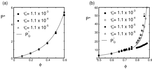
Figure 1: The reduced pressure $P^{*}$ as a function of the area fraction $\phi$ in the monodisperse system with $e=0.999$, for different $\tau_{c}^{*}$, as given in the inset, and for $\phi<0.6$ (a) and $\phi>0.5$ (b).

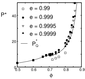
Figure 2: The reduced pressure $P^{*}$ as a function of the area fraction $\phi$ in the monodisperse system with $\tau_{c}^{*}=1.11\times 10^{-5}$ and different $e$, as given in the inset.

In order to check the possibility that the restitution coefficient is the reason for the deviation between the numerical data and $P_{Q}^{*}$ in Fig. 1(b), we plot $P^{*}$ for different $e$, for $\tau_{c}^{*}=1.11\times 10^{-5}$ in Fig. 2. At high densities, for inelastically interacting particles, $e=0.99$, the stress is considerably smaller than predicted by $P^{*}_{Q}$, while for more elastic particles, we observe a higher stress. Only the almost elastic case $e=0.9999$ is close to the prediction.

The low pressure for $e=0.99$ is due to the existence of a shear-band – see below. For all other situations, no shear-band is observed, however, different patterns of defect lines in the crystal are evidenced for $e=0.9990$ and $e=0.9995$, while an almost perfect crystal is observed for $e=0.9999$, where slip-lines appear. It should be noted that the positions of the slip-lines (shear-bands of width $W=d$) don’t move in the steady state of one sample, but vary among different samples.

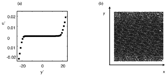
Figure 3: (a) The scaled velocity $u^{\prime}=u/(\sigma_{0}/\sqrt{m/k})$ in $x$ direction as a function of $y^{\prime}=y/\sigma_{0}$, for $\phi=0.84$, $\tau_{c}^{*}=1.11\times 10^{-5}$, and $e=0.99$. (b) Snapshot of the monodisperse system from (a).

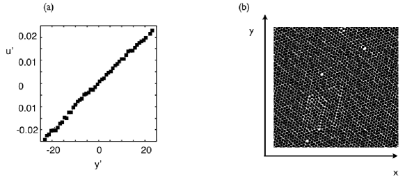
Figure 4: (a) The scaled velocity $u^{\prime}$ (like in Fig. 3) for $\phi=0.84$, $\tau_{c}^{*}=1.11\times 10^{-5}$, and $e=0.999$. (b) Snapshot of the monodisperse system from (a).

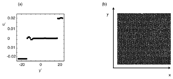
Figure 5: (a) The scaled velocity $u^{\prime}$ (like in Fig. 3) for $\phi=0.84$, $\tau_{c}^{*}=1.11\times 10^{-5}$, and $e=0.9999$. (b) Snapshot of the monodisperse system from (a).

We have confirmed the existence of shear-bands for $\phi>0.7$ with $e=0.99$ in Fig. 3. We plot the velocity $u(y)$ in $x$ direction as a function of $y$ for $\phi=0.76$, $\tau_{c}^{*}=1.11\times 10^{-5}$, and $e=0.99$ in Fig. 3 (a), where the velocity gradient exists only in the regions $y/\sigma_{0}<-20$ or $y/\sigma_{0}>20$. The apparent inhomogeneity is observed in the snapshot of the system, see Fig. 3(b). On the other hand, such a shear-band could not be observed for the case of $e=0.999$. Note that the shear-band formation in our system is different from that for the dilute case [60] in which dense strips align at 45 degrees relative to the streamwise direction. Fig. 4 shows that the system is in an uniformly sheared state with some density fluctuations, see Fig. 4(b). Actually, here deformations take place irregularly and localized – together with defects and slip planes – so that the velocity profile looks smooth and linear only after long-time (or ensemble) averaging. For the case of $e=0.9999$, almost perfect crystallization is observed, but slip-lines exist, see Figs. 5(a) and (b).

This is in conflict with the observations of Ref. Luding09, where shear-bands were observed at densities around $\phi\approx 0.70$, $\phi\approx 0.73$, and $\phi\approx 0.78$, for $e\geq 0.99$, $e=0.95$, and $e=0.90$, respectively. In this paper, for the case of $e=0.999$, no shear band is observed, however, in the simulation of the sheared inelastically interacting rigid-disks with $e=0.998$ in Ref. Luding09, a shear band was reported.

We identify two differences between the systems in this paper and Ref. Luding09. The first difference is the softness of the disks that, however, should not affect the results as long as we are close to the rigid-disk limit. The second difference is the protocol to obtain a sheared steady state with density $\phi$. In this paper, first an equilibrium state with density $\phi$ is prepared and then shear flow and dissipation between the particles is switched on to obtain the sheared steady state. In contrast, in Ref. Luding09, the system of sheared inelastically interacting disks was studied by slowly but continuously increasing the density $\phi$.

The dimensionless viscosity $\eta^{*}$ for monodisperse systems with $e=0.999$, and different $\tau^{*}_{c}$ is shown in Fig. 6. We note that both $P^{*}$ and $\eta^{*}$ converge for more rigid disks $\tau_{c}^{*}\to 0$, but not to the empirical expression $\eta_{L}^{*}$ from Eq. (8). It can be used in a wide range of $\phi$, as one can see in Fig. 6(b), but – even though behaving qualitatively similar – the numerical data clearly deviate from $\eta_{L}^{*}$: For $\phi>0.7$, in the rigid-disk case, $\eta_{L}^{*}$ diverges at $\phi_{\eta}=0.71$, whereas $\eta^{*}$ in the near-rigid case exponentially grows like the Vogel-Fulcher law, which remains finite above $\phi_{\eta}$.

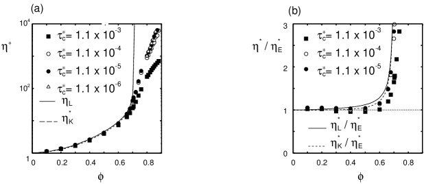
Figure 6: (a) The dimensionless viscosity $\eta^{*}$ as a function of the area fraction $\phi$ in the monodisperse system for $e=0.999$, and different $\tau^{*}_{c}$ as given in the inset. (b) $\eta^{*}/\eta_{E}^{*}$ as a function of the area fraction from the same simulations as in (a).

The difference between the numerical data for $\eta^{*}$ and $\eta^{*}_{L}$ results from both elasticity and dissipation, as shown in Fig. 7, where the dependence of $\eta^{*}$ on $\phi$ for $\tau_{c}^{*}=1.11\times 10^{-5}$ and different coefficients of restitution $e$ are plotted. The viscosity $\eta^{*}$, like the pressure $P^{*}$, approach $\eta^{*}_{L}$ and $P^{*}_{Q}$ in the elastic limit $e\to 1$, i.e., they converge to the results of the elastic rigid-disk system. It should be noted that Figs. 6(a) and 7(a) suggest that the singularity around $\phi=\phi_{\eta}$ is an upper limit, only realized in the rigid disk limit and for $e\rightarrow 1$. As will be discussed below, for given $\tau_{c}^{*}$ and $e$, the simulations deviate more and more from the rigid disk case with increasing density. The smaller $\tau_{c}^{*}$, i.e., the stiffer the disks, the better is the upper limit approached – but for finite dissipation and for near-rigid disks, there is always a finite density where the elasticity (softness) becomes relevant and leads to deviations from the upper limit. Above that density, it seems that the divergence of the viscosity takes place at the same point as the pressure, and another inverse power law can be a fitting function for $\phi<\phi_{\eta}$.

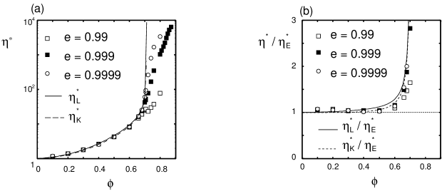
Figure 7: The dimensionless viscosity $\eta^{*}$ as a function of the area fraction $\phi$ in the monodisperse system for $\tau_{c}^{*}=1.11\times 10^{-5}$ and $e=0.99$, $0.999$, $0.9999$. (b) $\eta^{*}/\eta_{E}^{*}$ as a function of the area fraction from (a).

In rigid-disk systems, the coordination number $Z$ should be identical to zero because the contacts between the particles are instantaneous. Hence, in the rigid-disk limit of soft-disks, it is expected that the coordination number $Z$ vanishes, which is confirmed by Fig. 8(a). Here, it should be noted that the coordination number $Z$ is almost identical to the dimensionless number $\tau_{cE}^{*}$ [56]. Indeed the relationship $Z\approx\tau_{cE}^{*}$ can be verified in Fig. 8(b), where we plot the ratio $\tau_{cE}^{*}/Z$ as function of the area fraction $\phi$ for monodisperse systems with $e=0.999$ and several $\tau_{c}^{*}$. Here, we have measured the coordination number as

$$Z=\sum_{i}\sum_{j\neq i}\langle\Theta(\sigma_{ij}-r_{ij})\rangle/N~{}.$$ (33)

If we use the mean-field picture, we can understand the relation $Z\approx\tau_{cE}^{*}$ as shown in Appendix A.

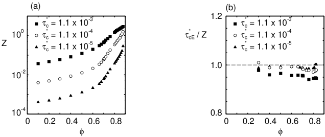
Figure 8: (a) The coordination number $Z$ plotted as function of the area fraction $\phi$ for monodisperse systems with $e=0.999$ for several $\tau_{c}^{*}$ values. (b) $\tau_{cE}^{*}/Z$ plotted as function of the area fraction $\phi$ from the same simulations as in (a).

We also show the scaled temperature $T^{*}$ for the soft-sphere monodisperse system in Fig. 9. As expected, $T^{*}$ approaches the empirical expression $T_{K}^{*}$ in Eq. (11). This result also supports our conjecture that the rigid-disk limit of the soft-disk assemblies coincides with the rigid-disk system when the coefficient of restitution $e$ is sufficiently close to unity.

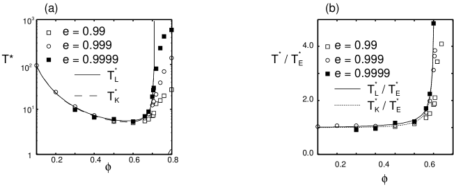
Figure 9: (a) The scaled temperature $T^{*}$ as a function of the area fraction $\phi$ for the monodisperse system at $\tau_{c}^{*}=1.11\times 10^{-5}$ and different $e$. (b) $T^{*}/T^{*}_{E}$ as a function of the area fraction $\phi$ from the same simulations as in (a).

3.3 Poly-disperse systems

In order to understand the polydisperse situation, we also study systems with different $\tau_{c}^{*}$ and different $e$ values – as in the previous subsection. The reduced pressure $P^{*}$ and the dimensionless viscosity $\eta^{*}$ are almost independent of $\tau_{c}^{*}$ and $e$ for moderate densities ($\phi<0.8$), as shown in Fig. 10, where $P^{*}$ and $\eta^{*}$ are plotted as functions of the area fraction $\phi$. For low densities, the simulation results of $P^{*}$ agree with the scaling given by $P_{d}^{*}$, while the asymptotic scaling behavior of $\eta^{*}$ is described by $\eta_{d}^{*}$ only above $\phi\simeq 0.8$. Here, we have used $\phi_{\rm max}=0.841$ for $P^{*}$ and $\eta^{*}$ in Eqs. (13) and (14).

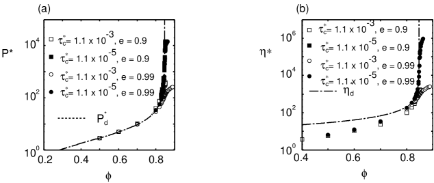
Figure 10: (a) The dimensionless pressure $P^{*}$ as a function of the area fraction $\phi$ for polydisperse systems with several different $\tau^{*}_{c}$ and $e$, where we have used $\phi_{\rm max}=0.841$ for $P_{d}^{*}$ and $\eta^{*}_{d}$. The prefactor for $P_{d}^{*}\propto(\phi_{\rm max}-\phi)^{-1}$ is chosen as $2\phi_{\rm max}$ [46, 48, 24]. (b) The dimensionless viscosity $\eta^{*}$ as a function of the area fraction $\phi$ from the same simulations as in (a). Here, we have used the prefactor 7.0 for $\eta_{d}^{*}\propto(\phi_{\rm max}-\phi)^{-1}$.

However, when looking more closely, there are distinct differences between $P^{*}$ and $P_{d}^{*}$, and between $\eta^{*}$ and $\eta^{*}_{d}$ for $\phi>0.83$. In Fig. 11, $P^{*}$ and $\eta^{*}$ are plotted from polydisperse systems with rather strong dissipation, $e=0.9$, where we have used particular values for $\phi_{\rm max}=0.841$ and $\phi_{J}=0.8525$ in order to visualize their different behavior. Although $P^{*}$ is still finite for $\phi>\phi_{\rm max}$ in the hard disk limit, even for the smallest $\tau^{*}_{c}$ values, both $P_{d}^{*}$ and $\eta_{d}^{*}$ diverge at $\phi_{\rm max}$ as $(\phi_{\rm max}-\phi)^{-1}$. On the other hand, in the same high density range, $P^{*}$ and $\eta^{*}$ are consistent with $P_{J}^{*}$ (21) and $\eta_{J}^{*}$ (22) [39, 40] in the rigid-disk limit ($\tau_{c}^{*}=1.11\times 10^{-6}$), as will be shown below.

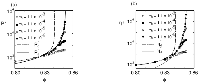
Figure 11: (a) The dimensionless pressure $P^{*}$ as a function of the area fraction $\phi$ for the polydisperse system for $e=0.9$ and several $\tau^{*}_{c}$. (b) The dimensionless viscosity $\eta^{*}$ as a function of the area fraction $\phi$ in the polydisperse system from the same simulations as those in (a). Here, we have used $\phi_{J}=0.8525$ for $P^{*}_{J}$ and $\eta^{*}_{J}$, and $\phi_{\rm max}=0.841$ for $P^{*}_{d}$ and $\eta^{*}_{d}$. The prefactors for $P_{d}^{*}\propto(\phi_{\rm max}-\phi)^{-1}$ and $\eta_{d}^{*}\propto(\phi_{\rm max}-\phi)^{-1}$ are $2\phi_{\rm max}$ and $7.0$, respectively. For $P_{J}^{*}\propto(\phi_{J}-\phi)^{-2}$ and $\eta_{J}^{*}\propto(\phi_{J}-\phi)^{-3}$, the prefactors are chosen as $0.07$ and $0.002$, respectively.

In order to verify whether the critical behavior of $P^{*}$ and $\eta^{*}$ can be described by $P_{J}^{*}$ and $\eta_{J}^{*}$, we plot $P^{*}$ and $\eta^{*}$ as functions of $\phi_{J}-\phi$ in Fig. 12. Here, we plot only the data for $\phi<\phi_{J}$ because we discuss the scaling behavior of $P^{*}$ and $\eta^{*}$ in the unjammed regime in this paper. $P^{*}$ and $\eta^{*}$ in the rigid-disk limit approach $P_{J}^{*}$ and $\eta_{J}^{*}$, which satisfy $(\phi_{J}-\phi)^{-2}$ and $(\phi_{J}-\phi)^{-3}$, respectively.

It should be noted that the plateaus in Fig. 12, close to the jamming transition point, for $\phi\simeq\phi_{J}$, can also be predicted from the scaling theory, by rewriting Eqs. (15)–(19). More specifically, the arguments are taken to the power $-1/\alpha$:

$$T=\dot{\gamma}^{x_{\Phi}/\alpha}{\cal T}^{\prime}_{\pm}\left(\frac{|\Phi|}{\dot{\gamma}^{1/\alpha}}\right),\ S=\dot{\gamma}^{y_{\Phi}/\alpha}{\cal S}^{\prime}_{\pm}\left(\frac{|\Phi|}{\dot{\gamma}^{1/\alpha}}\right),\ P=\dot{\gamma}^{y_{\Phi}^{\prime}/\alpha}{\cal P}^{\prime}_{\pm}\left(\frac{|\Phi|}{\dot{\gamma}^{1/\alpha}}\right),$$ (34)

where we have introduced ${\cal T}^{\prime}_{\pm}(x)=x^{-x_{\Phi}}{\cal T}_{\pm}(x^{-\alpha})$, ${\cal S}^{\prime}_{\pm}(x)=x^{-y_{\Phi}}{\cal S}_{\pm}(x^{-\alpha})$, and ${\cal P}^{\prime}_{\pm}(x)=x^{-y^{\prime}_{\Phi}}{\cal P}_{\pm}(x^{-\alpha})$. The scaling functions satisfy $\lim_{x\to 0}{\cal T}^{\prime}_{\pm}(x)=\lim_{x\to 0}{\cal S}^{\prime}_{\pm}(x)=\lim_{x\to 0}{\cal P}^{\prime}_{\pm}(x)=const.$ Substituting these relations into Eqs. (1) (2), with Eqs. (19), $\eta=S/\dot{\gamma}$, $\Delta=1$, and the definition of $\tau_{c}^{*}$ given by Eq. (26), the scaling relations of $P^{*}$ and $\eta^{*}$ are obtained as

$$P^{*}=\tau_{c}^{*-4/5}{\cal P}^{*}_{\pm}\left(\frac{|\Phi|}{\tau_{c}^{*2/5}}\right),\ \eta^{*}=\tau_{c}^{*-6/5}{\cal H}^{*}_{\pm}\left(\frac{|\Phi|}{\tau_{c}^{*2/5}}\right).$$ (35)

Here, the scaling functions satisfy $\lim_{x\to 0}{\cal P}^{*}_{\pm}(x)=\lim_{x\to 0}{\cal H}^{*}_{\pm}(x)=const.$ Therefore, the plateau for $P^{*}$ and $\eta^{*}$ in Fig. 12 should be proportional to $(1/\tau_{c}^{*})^{4/5}$ and $(1/\tau_{c}^{*})^{6/5}$, respectively, which is confirmed by Fig. 13, where we plot $P^{*}\tau_{c}^{*4/5}$ and $\eta^{*}\tau_{c}^{*6/5}$ as a function of $(\phi_{J}-\phi)/\tau_{c}^{*2/5}$.

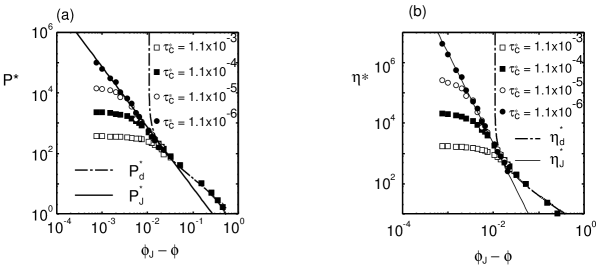
Figure 12: (a) The reduced pressure $P^{*}$ plotted as a function of $\phi_{J}-\phi$ for polydisperse systems with $e=0.9$ and several $\tau^{*}_{c}$ based on the simulations used for Fig. 11. (b) The dimensionless viscosity $\eta^{*}$ from the same simulations as those in (a). Here, we have used $\phi_{J}=0.8525$ for $P^{*}_{J}$ and $\eta^{*}_{J}$, and $\phi_{\rm max}=0.841$ for $P^{*}_{d}$ and $\eta^{*}_{d}$.

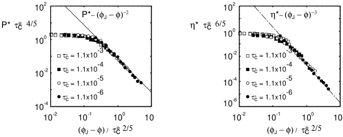
Figure 13: (a) Plots of $P^{*}\tau_{c}^{*4/5}$ versus $(\phi_{J}-\phi)/\tau_{c}^{*2/5}$ for polydisperse systems with $e=0.9$ and several $\tau^{*}_{c}$. (b) Plots of $\eta^{*}\tau_{c}^{*6/5}$ versus $(\phi_{J}-\phi)/\tau_{c}^{*2/5}$ for polydisperse systems with $e=0.9$ and several $\tau^{*}_{c}$.

Whether the simulation pressure is described by $P_{d}^{*}$ or $P_{J}^{*}$, and whether the viscosity is given by $\eta_{d}^{*}$ or $\eta_{J}^{*}$, strongly depends on the coefficient of restitution $e$. In Figs. 14–16, we plot $P^{*}$ and $\eta^{*}$ as functions of $\phi$ for various $e$, involving the very high dissipation case $e=0.1$, an intermediate case $e=0.99$, and a low dissipation case $e=0.998$. Using fitting values $\phi_{\rm max}=0.841$, $0.848$, and $0.851$, based on a fit starting from very low densities, corresponding to various $e=0.1$, $0.99$ and $0.998$, respectively, we can approximate the data of $P^{*}$ best by $P_{d}^{*}=2\phi_{\rm max}/(\phi_{\rm max}-\phi)$. On the other hand, we assume that $\phi_{J}$ is independent of $e$, and fix $\phi_{J}=0.8525$ for all $e$, as confirmed this by our numerical simulations.

Even in the case of strong inelasticity ($e=0.1$), as shown in Fig. 14, $P_{J}^{*}$ and $\eta_{J}^{*}$ characterize the behavior of $P^{*}$ and $\eta^{*}$ near the jamming transition point, while $P_{d}^{*}$ and $\eta_{d}^{*}$ deviate for $\phi>0.83$. The range where $P_{J}^{*}$ and $\eta_{J}^{*}$ characterize the pressure and the viscosity becomes narrower as $e\to 1$, while the range of validity of $P_{d}^{*}$ becomes wider, as shown in Figs. 15 and 16. For $e=0.998$ (Fig. 16), the difference between $P_{d}^{*}$ and $P_{J}^{*}$ appears only in a small region of $\phi$ which is shown in Fig. 17.

Since the scaling behaviors of $P^{*}$ and $\eta^{*}$ agree with $P_{J}^{*}$ and $\eta_{J}^{*}$ near $\phi_{J}$, we conclude that the critical behavior for inelastic near-rigid systems is well described by $P_{J}^{*}$ and $\eta_{J}^{*}$, as proposed in Refs. Otsuki:PTP,Otsuki:PRE. The scaling plot in Fig. 13 supports the validity of the critical behaviors concerning both the plateaus and the lower densities. However, such predictions cannot be used for almost elastic and perfectly elastic systems, neither mono- or polydisperse, whose critical behavior is described by $P_{d}^{*}$ and $\eta_{d}^{*}$ instead.

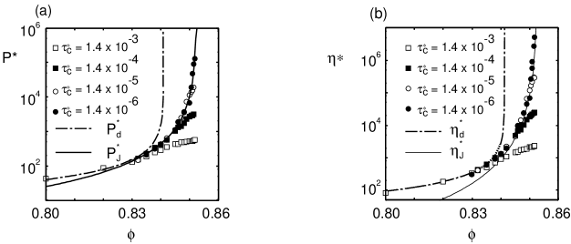
Figure 14: (a) The reduced pressure $P^{*}$ as a function of the area fraction $\phi$ for the polydisperse system with $e=0.1$ and several $\tau^{*}_{c}$. (b) The dimensionless viscosity $\eta^{*}$ from the same data as those in (a). We have used $b=0.07$ and $\phi_{J}=0.8525$ for $P_{J}$ and $\eta_{J}$, and $\phi_{\rm max}=0.841$ for $P_{d}$ and $\eta_{d}$. We used $\phi_{J}=0.8525$ for $P^{*}_{J}$ and $\eta^{*}_{J}$, and $\phi_{\rm max}=0.841$ for $P^{*}_{d}$ and $\eta^{*}_{d}$ The prefactors for $P_{d}^{*}\propto(\phi_{\rm max}-\phi)^{-1}$ and $\eta_{d}^{*}\propto(\phi_{\rm max}-\phi)^{-1}$ are $2\phi_{\rm max}$ and $7.0$, respectively. The prefactors for $P_{J}^{*}\propto(\phi_{J}-\phi)^{-2}$ and $\eta_{J}^{*}\propto(\phi_{J}-\phi)^{-3}$ are given by $0.07$ and $0.002$, respectively.

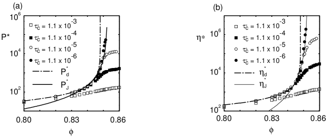
Figure 15: (a) The reduced pressure $P^{*}$ as a function of the area fraction $\phi$ for the polydisperse system with $e=0.99$ and several $\tau^{*}_{c}$. (b) The dimensionless viscosity $\eta^{*}$ obtained from the same data as those in (a). We have used $\phi_{J}=0.8525$ for $P_{J}$ and $\eta_{J}$, and $\phi_{\rm max}=0.848$ for $P_{d}$ and $\eta_{d}$. The prefactors for $P_{d}^{*}\propto(\phi_{\rm max}-\phi)^{-1}$ and $\eta_{d}^{*}\propto(\phi_{\rm max}-\phi)^{-1}$ are $2\phi_{\rm max}$ and $10.0$, respectively. The prefactors for $P_{J}^{*}\propto(\phi_{J}-\phi)^{-2}$ and $\eta_{J}^{*}\propto(\phi_{J}-\phi)^{-3}$, are $0.035$ and $0.0015$, respectively.

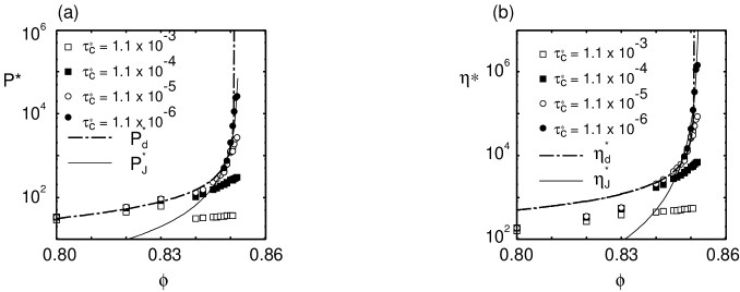
Figure 16: (a) The reduced pressure $P^{*}$ as a function of the area fraction $\phi$ for the polydisperse system for $e=0.998$ and several $\tau^{*}_{c}$. (b) The dimensionless viscosity $\eta^{*}$ obtained from the same data as those in (a). We have used $\phi_{J}=0.8525$ for $P^{*}_{J}$ and $\eta_{J}$, and $\phi_{\rm max}=0.851$ for $P^{*}_{d}$ and $\eta_{d}$. The prefactors for $P_{d}^{*}\propto(\phi_{\rm max}-\phi)^{-1}$ and $\eta_{d}^{*}\propto(\phi_{\rm max}-\phi)^{-1}$ are $2\phi_{\rm max}$ and $25.0$, respectively. The prefactors for $P_{J}^{*}\propto(\phi_{J}-\phi)^{-2}$ and $\eta_{J}^{*}\propto(\phi_{J}-\phi)^{-3}$, are $0.01$ and $0.001$, respectively.

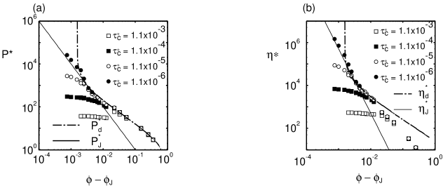
Figure 17: (a) The reduced pressure $P^{*}$ plotted as a function of $\phi_{J}-\phi$ for polydisperse systems with $e=0.998$ and several $\tau^{*}_{c}$ based on the simulations used for Fig. 16. (b) The dimensionless viscosity $\eta^{*}$ obtained from the same simulations as those in (a). We have used $\phi_{J}=0.8525$ for $P^{*}_{J}$ and $\eta_{J}$, and $\phi_{\rm max}=0.851$ for $P^{*}_{d}$ and $\eta_{d}$. The prefactors for $P_{d}^{*}\propto(\phi_{\rm max}-\phi)^{-1}$ and $\eta_{d}^{*}\propto(\phi_{\rm max}-\phi)^{-1}$ are $2\phi_{\rm max}$ and $25.0$, respectively. The prefactors for $P_{J}^{*}\propto(\phi_{J}-\phi)^{-2}$ and $\eta_{J}^{*}\propto(\phi_{J}-\phi)^{-3}$, are $0.01$ and $0.001$, respectively.

3.4 Dimensionless numbers and a criterion for the two scaling regimes

In Sec. 3.3, we reported a crossover from the region satisfying Eqs. (13) and (14) to the region satisfying Eqs. (21) and (22). Figure 18 presents a schematic phase diagram in the plane of the restitution coefficient $e$ and the area fraction $\phi$, where -1 denotes the region satisfying the scaling relations given by Eqs. (13) and (14), and OH denotes the region satisfying the scalings given by Eqs. (21) and (22). For each $e$, the high density region satisfies Eqs. (21) and (22), while the low density region satisfies the scalings given by Eqs. (13) and (14). As the restitution coefficient approaches unity, the region of OH becomes “narrower”, and disappears in the elastic limit.

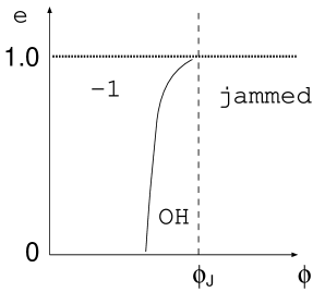
Figure 18: A schematic phase diagram of the region (-1) satisfying Eqs. (13), (14) and the region (OH) satisfying Eqs. (21), (22).

Now, let us discuss which of the dimensionless numbers $\tau_{E}^{*}$, $\tau_{cE}^{*}$, $\tau_{\omega}^{*}$ or $\tau_{c\omega}^{*}$ can be used as the criterion to distinguish between the two scaling regimes. It should be noted that the dimensionless number for the criterion must be a monotonic function of $\phi$, because the scaling relations Eqs. (13) and (14) appear in the higher density region and the scaling relations Eqs. (21) and (22) appear in the lower density region regardless to other parameters.

First, let us consider $\tau_{E}^{*}$. We expect that $\tau_{E}^{*}<A$ or $\tau_{E}^{*}>A$ is the criterion for the scaling regime given by (21) and (22), where $A$ is a constant. However, since $\tau_{E}^{*}$ is not a monotonic function of the area fraction $\phi$ and the restitution coefficient $e$, as shown in Fig. 19(a), we conclude that neither $\tau_{E}^{*}<A$ or $\tau_{E}^{*}>A$ is appropriate for the criterion.

Similar to the case of $\tau_{E}^{*}$, $\tau_{cE}^{*}$ in not a monotonic function of $\phi$ and $e$, as shown in Fig. 19(b). Therefore, we conclude that $\tau_{cE}^{*}$ is not an appropriate dimensionless time for the criterion.

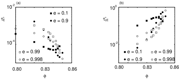
Figure 19: (a) $\phi$ dependence on $\tau_{E}^{*}$ and (b) $\phi$ dependence on $\tau_{cE}^{*}$, for various $e$, from simulations with $\tau_{c}^{*}=1.1\times 10^{-5}$.

Finally, let us consider $\tau_{\omega}^{*}$ and $\tau_{c\omega}^{*}$, which are respectively related with $\tau_{E}^{*}$ and $\tau_{cE}^{*}$ as $\tau_{\omega}^{*}\approx 2\tau_{E}^{*}/(1-e^{2})$ and $\tau_{c\omega}^{*}\approx(1-e^{2})\tau_{cE}^{*}/2$ in the collisional regime, but their dependency on $\phi$ and $e$ differs from those of $\tau_{E}^{*}$ and $\tau_{cE}^{*}$, as shown in Figs. 20(a) and 20(b). Both $\tau_{\omega}^{*}$ and $\tau_{c\omega}^{*}$ are monotonic functions of $\phi$ and $e$. Since Eqs. (21) and (22) are satisfied in the high density region and $\tau_{\omega}^{*}$ and $\tau_{c\omega}^{*}$ are respectively decreasing and increasing functions of the density $\phi$, $\tau_{\omega}^{*}<A$ and $\tau_{c\omega}^{*}>A$ are the possible conditions for the scaling given by Eqs. (21) and (22). These conditions are also consistent with the dependencies of $\tau_{\omega}^{*}$ and $\tau_{c\omega}^{*}$ on $e$. Indeed, $\tau_{\omega}^{*}$ increases as the restitution constant increases, and $\tau_{c\omega}^{*}$ is a decreasing function of $e$. This means that the regions satisfying $\tau_{\omega}^{*}<A$ and $\tau_{c\omega}^{*}>A$ are narrower as the restitution constant increases, which is consistent with the numerical observation. Therefore, $\tau_{\omega}^{*}<A$ and $\tau_{c\omega}^{*}>A$ are the only two possible candidates to characterize the system with respect to their scaling behavior. It should be noted that $\tau_{c\omega}^{*}$ tends to zero in the hard disk limit $\tau_{c}^{*}\to 0$. In this sense, to use $\tau_{c\omega}^{*}$ might involve a conceptual difficulty, even though $\tau_{c\omega}^{*}$ is finite in the jamming region.

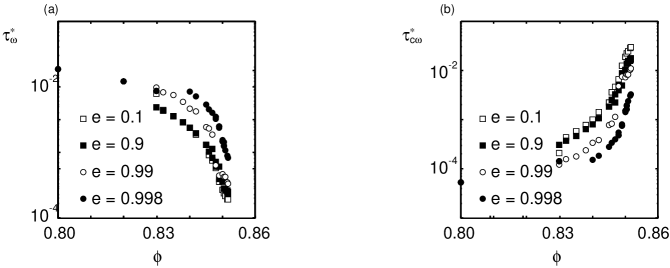
Figure 20: (a) $\phi$ dependence on $\tau_{\omega}^{*}$ and (b) $\phi$ dependence on $\tau_{c\omega}^{*}$ for various $e$, from simulations with $\tau_{c}^{*}=1.1\times 10^{-5}$.

4 Conclusion and Discussion

In conclusion, we have investigated the dimensionless pressure $P^{*}$ and the dimensionless viscosity $\eta^{*}$ of two-dimensional soft disk systems and have payed special attention to the rigid-disk limit of inelastically interacting systems, while near-rigid disks still have some elasticity (“softness”).

For monodisperse systems, as the system approaches the elastic limit, $e\to 1$, both $P^{*}$ and $\eta^{*}$ for $\phi<\phi_{\eta}=0.71$ approach the results of elastic rigid-disk systems, where the viscosity increases rapidly around $\phi=\phi_{\eta}$ due to ordering (crystallization) effects, while the pressure for $\phi>\phi_{\eta}$ is still finite [36]. This result is consistent with Ref. Mitarai, where Mitarai and Nakanishi suggested that the behavior of soft-disks in dilute collisional flow converges to that of rigid-disks in the rigid-disk limit.

For polydisperse systems, both $P^{*}$ and $\eta^{*}$ behave as $(\phi_{J}-\phi)^{-2}$ and $(\phi_{J}-\phi)^{-3}$ near the jamming transition point, $\phi_{J}>\phi_{\eta}$, as predicted in Refs. Otsuki:PTP,Otsuki:PRE. However, as the restitution coefficient $e$ approaches unity, the scaling regime becomes narrower, and the exponents for the divergence of $P^{*}$ and $\eta^{*}$ approach values close to $-1$ in the almost elastic case.

From these results, we conclude that the predictions for the inelastic soft-disk systems in Refs. Otsuki:PTP,Otsuki:PRE are applicable to the inelastic near-rigid disk systems below the jamming transition point, but the prediction cannot be used for almost elastic rigid-disk systems. It seems that $\tau_{c\omega}^{*}$ and $\tau_{\omega}^{*}$ are the only two possible candidates to characterize the criterion of this crossover. In other words, the energy dissipation rate and the shear rate set the two competing time-scales that define the dimensionless number $\tau_{\omega}^{*}$. For $\tau_{\omega}^{*}\ll 0.01$ the near-rigid, dissipative scaling regime occurs, while for $\tau_{\omega}^{*}\gg 0.01$ the rigid, elastic scaling regime is realized.

In three-dimensional sheared inelastic soft-sphere systems [39, 40], even in monodisperse cases, there is no indication of the strong ordering transition, and the scaling given in Eqs. (21) and (22) seems to be valid. However, a direct comparison of near-rigid sphere with rigid sphere simulations in the spirit of the present study is unavailable to our knowledge.

We restricted our interest to frictionless particles. When the particles have friction, the scaling relations for the divergence of the viscosity and the pressure may be different, as will be discussed elsewhere. Furthermore, the very soft or high shear rate regime also needs further attention in both 2D and 3D.

Appendix A The relation between $Z$ and $\tau_{cE}^{*}$

In this appendix, we derive the relation between $Z$ and $\tau_{cE}^{*}$ as

$$Z\simeq t_{c}t_{E}^{-1}=\tau_{cE}^{*},$$ (36)

which corresponds to the difference between counting contacts vs. counting of collisions in the simulations. (Note that counting contacts is not possible for rigid disks, since the probability to observe a $t_{c}=0$ contact at any given snapshot in time is zero.)

Since the ensemble average in Eq. (33) is independent of $i$ and $j$, without loss of generality, one can set $i=1$ and $j=2$, and obtains

$$\sum_{i}\sum_{j\neq i}\langle\Theta(\sigma_{ij}-r_{ij})\rangle=N(N-1)\langle\Theta(\sigma_{12}-r_{12})\rangle.$$ (37)

Substituting this equation into Eq. (33), we obtain

$$Z=(N-1)\langle\Theta(\sigma_{12}-r_{12})\rangle.$$ (38)

On the other hand, $t_{E}^{-1}$ is defined as the frequency of collisions per particle:

$$t_{E}^{-1}=\sum_{j\neq i}\left\{\lim_{T\to\infty}\frac{1}{T}n_{c,ij}(T)\right\},$$ (39)

where $n_{c,ij}(t)$ is the number of the collisions between grains $i$ and $j$ until time $T$. Since $\lim_{T\to\infty}n_{c,ij}(T)/T$ is independent of $j$, like above, we obtain

$$t_{E}^{-1}=(N-1)\left\{\lim_{T\to\infty}\frac{1}{T}n_{c,12}(T)\right\}$$ (40)

In order to derive Eq. (36), the ensemble average in Eq. (38) is replaced by the time average as

$$Z=(N-1)\lim_{T\to\infty}\frac{1}{T}\int_{0}^{T}dt\ \Theta(\sigma_{12}-r_{12}(t)),$$ (41)

where $r_{ij}(t)$ is the distance between grains $i$ and $j$ at time $t$. Since $\Theta(\sigma_{12}-r_{12}(t))=1$ for the duration $t_{c}$ after a collision begins, the integral in Eq. (41) is estimated as $n_{c,12}(T)\ t_{c}$, which yields

$$Z = (N-1)\lim_{T\to\infty}\frac{1}{T}\{n_{c,12}(T)t_{c}\}$$ (42)

$$= \left[(N-1)\left\{\lim_{T\to\infty}\frac{1}{T}n_{c,12}(T)\right\}\right]t_{c}.$$

Finally, substituting Eq. (40) into this equation, gives Eq. (36) so that we can apply Eq. (33).

References

• [1] I. S. Aronson and Lev S. Tsimring, Rev. Mod. Phys. 78 (2006), 641.
• [2] O. Pouliquen, Phys. Fluids 11 (1999), 542.
• [3] L.E. Silbert, D. Ertaş, G. S. Grest, T. C. Halsey, D. Levine and S. J. Plimpton, Phys. Rev. E 64 (2001), 051302.
• [4] J. F. Lutsko, Phys. Rev. E 63 (2001), 061211.
• [5] M. Alam and S. Luding, Phys. Fluids 15 (2003), 2298.
• [6] GDRMiDi, Eur. Phys. J. E 14 (2004), 341.
• [7] J. F. Lutsko, Phys. Rev. E 70 (2004), 061101.
• [8] N. Mitarai and H. Nakanishi, Phys. Rev. Lett. 94 (2005), 128001.
• [9] V. Kumaran, Phys. Rev. Lett. 96 (2006), 258002.
• [10] A. V. Orpe and A. Kudrolli, Phys. Rev. Lett. 98 (2007), 238001.
• [11] K. Saitoh and H. Hayakawa, Phys. Rev. E 75 (2007), 021302.
• [12] N. Mitarai and H. Nakanishi, Phys. Rev. E 75 (2007), 031305.
• [13] H. Hayakawa and M. Otsuki, Phys. Rev. E 76 (2007), 051304 .
• [14] H. Hayakawa and M. Otsuki, Prog. Theor. Phys. 119 (2008), 381.
• [15] A. V. Orpe, V. Kumaran, K. A. Reddy and A. Kudrolli, Europhys. Lett. 84 (2008), 64003.
• [16] T. Hatano, J. Phys. Soc. Jpn. 77 (2008), 123002.
• [17] V. Kumaran, Phys. Rev. E 79 (2009), 011301, ibid 011302.
• [18] H. Hayakawa and M. Otsuki, Prog. Theor. Phys. Suppl. 178 (2009), 49.
• [19] M. Otsuki and H. Hayakawa, Prog. Theor. Phys. Suppl. 178 (2009), 56.
• [20] M. Otsuki and H. Hayakawa, Rarefied Gas Dynamics: Proceedings of 26th international symposium on rarefied gas dynamics, edited by T. Abe et al. (AIP Conf. Proc. 1084) (2009), 57.
• [21] M. Otsuki and H. Hayakawa, Phys. Rev. E 79 (2009), 021502.
• [22] M. Otsuki and H. Hayakawa, J. Stat. Mech. (2009), L08003,.
• [23] M. Otsuki and H. Hayakawa, to be published in Euro. Phys. J. E (arXiv:0907:4462v2).
• [24] S. Luding (2009), Nonlinearity 22, R101-R146.
• [25] H. Jaeger, S. R. Nagel, and R. P. Behringer, Rev. Mod. Phys. 68 (1996), 1296.
• [26] N. Brilliantov and T. Pöschel, Kinetic Theory of Granular Gases (Oxford University Press, Oxford, 2004).
• [27] J. T. Jenkins and M. W. Richman, Phys. Fluids 28 (1985), 3485.
• [28] J. W. Dufty, A. Santos, and J. J. Brey, Phys. Rev. Lett 77 (1996), 1270.
• [29] A. Santos, J. M. Montanero, J. Dufty, and J. J. Brey, Phys. Rev. E 57 (1998), 1644.
• [30] V. Gárzo and J. W. Dufty, Phys. Rev. E 59 (1999), 5895.
• [31] R. Ramirez, D. Risso, R. Soto, and P. Cordero, Phys. Rev. E 62 (2000), 2521.
• [32] J. J. Brey and D. Cubero, in Granular Gases, edited by T. Pöschel and S. Luding (Springer, New York) (2001), 59.
• [33] I. Goldhirsch, Annu. Rev. Fluid Mech. 35 (2003), 267.
• [34] J. F. Lutsko, Phys. Rev. E 72 (2005), 021306.
• [35] T. Ishiwata, T. Murakami, S. Yukawa, and N. Ito, Int. J. Mod. Phys. C, 15 (2004), 1413.
• [36] R. Garcia-Rojo, S. Luding and J. J. Brey, Phys. Rev. E 74 (2006), 061305.
• [37] E. Khain, Phys. Rev. E 75 (2007), 051310.
• [38] E. Khain, Europhys. Lett. 87 (2009), 14001.
• [39] M. Otsuki and H. Hayakawa Prog. Theor. Phys. 121 (2009), 647.
• [40] M. Otsuki and H. Hayakawa Phys. Rev. E 80 (2009), 011308.
• [41] A. J. Liu and S. R. Nagel, Nature 396 (1998), 21.
• [42] W. Losert, L. Bocquet, T. C. Lubensky, and J. P. Gollub, Phys. Rev. Lett. 85 (2000), 1428.
• [43] P. Olsson and S. Teitel, Phys. Rev. Lett. 99 (2007), 178001.
• [44] W. B. Russel, D. A. Saville, and W. R. Schowalter, Colloidal Dispersions (Cambridge University Press, New York, 1989).
• [45] A. Fingerle and S. Herminghaus, Phys. Rev. E, 77 (2008), 011306.
• [46] S. Luding and O. Strauß, in Granular Gases (Springer, Berlin, 2001) edited by T. Pöschel and S. Luding.
• [47] S. Luding, Phys. Rev. E, 63 (2001), 042201.
• [48] S. Luding, Advances in Complex Systems 4 (2002), 379.
• [49] S. Luding and A. Santos, J. Chem. Phys, 121 (2004), 8458.
• [50] O. Herbst, P. Müller, M. Otto, and A. Zippelius, Phys. Rev. E, 70 (2004), 051313.
• [51] S. Luding and A. Goldshtein, Granular Matter 5 (2003), 159.
• [52] N. Mitarai and H. Nakanishi, Phys. Rev. E 67 (2003), 021301.
• [53] D. Henderson, Molec. Phys., 30 (1975), 971.
• [54] E. Helfand, Phys. Rev. 119 (1960), 1.
• [55] S. Torquato, Phys. Rev. E, 51 (1995), 3170.
• [56] S. Luding and S. McNamara, Granular Matter 1 (1998), 113.
• [57] M. Wyart, L. E. Silbert, S. R. Nagel, and T. A. Witten, Phys. Rev. E 72 (2005), 051306.
• [58] C. S. O’Hern, S. A. Langer, A. J. Liu, and S. R. Nagel, Phys. Rev. Lett. 88 (2002), 075507.
• [59] C. S. O’Hern, L. E. Silbert, A. J. Liu, and S. R. Nagel, Phys. Rev. E 68 (2003), 011306.
• [60] M-L. Tan and I. Goldhirsch, Phys. Fluids 9 (1997), 856.