CAN MULTIBAND OBSERVATIONS CONSTRAIN EXPLANATIONS FOR KNOTTY JETS?

Abstract

One can imagine a number of mechanisms that could be the cause of brighter/fainter segments of jets. In a sense, jets might be easier to understand if they were featureless. However we observe a wide variety of structures which we call “knots”. By considering the ramifications of the various scenarios for the creation of knots, we determine which ones or which classes are favored by the currently available multiwavelength data.

1 Introduction

With the advent of the Chandra X-ray Observatory, sub arcsec resolution became available in the 0.5 to 10 keV band. This technological advance resulted in an increase in the number of sources with detections of X-ray jets and hotspots from a few to close to one hundred. During the last ten years, it became apparent that the conventional wisdom (that knots in jets were the results of internal shocks) was only part of the story. We now realize that for X-ray synchrotron features, any emission region must also be an acceleration region since the timescales for radiative losses of the emitting electrons is much shorter than travel times from one part of the jet to downstream regions. Characteristic loss times for X-ray synchrotron-emitting electrons is ten times shorter than for those responsible for the optical emission.

1.1 Angular resolution vs. physical resolution

One of the main obstacles in comparing features in FRI jets with those in quasar and FRII jets is the large change in physical resolution for a fixed angular resolution. In Table 1 we give the physical resolution corresponding to one arcsec for a sample of sources. Typical angular resolutions for adaptive optics, the VLA, MERLIN, and HST will be 0.1 arcsec and VLBA can provide resolutions of 1 to 10 milli arcsec.

Table 1: Physical size corresponding to one arcsec

Source	redshift	Distance	size	Description
		(Mpc)	(pc)
Cen A		3.5	17	FRI jet
M87	0.00427	16	77	FRI jet
PicA	0.035	152	700	FRII jet and hotspot
CygA	0.056	247	1070	FRII hotspots
3C273	0.158	749	2700	CDQ jet
3C109	0.3056	3338	4500	FRII hotspot
3C263	0.656	3934	7000	LDQ hotspot
3C280	1	6600	8000	FRII hotspots
3C9	2	15850	8500	LDQ jet
1508	4.3	39809	6900	CDQ knot

When we make our calculations for physical parameters of jet knots, we are most likely making gross errors because of this limitation. In fig. 1 we can understand that measuring the size, brightness, intensity, and spectrum of a knot in the M87 jet, or in the jet of Cen A (if it were at the distance of M87), will not provide the data necessary to derive the correct physical parameters for the features we can actually discern in the full resolution X-ray map (bottom panel).

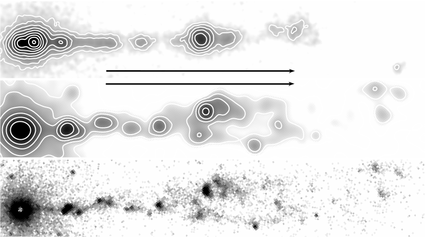
Figure 1: Chandra images of the M87 jet (top) and the Cen A jet (middle and bottom). All images have been rotated and contours increase by factors of two. The scale bars are 1 kpc long. The M87 image has been regridded to one tenth of a native ACIS pixel and smoothed with a Gaussian of FWHM=0.25^′′. The center image is how the Cen A jet would appear if it were at the distance of M87. The bottom image shows the event file which demonstrates that the lower resolution image misses the fine scale structures.

1.2 Is the X-ray emission from quasar jets synchrotron or inverse Compton emission ?

While no definitive answer to this question has been demonstrated, we are reasonably confident that X-ray emission from FRI jets is dominated by synchrotron emission. The remaining contentious issue is the nature of the X-ray emission from quasar jets. If it is synchrotron, then the electrons responsible for the radiation will have energies of $\gamma\geq~{}10^{7}$ ($\gamma$ is the Lorentz factor of the electrons). However, since the energy density of the cosmic microwave background (CMB) in the jet frame will be augmented by $\Gamma^{2}$ ($\Gamma$ is the bulk Lorentz factor of the jet) if $\Gamma\geq$5, the resulting inverse Compton (IC) emission comes from electrons with $\gamma\approx$100. In the former case $E^{2}$ losses (i.e. synchrotron and IC) result in halflives of order a year, whereas in the latter case, it would be $\geq~{}10^{5}$ years, and even longer for regions with magnetic field strengths significantly less than 1 mG (Harris & Krawczynski, 2002). Knot morphology and intensity ratios between radio and X-ray might be quite different depending on which process dominates the X-ray emission.

Synchrotron self-Compton (SSC) emission (for which the target photons are the synchrotron photons) has been found to provide reasonable fits to the spectra of some FRII hotspots, but has generally not been able to explain knot emission (Hardcastle et al., 2004).

2 Multiband Aspects of Knots

For almost all X-ray detections of knots and hotspots, there is a very good correspondence between the X-ray and radio morphologies, but the intensity ratio (X-ray flux divided by the radio flux) varies considerably.

2.1 The X-ray to radio intensity ratio, $R_{\rm{xr}}$

From a study of over a hundred knots and hotspots with both radio and X-ray detections, it has been found that $R_{\rm{xr}}$ lies in the range 1 to 100 for knots of both FRI radio galaxies and quasars whereas most hotspots (both FRII and quasar) have ratios in the range 0.03 to 3 (Harris, Massaro, & Cheung, 2010). In that work we did not sample the much larger number of radio knots with only upper limits of X-ray intensity, so it is quite likely that there are many knots and hotspots with smaller $R_{\rm{xr}}$ values. A priori, if quasar knots were all dominated by IC/CMB X-ray emission, we might have expected to see a clear difference in $R_{\rm{xr}}$ between quasars and FRI knots; instead we find essentially the same range for both classes of sources.

2.2 Offsets and progressions

“Offsets” is a term we use to describe a common (but not universal) property of individual X-ray knots. In many cases, when observed with similar angular resolutions, the brightness of the X-ray image peaks upstream of the lower frequency emissions. This behavior is seen also when comparing optical and radio morphologies, and to the best of our knowledge, always occurs in the sense that the higher frequency peaks upstream of lower frequencies. This subject is discussed in section 3.2.1.1 of Harris & Krawczynski (2006), and several examples are shown.

The term “progressions” is used to describe a systematic change in the overall spectral properties of knots as a function of distance from the nucleus. This has also been covered in Harris & Krawczynski (2006) (section 3.2.1.2). The systematic change is best seen in the ratio of X-ray flux to radio flux and occurs in the sense that the ratio is larger closer to the nucleus. In the case of 3C 273, the ratio changes by two orders of magnitude, whereas for 4C 19.44, the effect is essentially absent.

It is not difficult to see that if a jet segment that behaved like 3C 273 were observed with a single resolution element, it would show a marked offset between the peak of the X-ray compared to the peak of the radio distribution.

Since this sort of effect has been observed over many physical scales, it is likely that synchrotron loss time compared to travel time down the jet is not the only cause of offsets. Rather some other mechanism is at work such as a progressively larger field strength moving down stream. That would produce higher radio intensities as well as perhaps curtailing the production of the very high energy electrons required to produce X-ray synchrotron emission.

3 Mechanisms for Knot Production

Our basic assumption is that a knot is a region of enhanced emissivity which is produced by the jet. It is moving relativistically, but not necessarily at the same velocity as “the jet” (i.e. the velocity of the power flow) (Harris & Krawczynski, 2007). One can imagine several mechanisms for modulating the emissivity along a jet. We consider several possibilities, and suggest a few diagnostics. We do not consider the underlying reasons for the existence of any particular knot at any particular location (i.e. instabilities, interactions with stars, molecular clouds, etc).

3.1 The classical shock scenario

Perhaps the most intuitive explanation for knotty jets is the common notion of a series of shocks. Each would create a new supply of relativistic electrons with a power law distribution determined by the local conditions. The eventual dimming as the shocked plasma is advected down stream can be caused by $E^{2}$ losses or expansion (first power of energy). For $E^{2}$ losses, we expect the lower frequency emissions to last longer, leading to offsets in peak brightness as we move downstream. This is often seen in synchrotron jets; for IC/CMB models, the X-rays come from low energy electrons and should last longer. This behavior is almost never seen, although the end of the jet in 4C19.44 could be an example.

3.2 Adiabatic expansion/contraction

Although quite similar to the shock scenario, there is no shock acceleration as such. The only changes to the electron energy distribution comes from the change in volume of the emitting region. In both the shock case and the change in volume, compression augments the magnetic field and boosts the energy of electrons; expansion reduces synchrotron emission both from the lowering of electron energies, but also by the drop in field strength and moreover, for a fixed observing band, a lower field means you are observing higher energy electrons than previously so you are sampling a segment of the electron spectrum that has many fewer electrons. In the case of IC/CMB X-rays, the emissivity drops only because the normalization factor of the power law distribution of electron energy drops; the change in magnetic field has no effect. Therefore, if expansion were to be the dominent operator for separating adjacent knots, it would mean that the contrast from knot to inter-knot should be greater in the radio/optical than in the X-rays for the IC/CMB model whereas if synchrotron emission dominates the X-ray emissivity, the contrast should be sensibly the same at all frequencies.

3.3 Episodic activity/ejection - power flow is not constant

If kpc jets are similar to pc scale jets, an episodic supply of power to the jet by the SMBH could produce a series of moving knots: knots represent high power intervals of activity, gaps are when the power is low or absent (c.f. the “flip-flop” model of jet formation). If such a mechanism were to be the only formative one, there would have to be two timescales: one for pc scale jets and the other for kpc scale jet knots. Current evidence does not favor this scenario, e.g. the upstream edge of HST-1 (a jet knot close to the nucleus of M87) was thought to have an apparent velocity close to c (downstream blobs were estimated at 6c (Biretta, Sparks, & Macchetto, 1999)) from HST data in the 1990’s. More recently, we measured comparable values at 1.7 GHz (Cheung, Harris, & Stawarz, 2007). However, the upstream edge of HST-1 has not moved during the intervening 10 years, consistent with an interpretation in terms of a stationery shock. We suspect that both estimates for the motion of the upstream edge were centroid shifts caused by the ejection of new components.

3.4 Doppler boosting along a curved trajectory

If the path of a jet changes direction compared to the line of sight, either by thrashing or by a regular (e.g. helical) path, apparent knots can be produced even though the jet itself has a steady power flow. Once the jet has $\Gamma~{}\geq$ a few, moving in and out of the beaming cone can produce the required brightness fluctuations.

The simple expectation is that the radio and X-ray emissions will be coincident: each knot will have the same location and morphology for all wavelengths, i.e. no offsets are expected in the brightness distributions. If the X-rays come from IC/CMB, for most jets the contrast should be higher for the X-rays because of the extra beaming factor of IC/CMB  (Harris & Krawczynski, 2002; Massaro et al., 2009).

3.5 Variable Beaming Factor

If it were possible to “store” jet energy in some other form than in the bulk Lorentz factor, it might be conceivable to envisage a jet with an oscillating value of $\Gamma$. However, if the total energy flow is proportional to $\Gamma$, it would seem difficult to allow $\Gamma$ to drop substantially and then to increase again. If we separate the emitting region from the underlying jet, then the knot’s emission might well decay from a drop in $\Gamma$, and the subsequent knot would have to rely on one of the other possible explanations to generate a new emitting volume.

4 Summary

What we observe is not necessarily “the jet”. “The jet” is whatever it is that carries the energy from the environs of the SMBH to distances of hundreds of kpc. There are a number of possibilities: magnetic field/ Poynting flux, hot or cold protons, or cold pairs. What we see are hot electrons/positrons, but these cannot be the agent that transports the energy since there are inescapable IC losses for electrons with $\gamma\geq$2000 (Harris & Krawczynski, 2007). The larger the $\Gamma$ of the jet (to minimize the local flow of time for $E^{2}$ losses), the larger the IC losses since the effective energy density of the CMB increases as $\Gamma^{2}$. Thus we have the river analogy: “the jet” is a river with smoothly flowing water; the emission we see is like white water produced by turbulence around rocks in the river or waterfalls. The white water is a product of the river and may well be carried along by the river’s flow, but not necessarily with the underlying velocity of the water. All our observations describe the product, not the jet itself. When we see a knot, we see a location where energy is transferred from the jet to produce hot (radiating) electrons. For many knots, the energy transferred is a small fraction of the total power of the jet, whereas for terminal hotspots in FRII radio galaxies, the transfer is complete.

If IC/CMB dominates the X-ray emission, it seems that creating knot structure is a non-trivial problem. Curved trajectories and episodic ejection from the SMBH may be amongst the few viable options, since once a substantial population of low energy electrons is generated, it is difficult to reduce the emissivity and then increase it again.

We suggest a diagnostic of comparing the brightness contrast between the peak intensity of a knot and the preceding and following minimum brightness (the gap between knots). If expansion and contraction is the dominant mechanism for knot production, the synchrotron emission should have a much larger contrast than IC/CMB emission. If however a change in direction of the beaming cone is the principal operative, then the IC/CMB emission should (statistically) display the higher contrast.

References

- Biretta, Sparks, & Macchetto (1999) Biretta, J. A., Sparks, W. B. & Macchetto, F. D. 1999 ApJ 520, 621
- Cheung, Harris, & Stawarz (2007) Cheung, C. C., Harris, D. E. & Stawarz, L. 2007 ApJ 663, L65
- Hardcastle et al. (2004) Hardcastle, M.J., Harris, D. E., Worrall, D. M., & Birkinshaw, M. 2004 ApJ 612, 729
- Harris & Krawczynski (2002) Harris, D. E. and Krawczynski, H. 2002 ApJ 565, 244
- Harris & Krawczynski (2006) Harris, D. E. & Krawczynski, H. 2006 ARAA 44, 463
- Harris & Krawczynski (2007) Harris, D. E. & Krawczynski, H. 2007 Revista Mexicana de Astronomia y Astrofisica, Serie de Conferencias 27 Contents of Supplementary CD, p.188.
- Harris, Massaro, & Cheung (2010) Harris, D. E., Massaro, F., & Cheung, C. C. 2010 to appear in AIP Conference Series, A. Comastri, M. Cappi, L. Angelini, editors
- Massaro et al. (2009) Massaro, F., Harris, D. E., Chiaberge, M., Grandi, P. Macchetto, F. D., Baum, S. A., O’Dea, C. P. & Capetti, A. 2009 ApJ 696, 980