Tropical quadrics through three points

Abstract.

We tropicalize the rational map that takes triples of points in the projective plane to the plane of quadrics passing through these points. The image of its tropicalization is contained in the tropicalization of its image. We identify these objects inside the tropical Grassmannian of planes in projective $5$-space, and we explore a small tropical Hilbert scheme.

1. Introduction

Given three points $x=(x_{0}{:}x_{1}{:}x_{2})$, $y=(y_{0}{:}y_{1}{:}y_{2})$ and $z=(z_{0}{:}z_{1}{:}z_{2})$ in the projective plane $\mathbb{P}^{2}$ over a field $K$, we are interested in the space $L_{x,y,z}$ of all homogeneous quadrics that vanish at $x$, $y$ and $z$. By definition, the vector space $L_{x,y,z}$ is the kernel of the $3\times 6$ matrix

(1) $$\begin{pmatrix}x_{0}^{2}&x_{1}^{2}&x_{2}^{2}&x_{0}x_{1}&x_{0}x_{2}&x_{1}x_{2}\\ y_{0}^{2}&y_{1}^{2}&y_{2}^{2}&y_{0}y_{1}&y_{0}y_{2}&y_{1}y_{2}\\ z_{0}^{2}&z_{1}^{2}&z_{2}^{2}&z_{0}z_{1}&z_{0}z_{2}&z_{1}z_{2}\end{pmatrix}.$$

This defines a rational map which is a morphism on the open set of non-collinear triples:

$$\Phi\,:\,\mathbb{P}^{2}\times\mathbb{P}^{2}\times\mathbb{P}^{2}\,\longrightarrow\,{\rm Gr}(3,6)\subset\mathbb{P}^{19}$$

Algebraically, the map $\Phi$ is given by evaluating the twenty $3\times 3$ minors of the matrix (1).

This note concerns the tropicalization of the map $\Phi$. We study the following inclusions

(2) $${\rm image}(\rm trop(\Phi))\subset{\rm trop}({\rm image}(\Phi))\subset{\rm trop}({\rm Gr}(3,6))\subset{\mathbb{T}}{\mathbb{P}}^{19}.$$

In general, naive tropicalization does not commute with morphisms; accordingly, we will see that the inclusions in (2) are both strict. We know from [8, §5] and [2, Table 2] that the tropical Grassmannian ${\rm trop}({\rm Gr}(3,6))$ has a coarsest fan structure, which is represented as a $3$-dimensional polyhedral complex with $1005$ maximal polytopes, namely $990$ tetrahedra and $15$ bipyramids, which is homologically a bouquet of $126$ 3-spheres. With the help of GFan [3], we computed the two nested subcomplexes on the left in (2) and we found that they are also pure of dimension $3$. The main point of this note is to furnish the combinatorial descriptions of these polyhedral complexes which are summarized in Proposition 3.1 and Theorem 3.4.

Many studies in tropical geometry [4] concern curves passing through given points in the plane ${\mathbb{T}}{\mathbb{P}}^{2}$. Our results complement these by offering a precise analysis of the plane of conics passing through three points, as in Figure 1, and how that plane depends on the points.

Our results on (2) will be stated and derived in Section 3. In Section 2, we warm up by solving the same problem for two points in $\mathbb{P}^{2}$, where we obtain the tropical Hilbert scheme discussed in [1, §6.2]. Note that the case of four points in $\mathbb{P}^{2}$ was already treated in [6, §6].

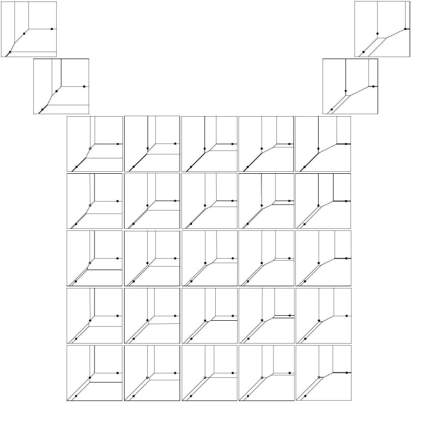
Figure 1. The plane $L_{X,Y,Z}$ of conics passing through three points $X,Y,Z\in{\mathbb{T}}{\mathbb{P}}^{2}$.

2. Two Points

Given two distinct points $x=(x_{0}{:}x_{1}{:}x_{2})$ and $y=(y_{0}{:}y_{1}{:}y_{2})$ in the projective plane $\mathbb{P}^{2}$ over a field $K$, there is a four-dimensional space $L_{x,y}$ of quadrics that vanish at $x$ and $y$, namely

(3) $$L_{x,y}\quad=\quad{\rm kernel}\begin{pmatrix}x_{0}^{2}&x_{1}^{2}&x_{2}^{2}&x_{0}x_{1}&x_{0}x_{2}&x_{1}x_{2}\\ y_{0}^{2}&y_{1}^{2}&y_{2}^{2}&y_{0}y_{1}&y_{0}y_{2}&y_{1}y_{2}\end{pmatrix}.$$

This defines a rational map which takes pairs of points into the Grassmannian:

$$\Psi\,:\,\mathbb{P}^{2}\times\mathbb{P}^{2}\,\longrightarrow\,{\rm Gr}(4,6)\subset\mathbb{P}^{14}$$

The map $\Psi$ blows up the diagonal in $\mathbb{P}^{2}{\times}\mathbb{P}^{2}$. The closure of its image is isomorphic to the Hilbert scheme of two points in $\mathbb{P}^{2}$. That is, $\,{\rm image}(\Psi)={\rm Hilb}_{2}(\mathbb{P}^{2})$ is a smooth $4$-dimensional subvariety of the $8$-dimensional Grassmannian ${\rm Gr}(4,6)$. Representing points in ${\rm Gr}(4,6)$ by their dual Plücker coordinates, the map $\Psi$ is given algebraically by evaluating the fifteen $2{\times}2$-minors of the matrix in (3). Gröbner-based implicitization of $\Psi$ yields the prime ideal

$$\begin{matrix}I_{2}=\!&\!\!\!\!\langle p_{03}p_{15}{+}p_{13}p_{34},p_{03}p_{24}{+}p_{04}p_{45},p_{03}p_{25}{+}p_{34}p_{45},p_{04}p_{13}{+}p_{03}p_{35},p_{04}p_{15}{-}p_{34}p_{35},p_{04}p_{25}{-}p_{24}p_{34},\\ &p_{13}p_{24}-p_{35}p_{45},p_{13}p_{25}-p_{15}p_{45},p_{15}p_{24}-p_{25}p_{35},\,p_{01}p_{02}-p_{05}^{2}+p_{34}^{2},p_{01}p_{12}+p_{14}^{2}-p_{35}^{2},\\ &p_{02}p_{12}-p_{23}^{2}+p_{45}^{2},\,p_{03}p_{23}-p_{34}^{2}+p_{04}p_{35},p_{04}p_{14}-p_{34}^{2}+p_{03}p_{45},p_{05}p_{15}-p_{35}^{2}-p_{13}p_{45},\\ &p_{05}p_{25}-p_{24}p_{35}-p_{45}^{2},\,p_{13}p_{23}+p_{14}p_{35}-p_{35}^{2}-p_{13}p_{45},\,p_{14}p_{24}-p_{24}p_{35}+p_{23}p_{45}-p_{45}^{2},\\ &\!\!\!\!\!p_{01}p_{04}{-}p_{03}p_{05}{-}p_{03}p_{34},p_{01}p_{23}{-}p_{14}p_{34}{+}p_{05}p_{35},p_{01}p_{24}{+}p_{05}p_{45}{+}p_{34}p_{45},p_{01}p_{25}{+}p_{14}p_{45}{+}p_{35}p_{45},\\ &\!\!\!\!\!p_{02}p_{03}{-}p_{04}p_{05}{+}p_{04}p_{34},p_{02}p_{13}{+}p_{05}p_{35}{-}p_{34}p_{35},p_{02}p_{14}{+}p_{23}p_{34}{+}p_{05}p_{45},p_{02}p_{15}{+}p_{23}p_{35}{+}p_{35}p_{45},\\ &\!\!\!\!\!p_{03}p_{12}{+}p_{14}p_{34}{-}p_{34}p_{35},p_{03}p_{14}{-}p_{01}p_{34}{+}p_{03}p_{35},p_{04}p_{12}{+}p_{23}p_{34}{-}p_{34}p_{45},p_{04}p_{23}{+}p_{02}p_{34}{+}p_{04}p_{45},\\ &\!\!\!\!\!p_{05}p_{12}{+}p_{23}p_{35}{-}p_{14}p_{45},p_{05}p_{13}{+}p_{13}p_{34}{+}p_{01}p_{35},p_{05}p_{14}{-}p_{34}p_{35}{+}p_{01}p_{45},p_{05}p_{23}{+}p_{02}p_{35}{+}p_{34}p_{45},\\ &\!\!\!\!\!p_{05}p_{24}{-}p_{24}p_{34}{+}p_{02}p_{45},p_{05}p_{34}{-}p_{04}p_{35}{+}p_{03}p_{45},p_{12}p_{13}{-}p_{14}p_{15}{+}p_{15}p_{35},p_{12}p_{24}{+}p_{23}p_{25}{-}p_{25}p_{45},\\ &\!\!\!\!\!p_{13}p_{14}{+}p_{01}p_{15}{+}p_{13}p_{35},p_{14}p_{23}{+}p_{12}p_{34}{-}p_{35}p_{45},p_{14}p_{25}{-}p_{25}p_{35}{-}p_{12}p_{45},p_{15}p_{23}{+}p_{12}p_{35}{-}p_{15}p_{45},\\ &\!\!\!\!\!p_{15}p_{34}{-}p_{14}p_{35}{+}p_{13}p_{45}\,,\,\,p_{23}p_{24}{+}p_{02}p_{25}{+}p_{24}p_{45}\,,\,\,p_{25}p_{34}{-}p_{24}p_{35}{+}p_{23}p_{45}\,\rangle.\end{matrix}$$

This is the ideal of the embedding of ${\rm Hilb}_{2}(\mathbb{P}^{2})$ via $\Psi$ as a subscheme of degree $21$ in $\mathbb{P}^{14}$.

We identify the tropicalization of ${\rm Gr}(4,6)$ with the space of tree metrics on six taxa [5, §2.4]. The taxa are the quadratic monomials. Combinatorially, this is a simplicial complex with $25$ vertices, $105$ edges and $105$ triangles. The $25$ vertices are the splits: trees with one internal edge. The tropicalization of $\Psi$ is a piecewise-linear map into that tree space:

$${\rm trop}(\Psi)\,:\,{\mathbb{T}}{\mathbb{P}}^{2}\times{\mathbb{T}}{\mathbb{P}}^{2}\,\longrightarrow\,{\rm trop}({\rm Gr}(4,6))\,\subset\,{\mathbb{T}}{\mathbb{P}}^{14}.$$

The coordinates of this map are the $15$ tropical $2{\times}2$-minors of the $2{\times}6$-matrix in (3):

$${\rm trop}(\Psi)(X,Y)\,=\,\bigl{(}{\rm max}(2X_{0}{+}2Y_{1},2X_{1}{+}2X_{0}),\ldots,{\rm max}(X_{0}{+}X_{2}{+}Y_{1}{+}Y_{2},X_{1}{+}X_{2}{+}Y_{0}{+}Y_{2})\bigr{)}.$$

We regard its image as a “combinatorial Hilbert scheme” that parametrizes pairs of points in ${\mathbb{T}}{\mathbb{P}}^{2}$ by the quadrics that pass through them. We have the following strict inclusions:

(4) $$\begin{matrix}&{\rm Hilb}_{2}({\mathbb{T}}{\mathbb{P}}^{2})&:=&{\rm image}({\rm trop}(\Psi))&&&\\ \,\subset\,&{\rm trop}({\rm Hilb}_{2}(\mathbb{P}^{2}))&=&{\rm trop}({\rm image}(\Psi))&\,\subset\,&{\rm trop}({\rm Gr}(4,6))&\,\subset\,&{\mathbb{T}}{\mathbb{P}}^{14}.\end{matrix}$$

Working modulo the common lineality spaces, the Hilbert schemes in (4) are one-dimensional complexes. These graphs are geometrically embedded, but not as subcomplexes, inside the two-dimensional simplicial complex $\,{\rm trop}({\rm Gr}(4,6))$. Alessandrini and Nesci argued in [1, §6.2] that ${\rm Hilb}_{2}({\mathbb{T}}{\mathbb{P}}^{2})$ is a cycle of length six. The following proposition extends their findings.

Proposition 2.1.

The tropicalized Hilbert scheme ${\rm trop}({\rm Hilb}_{2}(\mathbb{P}^{2}))$ is the graph with $16$ nodes and $30$ edges depicted in Figure 2. The outer $6$-cycle is the subgraph ${\rm Hilb}_{2}({\mathbb{T}}{\mathbb{P}}^{2})$. The labeling of the graph describes its embedding in the space of trees on six taxa and is explained below.

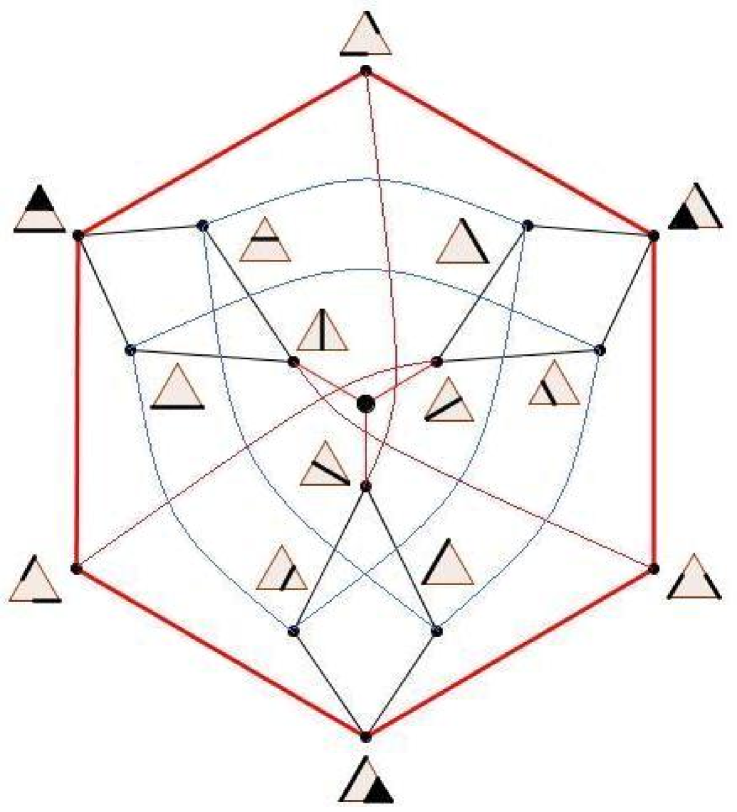
Figure 2. Tropicalization of the Hilbert scheme of two points in $\mathbb{P}^{2}$

We proved Proposition 2.1 by applying the software GFan [3] to the ideal $I_{2}$ and by carefully analyzing the output of that computation. We now discuss the outcome of that analysis.

The graph ${\rm trop}({\rm Hilb}_{2}(\mathbb{P}^{2}))$ has $16$ nodes. Twelve of the nodes are also nodes in the space of trees, ${\rm trop}({\rm Gr}(2,6))$, so they correspond to splits of the set of taxa $\{x_{0}^{2},x_{1}^{2},x_{2}^{2},x_{0}x_{1},x_{0}x_{2},x_{1}x_{2}\}$. Up to the action of the symmetric group $\mathfrak{S}_{3}$ by permuting the coordinates of $\mathbb{P}^{2}$, there are

1. three splits like $\,\{\,\{x_{0}^{2},x_{1}^{2}\}\,,\,\{x_{2}^{2},x_{0}x_{1},x_{0}x_{2},x_{1}x_{2}\}\,\}$,

2. three splits like $\,\{\,\{x_{0}^{2},x_{1}x_{2}\}\,,\,\{x_{1}^{2},x_{2}^{2},x_{0}x_{1},x_{0}x_{2}\}\,\}$,

3. three splits like $\,\{\,\{x_{0}x_{1},x_{0}x_{2}\}\,,\,\{x_{0}^{2},x_{1}^{2},x_{2}^{2},x_{1}x_{2}\}\,\}$,

4. three splits like $\,\{\,\{x_{0}^{2},x_{0}x_{1},x_{1}^{2}\}\,,\,\{x_{2}^{2},x_{0}x_{2},x_{1}x_{2}\}\,\}$.

The nine trees with one split in (1)-(3) have one cherry, or set of edges paired together. We represent that tree by drawing the cherry pair as a thick black segment in the corresponding vertex label of Figure 2. The three trees in (4) are 3-3 splits so they have no cherry. They appear alternatingly on the outer $6$-cycle in Figure 2, where they are drawn by a long segment across a triangle. The other three nodes on the outer $6$-cycle are trees with two interior nodes:

1. three split pairs like $\bigl{\{}\!\{\!\{x_{0}^{2},x_{0}x_{2}\}\!,\!\{x_{1}^{2},x_{2}^{2},x_{0}x_{1},x_{1}x_{2}\}\!\},\{\!\{x_{1}^{2},x_{1}x_{2}\}\!,\!\{x_{0}^{2},x_{2}^{2},x_{0}x_{1},x_{0}x_{2}\}\!\}\!\bigr{\}}$.

Finally, there is one special node that lies in the relative interior of a triangle in ${\rm trop}({\rm Gr}(2,6))$:

1. the unique trivalent snowflake tree with cherries $\{x_{0}^{2},x_{1}x_{2}\}$, $\{x_{1}^{2},x_{0}x_{2}\}$ and $\{x_{2}^{2},x_{0}x_{1}\}$.

The graph ${\rm trop}({\rm Hilb}_{2}(\mathbb{P}^{2}))$ has $30$ edges. Twelve are interior to triangles of ${\rm trop}({\rm Gr}(2,6))$, so they correspond to trivalent trees. Six of those are the edges of type (4-5) that form the outer $6$-cycle. The others are the three (2-6) edges adjacent to the snowflake tree, and the three (2-5) edges that appear as the longest edges in Figure 2. The remaining $18$ edges of ${\rm trop}({\rm Hilb}_{2}(\mathbb{P}^{2}))$ are also edges of ${\rm trop}({\rm Gr}(2,6))$, so they correspond to trees with two interior edges. Those edges are three (1-2)s, six (1-3)s, three (1-4)s, three (2-3)s, and three (3-4)s.

The tropical map ${\rm trop}(\Psi)$ amounts to a double cover of the $6$-cycle ${\rm Hilb}_{2}({\mathbb{T}}{\mathbb{P}}^{2})$. To see this, we note that the Newton polytope ${\rm NP}(\Psi)$ of the rational map $\Psi$, as defined in [5, (3.38)] is a centrally-symmetric $12$-gon. Namely, ${\rm NP}(\Psi)$ is the Minkowski sum of the $15$ Newton polytopes of all $2{\times}2$-minors of the $2{\times}6$-matrix (3), and these are line segments that lie in a common plane and involve six distinct directions. According to [5, Theorem 3.42], ${\rm trop}(\Psi)$ is linear on each of the twelve cones in the normal fan of ${\rm NP}(\Psi)$. The $12$-gon formed by these cones is mapped onto ${\rm Hilb}_{2}({\mathbb{T}}{\mathbb{P}}^{2})$ by looping twice around the outer $6$-gon in Figure 2.

3. Three Points

Guided by the above results for the two-point map $\Psi$, we now investigate the three-point map $\Phi$. We write $I_{3}$ for the homogeneous prime ideal that represents the image of $\Phi$. The following proposition summarizes basic facts about the variety $V(I_{3})={\rm image}(\Phi)\subset{\rm Gr}(3,6)$.

Proposition 3.1.

The projective variety $V(I_{3})$ has dimension $6$ and degree $57$. Its ideal $I_{3}$ is minimally generated by $62$ homogeneous quadrics in the $20$ Plücker coordinates $p_{ijk}$. Among these are $35$ quadrics that vanish on the Grassmannian ${\rm Gr}(3,6)\subset\mathbb{P}^{19}$. The corresponding tropical variety ${\rm trop}(V(I_{3}))$ in ${\mathbb{T}}{\mathbb{P}}^{19}$, with its Gröbner fan structure and taken modulo the lineality space, is a $3$-dimensional polyhedral complex with f-vector $(1095,6621,12830,7649)$.

Example 3.2.

The quadrics $\,p_{045}p_{145}-p_{013}p_{245}-p_{345}^{2}\,$ and $\,p_{025}p_{145}-p_{134}p_{245}-p_{015}p_{245}+p_{235}p_{345}\,$ are among the $27$ generators of the image of $I_{3}$ in the coordinate ring of ${\rm Gr}(3,6)$. ∎

There is a natural morphism from the Hilbert scheme ${\rm Hilb}_{3}(\mathbb{P}^{2})$ onto our variety $V(I_{3})$. However, unlike in Section 2, this is not an isomorphism. Geometrically, the morphism from the Hilbert scheme contracts all triples of points that lie on the same line. The singular locus of $V(I_{3})$ is a projective plane $\mathbb{P}^{2}$, namely, it is the image of all collinear triples in ${\rm Hilb}_{3}(\mathbb{P}^{2})$.

The Gröbner fan structure on the tropical variety in Propsition 3.1 is not simplicial: among the $7649$ three-dimensional polytopes, $876$ have five vertices ($105$ bipyramids and $773$ Egyptian pyraminds), $27$ have six vertices (all triangular prisms), and $12$ have seven vertices (two types). The number of $\mathfrak{S}_{3}$-orbits of facets of ${\rm trop}({\rm image}(\Phi))={\rm trop}(V(I_{3}))$ is $1318$.

Our results are summarized in Theorem 3.4. The role of the graph in Figure 2 is now played by the $3$-dimensional complex with $7649$ facets. It is obviously too big to be fully displayed here. Instead, we shall now focus on the leftmost complex in (2). The tropical morphism ${\rm trop}(\Phi)$ is a piecewise linear map. As shown in [5, §3.4], its domains of linearity are the normal cones of the Newton polytope. We begin by computing this Newton polytope.

Lemma 3.3.

The Newton polytope of $\Phi$ is $4$-dimensional and has f-vector $(504,1056,684,132)$.

The polytope ${\rm NP}(\Phi)$ plays the same role as the $12$-gon ${\rm NP}(\Psi)$ in Section 2. The $504$ vertices of ${\rm NP}(\Phi)$ correspond to distinct types of three labeled points in ${\mathbb{T}}{\mathbb{P}}^{2}$, where the type is the cell of ${\rm Trop}({\rm Gr}(3,6))$ that contains the plane of quadrics through these points. The map $\Phi$ is invariant under permuting the three points $x$, $y$ and $z$, and this reduces the number of image cones to $504/6=84$. These $84$ cones in ${\mathbb{T}}{\mathbb{P}}^{19}$ are grouped into $17$ orbits of size six with respect to the common symmetry group $\mathfrak{S}_{3}$ of $I_{3}$, $V(I_{3})$ and ${\rm Trop}(V(I_{3}))$. Those symmetries correspond to permuting the indices $0$, $1$ and $2$ of the coordinates on $\mathbb{P}^{2}$ or ${\mathbb{T}}{\mathbb{P}}^{2}$.

Table 1. The $17$ generic types of triples in ${\mathbb{T}}{\mathbb{P}}^{2}$ and their planes of conics

. Type Orbit Size Valency $(X_{1},X_{2})$ $(Y_{1},Y_{2})$ Plane $L_{X,Y,Z}$ 1 12 6 $(4,3)$ $(3,-1)$ FFFGG 2 36 5 $(6,5)$ $(3,-1)$ EFFG 3 36 5 $(4,5)$ $(2,-1)$ FFFGG 4 36 4 $(6,7)$ $(2,-1)$ EFFG 5 36 4 $(8,6)$ $(5,1)$ EFFG 6 36 4 $(5,8)$ $(-1,5)$ EEFG 7 36 4 $(5,6)$ $(2,1)$ EEFF(a) 8 36 4 $(3,7)$ $(-1,2)$ EEFG 9 36 4 $(6,5)$ $(4,2)$ EEFF(a) 10 36 4 $(5,6)$ $(3,1)$ EFFG 11 36 4 $(6,5)$ $(5,2)$ EFFG 12 36 4 $(4,6)$ $(2,3)$ EEFF(a) 13 12 4 $(5,3)$ $(3,-2)$ EEEG 14 18 4 $(3,6)$ $(1,3)$ EEFF(b) 15 18 4 $(3,6)$ $(2,3)$ EEFF(b) 16 36 4 $(3,5)$ $(2,1)$ EEFG 17 12 4 $(2,3)$ $(3,1)$ EEEG

Given three points $X=(X_{0},X_{1},X_{2})$, $Y=(Y_{0},Y_{1},Y_{2})$ and $Z=(Z_{0},Z_{1},Z_{2})$ in the tropical projective plane ${\mathbb{T}}{\mathbb{P}}^{2}$, we write $L_{X,Y,Z}$ for the tropical $2$-plane in ${\mathbb{T}}{\mathbb{P}}^{5}$ determined, as in [5, (3.44)] or [7, §2], by the tropical Plücker vector $\,{\rm trop}(\Phi)(X,Y,Z)\,\in\,{\rm trop}({\rm Gr}(3,6))\,\subset\,{\mathbb{T}}{\mathbb{P}}^{19}$. Geometrically, $L_{X,Y,Z}$ is the tropical plane whose points are the tropical quadrics that pass through the points $X,Y,Z$. Our picture of this in Figure 1 is reminiscent of [6, Fig. 19].

Our main result is the classification of the $17$ types of configurations of triples of points.

Theorem 3.4.

Precisely $48$ of the $1005$ generic $2$-planes in ${\mathbb{T}}{\mathbb{P}}^{5}$ arise as $L_{X,Y,Z}$ for some triple $X,Y,Z\in{\mathbb{T}}{\mathbb{P}}^{2}$. This covers six of the seven symmetry classes. Table 1 summarizes the correspondence between the $17$ types of triples and the $6$ combinatorial types of $2$-planes.

We proved this theorem by explicit computations. We shall explain our method and how to read Table 1. For each of the $17$, types we list a representative configuration. Here we break the symmetry by setting $X_{0}=Y_{0}=Z_{0}=0$ and by fixing the third point to lie at the origin, i.e. $Z=(Z_{1},Z_{2})=(0,0)$. For each configuration, the first point $X=(X_{1},X_{2})$ is listed in the fourth column, and the second point $Y=(Y_{1},Y_{2})$ is listed in the fifth column.

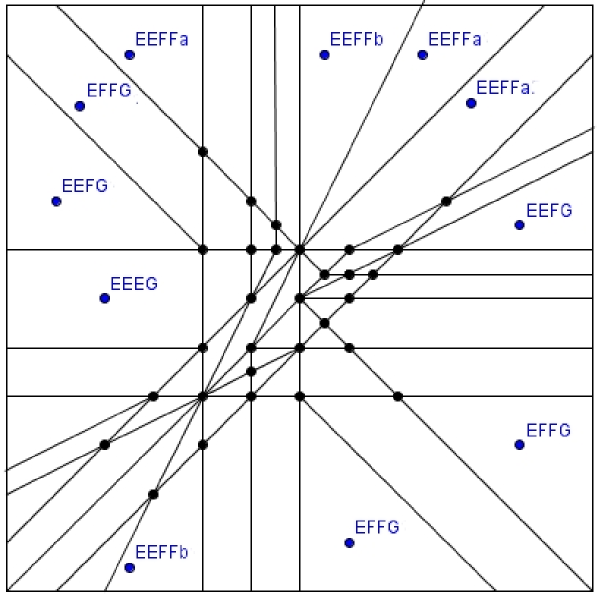
Figure 3. Partition of the $(Z_{1},Z_{2})$-plane obtained by $X=(0,0)$ and $Y=(2,3)$.

The second column, “Orbit Size”, lists of the cardinality of the orbit of the configuration under permuting both points and coordinates. The sum of the $17$ orbit sizes is $504$, the total number of vertices of ${\rm NP}(\Phi)$. The third column, “Valency”, lists the number of edges of the Newton polytope ${\rm NP}(\Phi)$ that are adjacent to the given vertex. Equivalently, this is the number of linear inequalities needed to characterize the configurations of the type in question. For instance, there are six such linear inequalities for type 1:

(5) $$X_{1}\geq X_{2},\,\,X_{1}\geq Y_{1},\,\,Y_{2}\leq 0,\,\,X_{2}+2Y_{1}\geq 2X_{1},\,\,2X_{2}+Y_{1}\geq 2X_{1},\,\,X_{2}+Y_{1}+Y_{2}\geq X_{1}.$$

One solution is $\{X=(4,3),Y=(3,-1)\}$. A solution is equivalent, in the sense that the plane $L_{X,Y,Z}$ is in the same maximal cone of ${\rm trop}({\rm Gr}(3,6))$, if and only if the six inequalities in (5) are satisfied. The solution set of (5) is the cone over a bipyramid. The corresponding vertex figure of ${\rm NP}(\Phi)$ is a cube. The vertex figures for types 2 and 3 are Egyptian pyramids. All other $14$ types of vertices are simple, so those vertex figures of ${\rm NP}(\Phi)$ are tetrahedra.

One way to visualize the partition of $\mathbb{R}^{4}$ into $504$ normal cones to ${\rm NP}(\Phi)$ is to intersect this normal fan with the $2$-dimensional affine space obtained by also fixing the second point $Y=(Y_{1},Y_{2})$ at a particular location. For instance, in Figure 3 we fix $Y=(2,3)$, and we allow $X=(X_{1},X_{2})$ to vary over the plane. The regions of equivalence are convex polygons. On each polygon, the plane of conics $L_{X,Y,Z}$ has a fixed combinatorial type in ${\rm trop}({\rm Gr}(3,6))$.

The tropicalization of ${\rm Gr}(3,6)$ has seven $\mathfrak{S}_{6}$-orbits of maximal cones. The interior of each corresponds to a distinct type of plane in ${\mathbb{T}}{\mathbb{P}}^{5}$. These types were classified in [8, §5] and given the names EEEE, EEFF(a), EEFF(b), EFFG, EEEG, EEFG, and FFFGG. See [2, Figure 1] for a diagram that shows these seven planes. In the last column of Table 1, we see that EEEE is the unique type that does not arise as $L_{X,Y,Z}$ for any triple $X,Y,Z$ in ${\mathbb{T}}{\mathbb{P}}^{2}$. The other six types arise as planes of conics through three points, as also seen in Figure 3.

Each tropical plane consists of bounded and unbounded faces. These are dual to the interior cells and boundary cells of a matroid subdivision of the second hypersimplex [7]. Each cell is indexed by a matroid of rank $3$ on the ground set $\{1,2,3,4,5,6\}$. Intersecting a generic tropical plane in ${\mathbb{T}}{\mathbb{P}}^{5}$ with the six tropical hyperplanes at infinity gives a tree arrangement consisting of six trees with five leaves each. A detailed description of the correspondence between tropical planes and tree arrangements is given in [2, §4]. For our planes $L_{X,Y,Z}$ that arise from triples $X,Y,Z\in{\mathbb{T}}{\mathbb{P}}^{2}$, we can construct the corresponding arrangement of six trees by removing in turn each of the six monomials $\{U_{0}^{2},U_{1}^{2},U_{2}^{2},U_{0}U_{1},U_{0}U_{2},U_{1}U_{2}\}$ from the defining equation of the conic. In other words, each of the six trees represents a line in ${\mathbb{T}}{\mathbb{P}}^{4}$. That line is a tree which parameterizes conics with five fixed terms that pass through the three given points. These trees are similar to [6, Fig. 19] but have only five taxa.

Now we explain how we constructed Table 1. We first computed the Newton polytope ${\rm NP}(\Phi)$ using Gfan, and we picked a representative in each maximal cone of its normal fan. Up to symmetries, these are the $17$ displayed configurations $X=(X_{1},X_{2}),Y=(Y_{1},Y_{2}),Z=(0,0)$. For these we calculated the corresponding vectors of tropical Plücker coordinates

$$({\rm trop}(\Phi))(X,Y,Z)\,\,=\,\,\bigl{(}P_{012},P_{013},P_{014},\ldots,P_{245},P_{345}\bigr{)}\,\,\in\,\,\mathbb{R}^{20}.$$

For each of the six indices, we consider the restricted vector of Plücker coordinates involving that index. For instance, for index “$0$”, corresponding to the monomial $U_{0}^{2}$, this is the vector

$$(P_{012},P_{013},P_{014},P_{023},P_{024},P_{034}).$$

This vector represents the pairwise distances in a phylogenetic tree with taxa $\{1,2,3,4,5\}$. This is the first among the six trees that represent the plane $L_{X,Y,Z}$, in its guise as a $3$-tree [5, (3.44)]. At this point, the last column in Table 1 can simply read off from [2, Table 2].

Acknowledgements. We are grateful to Anders Jensen for helping us with our Gfan computation. This work is based on the undergraduate senior thesis of the first author. The second author was partially supported by the NSF (DMS-0456960 and DMS-0757207).

References

- [1] D. Alessandrini and M. Nesci: On the tropicalization of the Hilbert scheme, arXiv:0912.0082.
- [2] S. Herrmann, A. Jensen, M. Joswig, and B. Sturmfels: How to draw tropical planes, Electron. J. Combin. 16 (2009) # 6.
- [3] A Jensen: Gfan, a Software System for Gröbner fans and tropical varieties, Available at http://www.math.tu-berlin.de/~jensen/software/gfan/gfan.html.
- [4] G. Mikhalkin: Tropical geometry and its applications. International Congress of Mathematicians. Vol. II, 827–852, Eur. Math. Soc., Zürich, 2006.
- [5] L. Pachter and B. Sturmfels: Algebraic Statistics for Computational Biology, Cambridge University Press, 2005.
- [6] J. Richter-Gebert, B. Sturmfels and T. Theobald: First steps in tropical geometry. Idempotent mathematics and mathematical physics, 289–317, Contemp. Math., 377, Amer.Math.Soc., Providence, 2005.
- [7] D. Speyer: Tropical linear spaces, SIAM J. Discrete Math. 22 (2008) 1527–1558.
- [8] D. Speyer and B. Sturmfels: The tropical Grassmannian, Advances in Geometry 4 (2004) 389–411.