Dissipational versus Dissipationless Galaxy Formation and the Dark Matter Content of Galaxies

Abstract

We examine two extreme models for the build-up of the stellar component of luminous elliptical galaxies. In one case, we assume the build-up of stars is dissipational, with centrally accreted gas radiating away its orbital and thermal energy; the dark matter halo will undergo adiabatic contraction and the central dark matter density profile will steepen. For the second model, we assume the central galaxy is assembled by a series of dissipationless mergers of stellar clumps that have formed far from the nascent galaxy. In order to be accreted, these clumps lose their orbital energy to the dark matter halo via dynamical friction, thereby heating the central dark matter and smoothing the dark matter density cusp. The central dark matter density profiles differ drastically between these models. For the isolated elliptical galaxy, NGC 4494, the central dark matter densities follow the power-laws $r^{-0.2}$ and $r^{-1.7}$ for the dissipational and dissipationless models, respectively. By matching the dissipational and dissipationless models to observations of the stellar component of elliptical galaxies, we examine the relative contributions of dissipational and dissipationless mergers to the formation of elliptical galaxies and look for observational tests that will distinguish between these models. Comparisons to strong lensing brightest cluster galaxies yield median $(M_{*}/L)_{B}$ ratios of $2.1\pm 0.8$ and $5.2\pm 1.7$ at $z\approx 0.39$ for the dissipational and dissipationless models, respectively. For NGC 4494, the best-fit dissipational and dissipationless models have $(M_{*}/L)_{B}=2.97$ and $3.96$. Comparisons to expected stellar mass-to-light ratios from passive evolution and population syntheses appear to rule out a purely dissipational formation mechanism for the central stellar regions of giant elliptical galaxies.

1. Introduction

How is the stellar content of galaxies assembled? Two extreme, contrasting models for the assembly of stars in galaxies have been considered over the years with no conclusive evidence as yet as to which mode dominates in which systems at which times. At one extreme, we can treat the process as totally dissipational with regard to energy; gas flows in from the virial radius, radiating away the kinetic and thermal energy it acquires while descending into the deep potential well of the dark matter halo. Once in place, the gas is transformed into stars ‘in situ’–in approximately the regions in which we see stars in fully-formed galaxies today. The other extreme model postulates that stars are formed in smaller stellar systems far outside the effective radius of the ultimate galaxy. From there, they lose orbital energy via dynamical friction and lose their potential energy only by heating or expelling other matter. These stars could be considered ‘accreted,’ whether by minor or major mergers. The balance between these two processes of galaxy formation (both of which surely occur) is unknown; determining that balance should help us to unravel some apparent paradoxes in the standard $\Lambda\mathrm{CDM}$ model of cosmology.

Although the $\Lambda\mathrm{CDM}$ model of cosmology has been very successful explaining large scale observations, such as the cosmic microwave background and the large scale structure of galaxies, it has not enjoyed as much success on smaller, galactic scales. One notable discrepancy between simply-modeled $\Lambda\mathrm{CDM}$ predictions and observations is the difference between the predicted and observed dark matter content in the centers of galaxies. Many N-body simulations of dark matter particles have been performed, and they show that cold dark matter will collapse into self-similar halos with a central density cusp (Fukushige & Makino 1997; Navarro et al. 1997; Moore et al. 1999; Diemand et al. 2005; Springel et al. 2008, but see). The steepness of the cusp may vary from $r^{-1}$ in the case of the NFW profile (Navarro et al. 1997) to as steep as $r^{-1.5}$ (Moore et al. 1999). Other studies (Subramanian et al. 2000; Ricotti 2003) have shown a range of central slope indices, $1<\alpha<1.5$ for $r^{-\alpha}$, depending on time, mass, and environment.

Cold dark matter simulations uniformly predict that dark matter halos should be universally cuspy, but observations have yet unambiguously to find these cusps. Indeed, observations of gravitational lensing, stellar velocity dispersions, and gas dynamics suggest inner dark matter density profiles are cored ($r^{\alpha}$, $\alpha>-1$) instead of cuspy (Flores & Primack 1994; Romanowsky et al. 2003; Swaters et al. 2003; Gentile et al. 2004; Sand et al. 2004; Simon et al. 2005; Cappellari et al. 2006; Gilmore et al. 2007; Gentile et al. 2007; de Blok et al. 2008; Oh et al. 2008; Napolitano et al. 2009; Rhee et al. 2004; Spekkens et al. 2005; Valenzuela et al. 2007, but see). For the Milky Way, it has been shown that within the errors of the microlensing observations, stars alone can more than account for the total mass density of the galaxy, leaving little room for a dark matter component in the center (Binney & Evans 2001).

Acceptance of both the dark matter simulations and the observations of dark matter density profiles leaves us with an apparent discrepancy. One way to solve this discrepancy is to abandon $\Lambda\mathrm{CDM}$. For example, the self-interactions of warm dark matter will smooth central density cusps (Spergel & Steinhardt 2000; Bode et al. 2001). Another solution to this discrepancy may lie in a misunderstanding of galaxy formation and the assembly of stellar material at the center of dark matter halos. The addition of baryons to dark matter halos can have a profound effect on the dark matter profile of a galaxy. One such effect is the adiabatic contraction of dark matter by the slow addition of baryons to the center of the potential well (Blumenthal et al. 1986). Adiabatic contraction has been observed in simulations with both dark matter and baryons (Navarro & Benz 1991; Navarro & White 1994; Jesseit et al. 2002; Abadi et al. 2003; Gnedin et al. 2004). This process conserves the adiabatic invariants of the dark matter orbits. With regard to energy, however, it is a dissipational process, as the orbital energy of the infalling baryonic material is radiated away and lost from the system. Because the dark matter density increases in the center of the galaxy under adiabatic contraction, the discrepancy between simulations and observations is only made worse, in the sense that the inner slope would be steeper than the NFW slope. For example, if the ultimate mass profile is “isothermal,” ($\rho_{\mathrm{tot}}(r)\propto r^{-2}$), then a dark matter profile with an initial slope index $1<\alpha<1.5$, ($r^{-\alpha}$), would have a post-adiabatic-contraction index of $1.67<\alpha<1.8$.

Processes which lower the dark matter density in the central regions of galaxies have also been explored. These processes are dissipationless; energy from stellar baryons is transferred to the dark matter, heating it and lowering the central dark matter density. Such processes include interactions of the dark matter with a stellar bar (Weinberg & Katz 2002; Holley-Bockelmann et al. 2005; McMillan & Dehnen 2005), baryon energy feedback from AGN(Peirani et al. 2008), decay of binary black hole orbits after galaxies merge (Milosavljević & Merritt 2001), scattering of dark matter particles by gravitational heating from infalling subhalos (Ma & Boylan-Kolchin 2004), and dynamical friction of stellar/dark matter clumps against the smooth background dark matter halo (El-Zant et al. 2001, 2004; Tonini et al. 2006; Romano-Díaz et al. 2008, 2009; Jardel & Sellwood 2009). In order to be successful, these methods must retain the strong central stellar concentration observed in large galaxies.

El-Zant et al. (2001) propose erasing the dark matter cusp via dynamical friction of incoming stellar/dark matter clumps against the dark matter background. Romano-Díaz et al. (2008) tested this hypothesis with dark matter/baryon N-body/SPH simulations and found that the introduction of baryons can flatten the dark matter cores in the inner 3 kpc. Romano-Díaz et al. (2008) claim that this cusp-flattening is not seen in other baryon/DM simulations because of a low numerical resolution and a focus on early, dissipational galaxy formation. Recent simulations (Naab et al. 2007; Abadi et al. 2009; Johansson et al. 2009) including both dark matter and baryons have shown similar departures from the standard adiabatic contraction model. In their cosmological simulations for building up elliptical galaxies, Johansson et al. (2009) note that their results show reasonably low dark matter fractions in the inner $10\ \mathrm{kpc}$ and that the assembly of their elliptical galaxies at late times is dominated by accretion of stellar lumps, not gas, which as noted above, tend to reduce the dark matter concentration. Similarly, accretion at late times has been invoked to erase the dark matter cusp formed by early adiabatic contraction, bringing dark matter halos to a universal (e.g. NFW) profile (Loeb & Peebles 2003; Gao et al. 2004).

Dynamical friction of stellar lumps against the dark matter halo represents a dissipationless method of stellar build-up in which the orbital energy of the infalling stars is transferred to the dark matter, thereby heating it and driving it out of the central parts of the galaxies. This is in direct contrast to the case of adiabatic contraction, which arises from a dissipational build-up of stellar material. Although both processes undoubtedly take place, the fully dissipational (adiabatic contraction) and fully dissipationless (dynamical friction) scenarios for galaxy formation represent the two extrema. Since these two processes have opposite effects on the central dark matter content of galaxies, the balance between them will determine the present-day dark matter density profiles in galaxies.

In this paper we explore the physics of galaxy assembly, presenting two toy models for the two extremes of galaxy formation constrained to produce the same observed final stellar distributions: one model for the fully dissipational build-up of stellar matter with star formation occurring in-situ and one model for the fully dissipationless build-up of stellar matter with stars added by accretion. The models are described in §2. We focus on the structure of giant elliptical galaxies whose light profiles are well-described by Sersic models. Taking the observed stellar profile of the galaxy as given, but leaving the stellar mass-to-light ratio, $M_{*}/L$, as a free parameter, we model the assembly of the stellar component via the two extreme formation methods. Then, by comparing the properties of the galaxies formed by these two methods to observations, we can begin to determine which method of assembling stars dominates and help to resolve the discrepancies between the simulated and observed dark matter density profiles.

Throughout this paper, we adopt the $\Lambda\mathrm{CDM}$ cosmology with $H_{0}=70\ \mathrm{h}_{70}\ \mathrm{km\ s}^{-1}$, $\Omega_{\mathrm{baryon}}/\Omega_{\mathrm{matter}}=0.17$, $\Omega_{\mathrm{matter}}=0.26$, and $\Omega_{\Lambda}=0.74$.

2. Models

In this section, we describe the two toy models of galaxy formation used in this paper. The first assumes that the orbital energy of the in-falling baryons is deposited entirely in the dark matter halo, while the second assumes energy is radiated away, leaving the galaxy-halo system.

In both models, we assume that both the dark matter and the baryonic matter follow circular orbits. For simplicity, we also assume the initial conditions (before the formation of the galaxy) for both the dark matter and the baryons are NFW density profiles, $\rho\propto[(r/r_{\mathrm{NFW}})(1+r/r_{\mathrm{NFW}})^{2}]^{-1}$, with the same concentrations. The ratio of baryon to dark matter density is equal to the universal fraction, which we assume to be $\Omega_{\mathrm{baryon}}/\Omega_{\mathrm{darkmatter}}=0.20$. In reality, the baryons will have a broader distribution than the dark matter, because the baryons are coupled to the radiation background. However, the additional thermal energy of the baryons corresponds to a velocity less than $10\ \mathrm{km\ s}^{-1}$, which is negligible for halos more massive than $\sim 10^{8}\ M_{\odot}$. In this study, we restrict ourselves to large halos, and can safely assume the baryons are initially distributed identically to the dark matter. We have verified this is a valid assumption by placing all the baryons initially outside the virial radius where they have negligible binding energy. This does not affect any of the results in this paper, altering the dark matter mass with $5\ {R_{\mathrm{e}}}$ by a few parts in $10^{3}$.

The final condition to which the models evolve is an elliptical galaxy with a predetermined stellar luminosity profile in the center of a dark matter halo. In both the dissipational and dissipationless models, we assume that the final galaxies contain no gas; all the baryons are accounted for in stars. This assumption is justified because the gas mass in elliptical galaxies today is usually only a few percent of the total baryon mass in these galaxies (Georgakakis et al. 2001).

For both models, the dark matter and stellar matter profiles are discretized into spherical shells such that the radius of a shell is at least two orders of magnitude larger than its width, and each shell is taken to be of homogeneous density. In order to form the galaxy, shells of stellar matter are moved inwards. Each time a shell of stellar matter passes through a shell of dark matter, the stars’ orbital energy is either deposited in the dark matter shell (dissipationless model) causing the dark matter shell to move outwards, or the stars’ orbital and thermal energy is radiated away causing the dark matter shell’s average radius to decrease as it undergoes adiabatic contraction. Since truly spherical shells would not suffer from dynamical friction, we are in fact considering a shell composed of stellar clumps, all of which (at any given time) have the same energy and angular momentum per unit mass, but whose angular momentum vectors are oriented randomly, giving the shell a total angular momentum of zero. Additionally, we assume that the stellar clumps do not contain any dark matter, as they formed far from the center of the dark matter halo, where the density is low. In reality, these clumps will contain some dark matter, much of which will be stripped before the stellar clump merges with the galaxy. Any remaining dark matter will undergo dynamical friction against the background dark matter. Because the system is spherically symmetric, a given dark matter shell is only affected by matter that crosses through it, but not by the rearrangement of matter interior or exterior to it. Therefore a procedure that describes a single shell crossing can be repeated many times for many shells, until the desired galaxy has been assembled.

2.1. Dissipationless Model: Dynamical Friction

In the dissipationless model, all the orbital energy lost by the stars in forming the galaxy is deposited in the dark matter halo. In this case, the galaxy is built up by ‘dry,’ dissipationless mergers.

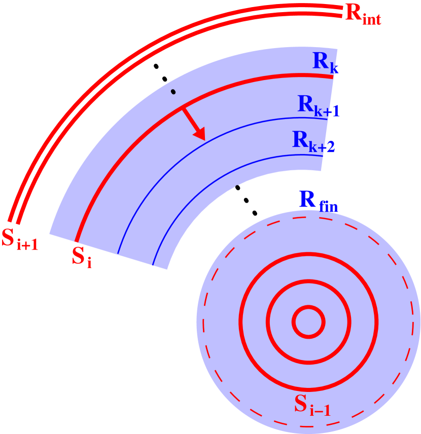
We imagine constructing the Sersic profile of the stars in a shell by shell fashion, sequentially moving each shell of stars from a large radius to its final position, in such a way that two stellar shells never cross. Therefore, the problem can first be idealized as moving one infinitely thin stellar shell from a large radius $R_{\mathrm{i}}$ to a smaller, final radius $R_{\mathrm{fin}}$. As the stellar shell moves, it passes through a dark matter distribution with a mass distribution $M_{\mathrm{dark}}(r)$, to which the stellar shell gives its orbital energy. The dark matter can be subdivided into a series of mass shells of thickness $\Delta R_{k}$, such that $\sum_{k}\Delta R_{k}=R_{\mathrm{int}}-R_{\mathrm{fin}}$. Therefore, we only need to compute the effects of one stellar shell passing through one dark matter shell uniformly distributed between $R_{k}$ and $R_{k+1}$, with thickness $\Delta R_{k}$, and then execute a double sum over the dark matter shells and all the stellar shells. A depiction of this process is shown in Figure 1. In the figure, the sum over dark matter shells is indexed by $k$, while the sum over the stellar shells is indexed by $i$.

Figure 1.— A cartoon depiction of the process by which we move stellar shells in to form a galaxy. The thin stellar shells are shown in red and labeled by $S_{i}$. The dark matter background is shown in blue and discretized into layers of uniform density and width $R_{k}-R_{k+1}$. The stellar shell $S_{i}$ is being moved from $R_{k}$ to $R_{k+1}$ as shown by the arrow.

The total energy lost by a single stellar shell as it moves from $R_{k}$ to $R_{k+1}$ can be calculated by taking the difference between the energy change of the stellar shell as it moves from a large initial radius, $R_{\mathrm{int}}$, with zero potential and zero kinetic energy, to $R_{k+1}$ and the energy change as it moves from $R_{\mathrm{int}}$ to $R_{k}$. The changes in kinetic and potential energy per unit mass of the stellar shell as it moves from $R_{\mathrm{int}}$ to $R_{k}$ are

$$\Delta T_{k} = \frac{1}{2}\frac{\mathrm{G}M(R_{k})}{R_{k}}\,,\qquad\mathrm{and}$$ (1)

$$\Delta W_{k} = -\frac{\mathrm{G}M(R_{k})}{R_{k}}-\int_{R_{k}}^{R_{\mathrm{int}}}\frac{\mathrm{G}\,\mathrm{d}M_{\mathrm{dark}}(r)}{r}\,,$$ (2)

where $M(r)$ includes both the dark matter and any stellar matter interior to $r$. By assumption, there is no stellar matter between $R_{\mathrm{int}}$ and $R_{k}$, so the integral in the potential energy depends only on $M_{\mathrm{dark}}$. The change in total energy of the stellar shell as it moves from $R_{k}$ to $R_{k+1}$ is thus

$$\Delta E_{k} = \frac{\mathrm{G}M_{\mathrm{dark}}(R_{k})}{2R_{k}}-\frac{\mathrm{G}M_{\mathrm{dark}}(R_{k+1})}{2R_{k+1}}+$$

$$\,\frac{\mathrm{G}M_{\mathrm{star}}(R_{k})}{2}\left(\frac{1}{R_{k+1}}-\frac{1}{R_{k}}\right)+$$

$$\,\int_{R_{k}}^{R_{k+1}}\frac{\mathrm{G}\,\mathrm{d}M_{\mathrm{dark}}(r)}{r}\,.$$

The stellar shell is made of up of small lumps of stars that will undergo dynamical friction against the dark matter background as they move; the energy lost by the stars as they move from $R_{k}$ to $R_{k+1}$ must be deposited in the dark matter. We assume that the exchange of energy between stars and dark matter is a local process. Therefore, all the energy of the stars is deposited in the dark matter initially orbiting between $R_{k}$ and $R_{k+1}$. As the dark matter gains energy, it’s orbit will expand, and the uniform density dark matter shell between $R_{k}$ and $R_{k+1}$ will become wider. Since we are assuming the energy exchange is local, the dark matter orbiting at the inner radius ($R_{k+1}$) will not move. In reality, this dark matter is affected by both adiabatic contraction, since the stars add mass interior to $R_{k+1}$, and dynamical friction, since the energy exchange is not purely local; this layer will move, but the movement will be second order in $\Delta R_{k}=R_{k}-R_{k+1}$. Therefore, by conserving energy the only quantity which changes is thickness of the dark matter shell the stars have moved through and consequently its mean radius.

In order to calculate the new dark matter layer thickness, we repeat the procedure above, but this time also account for the energy of the dark matter shell both before and after the stars move through it. As above, we assume a spherical dark matter shell of mass $M_{\mathrm{DM}}$ and uniform density, with an inner radius of $R$ (corresponding to $R_{k+1}$ above), and a thickness $\Delta R<<R$. Directly exterior to the dark matter shell is an infinitesimally thin stellar shell of mass $\Delta M_{*}$, at the radius $R+\Delta R$. The kinetic+potential energy of the two-shell system can be broken into the self-interaction energy of the dark matter shell, $E_{\mathrm{d}}$, the self-interaction energy of the stellar shell, $E_{\mathrm{s}}$, and the interaction energy of the two shells, $E_{\mathrm{ds}}$. To first order in $\Delta R$, these are given by:

$$E_{\mathrm{d}} = -\frac{\mathrm{G}M_{\mathrm{DM}}^{2}}{4R}\left(1-\frac{2}{3}\frac{\Delta R}{R}\right)\,;$$ (4)

$$E_{\mathrm{s}} = -\frac{\mathrm{G}\Delta M_{*}^{2}}{4R}\left(1-\frac{\Delta R}{R}\right)\,;$$ (5)

$$E_{\mathrm{ds}} = -\frac{\mathrm{G}\Delta M_{*}M_{\mathrm{DM}}}{2R}\left(1-\frac{\Delta R}{R}\right)\,.$$ (6)

The shells are embedded in a spherically symmetric galaxy which also contributes to the energy. We assume that the mass distribution of the galaxy remains fixed as the shells interact. This assumption is exactly true for the mass interior to the shells and the mass far outside the shells. We define $M_{\mathrm{int}}$ to be the total mass (dark matter $+$ baryons ) interior to $R$. This mass contributes kinetic+potential energy $E_{\mathrm{int}}$ to the shells while the mass external to $R+\Delta R$ contributes a potential energy $E_{\mathrm{ext}}$. These energies are given by

$$E_{\mathrm{int}} = -\frac{\mathrm{G}M_{\mathrm{int}}}{2R}\bigg{[}M_{\mathrm{DM}}\left(1-\frac{\Delta R}{2R}\right)+$$

$$\qquad\qquad\left.\Delta M_{*}\left(1-\frac{\Delta R}{R}\right)\right]\,,\ \quad\mathrm{and}$$

$$E_{\mathrm{ext}} = -\mathrm{G}\left(\Delta M_{*}+M_{\mathrm{DM}}\right)\int_{R+\Delta R}^{\infty}\frac{\mathrm{d}\,M(r)}{r}\,.$$ (8)

Therefore, the total initial energy of the two shells is given by the sum of equations (4)-(8).

We now move the stellar shell through the dark matter shell until the stellar shell is orbiting at the radius $R$, as in the above example. This time, however, we will include the changes in the dark matter distribution in the energy difference. After the move, the dark matter shell will widen from $\Delta R$ to $\Delta R^{\prime}$. Because $\Delta R^{\prime}$ is still small compared to $R$, the density of the dark matter layer is still uniform after the move. The final total energy of the stellar and dark matter shells after moving the stars is

$$E = -\frac{G}{2R}\bigg{[}\frac{M_{\mathrm{DM}}^{2}}{2}\left(1-\frac{2}{3}\frac{\Delta R^{\prime}}{R}\right)+\frac{\Delta M_{*}^{2}}{2}+$$

$$\qquad\Delta M_{*}M_{\mathrm{DM}}\left(1-\frac{\Delta R^{\prime}}{2R}\right)+$$

$$\qquad M_{\mathrm{int}}\left(M_{\mathrm{DM}}\left(1-\frac{\Delta R^{\prime}}{2R}\right)+\Delta M_{*}\right)\bigg{]}$$

$$-\mathrm{G}\left(\Delta M_{*}+M_{\mathrm{DM}}\right)\int_{R+\Delta R}^{\infty}\frac{\mathrm{d}\,M(r)}{r}+\Delta E_{\mathrm{ext}}\,.$$

If we assume that the mass initially exterior to $R+\Delta R$ is unaffected by the dark matter expanding to $R+\Delta R^{\prime}$, the change in external energy, $\Delta E_{\mathrm{ext}}$, depends only on the mass initially between $R+\Delta R$ and $R+\Delta R^{\prime}$, and the dark matter that moves beyond $R+\Delta R$. This assumption is valid to first order in $\Delta R$. Since both $\Delta R$ and $\Delta R^{\prime}$ are small compared to $R$, we assume that mass between $R+\Delta R$ and $R+\Delta R^{\prime}$ is of homogeneous density and a total mass $M_{\mathrm{ext}}$. Therefore,

$$\Delta E_{\mathrm{ext}}=\frac{\mathrm{G}M_{\mathrm{DM}}M_{\mathrm{ext}}}{4R}\frac{\Delta R^{\prime}-\Delta R}{\Delta R^{\prime}}\,.$$ (10)

Substituting this into equation 2.1 and taking the difference between the total energy of the two shells before and after the move yields

$$\Delta E = \frac{\mathrm{G}}{12R^{2}}\Bigg{\{}\left(\Delta R^{\prime}-\Delta R\right)M_{\mathrm{DM}}\bigg{[}2M_{\mathrm{DM}}+$$

$$\qquad\qquad\qquad 3\left(M_{\mathrm{int}}+\Delta M_{*}+\frac{R}{\Delta R^{\prime}}M_{\mathrm{ext}}\right)\bigg{]}-$$

$$\qquad\qquad 3\Delta R\Delta M_{*}\left(M_{\mathrm{DM}}+2M_{\mathrm{int}}+\Delta M_{*}\right)\Bigg{\}}\,.$$

This can be solved numerically for $\Delta R^{\prime}$, keeping in mind that $M_{\mathrm{ext}}$ is a function of $\Delta R^{\prime}$. In the limit that $M_{\mathrm{ext}}\to 0$, equation 2.1 can be solved analytically for $\Delta R^{\prime}$:

$$\frac{\Delta R^{\prime}}{\Delta R} = \frac{1/2M_{\mathrm{int}}+1/3M_{\mathrm{DM}}+3\Delta M_{*}}{1/2M_{\mathrm{int}}+1/3M_{\mathrm{DM}}+3/2\Delta M_{*}}+$$

$$\quad\frac{(\Delta M_{*}/M_{\mathrm{DM}})(M_{\mathrm{int}}+1/2\Delta M_{*})}{1/2M_{\mathrm{int}}+1/3M_{\mathrm{DM}}+3/2\Delta M_{*}}\,.$$

In the limit that $\Delta M_{*}<<M_{\mathrm{DM}}$ the ratio of widths goes to $1$ as expected. This procedure can be easily scaled up to a series of interleaved dark matter and stellar shells. As the stellar shells move inwards to form a galaxy, they expand each dark matter shell they cross, thereby slowly moving dark matter outward.

In the example above, all the energy from the stars is deposited in the dark matter layer which the stars cross. In our numerical calculations, the stars deposit their energy in a set of layers surrounding the layer they cross. The width of this set is proportional to the current radius and the amount of energy deposited in each layer is proportional to the mass of that layer. This approximates the wake created by infalling stellar material, which is responsible for the forces causing dynamical friction (Weinberg 1986). The size of the wake scales as $\mathrm{G}\Delta M_{*}/\sigma_{\mathrm{dm}}^{2}\approx(\Delta M_{*}/M_{\mathrm{int}})R$. We assume that the stars are added by a series of minor mergers, in which each added stellar shell of mass $\Delta M_{*}$ constitutes a minor merger. The mass ratio of such mergers is approximately $(\Delta M_{*}/M_{\mathrm{int}})\approx 1/10$, thus setting the size of the wake.

In a more accurate treatment, there would also be a diffusive term; each dark matter shell would spread out in radius as it was on average moved outwards when passed by a stellar shell.

In the calculations above, we assume no stellar shells cross each other. This is equivalent to assuming all the infalling material remains on spherical orbits. This is not true in reality, especially since galaxies are not spherical but often triaxial systems, which do not allow purely circular orbits as assumed above. If we allowed for triaxial systems in our models and allowed for the accretion of material on radial orbits, the infalling stars would deposit energy interior and exterior to their final mean orbital radius. This would have an effect on the final dark matter density profile, but the effect would depend on the fraction of energy deposited interior and exterior to the final orbital radius. If all the energy is deposited interior to the final orbital radius, then more dark matter would be displaced from the center, leading to a lower central dark matter density. The opposite is true if the energy is deposited outside the final orbital radius.

Additionally, if we relax the requirement that no stellar shells cross, we must take into account energy deposited in the stars, not just the dark matter. This will expand the stellar orbits, in the same way the dark matter orbits are expanded, and lower the stellar density in the center of the galaxy in the same way the dark matter density is lowered. Therefore, in order to make a galaxy with a given stellar density, we would first have to make a more concentrated stellar system, and then add stellar clumps which would undergo dynamical friction against the highly concentrated stellar system, thereby lowering the central stellar density to the desired value. Indeed, observations have been made of highly concentrated stellar systems at higher redshift (van Dokkum et al. 2008; Cappellari et al. 2009). In order to make highly concentrated stellar systems, the galaxies would have to undergo an early period of dissipational formation. This would also increase the central dark matter density before the onset of dissipationless formation, making the final dark matter density dependent on the relative importance of dissipational and dissipationless formation mechanisms. Simulations show that early type galaxy formation can be divided into two phases, an initial dissipational formation of a centrally concentrated system, followed by accretion via ‘dry’ mergers of additional stellar material (Naab et al. 2007, 2009; Cook et al. 2009). If we allowed stellar shell crossing, we would have to take into account the two phase growth of galaxies and combine the dissipational and dissipationless models into a single model. This work attempts to determine the relative importance of the dissipational and dissipationless formation mechanisms; we are only concerned with the two extreme formation models, which can be easily modeled assuming spherical galaxies and infalling material on circular orbits. The effects of triaxiality and radial orbits would require combining the dissipational and dissipationless formation mechanisms, which is left for future work.

Of course, dynamical friction on incoming stellar clumps is intrinsically a three-dimensional process (Tremaine & Weinberg 1984; Pichon & Aubert 2006; Aubert & Pichon 2007), and the treatment in spherical shells above is not intended to accurately mimic the actual assembly of a galaxy via dynamical friction. Rather, the adopted model is designed to be correct with respect to the total energy deposited in the dark matter. In the numerical calculations presented below, the total binding energy is conserved. As the width of the stellar shells decreases, the calculations conserve energy to approximately one part in $10^{5}$ of the binding energy of the stars in the final galaxy.

2.2. Dissipational Model: Adiabatic Contraction

For the dissipational build-up of galaxies we present the following picture: baryons in the form of gas slowly fall into the centers of dark matter potential wells, where the gas condenses to form stars. In this case, the gas radiates away its orbital and thermal energy as it falls inwards, so the total energy of the system is not conserved. However, as long as the gas is accreted into the center of the galaxy on a timescale that is long compared to the local dynamical time, the adiabatic invariants of the dark matter orbits will be conserved. In our model for adiabatic contraction, we follow the prescription of Blumenthal et al. (1986) and again assume circular orbits for the dark matter and a spherically symmetric mass distribution. Instead of energy being conserved, the adiabatic invariants of the dark matter orbits are conserved. For periodic orbits, $\oint\,p\mathrm{d}q$ is an adiabatic invariant, where $q$ is a coordinate and $p$ is its conjugate momentum. For a particle in a circular orbit at a radius $r$ around a spherical mass distribution $M(r)$, we take the conjugate momentum to be the angular momentum and its corresponding coordinate, the angular position. The adiabatic invariant is then:

$$J^{2}=\Big{(}\oint\,\sqrt{M(r)r}\mathrm{d}\theta\Big{)}\propto rM(r)\,.$$ (13)

Therefore, if the mass interior to the orbit, $M(r)$, increases, the orbital radius must decrease. Following the same set-up as in the previous model, we start with a dark matter shell of constant density and mass $M_{\mathrm{DM}}$ directly interior to an infinitesimally thin shell of stars/gas of mass $\Delta M_{*}$. After the baryons move interior to the dark matter layer, the inner radius of the dark matter shell becomes $R^{\prime}=R\,M_{\mathrm{int}}/(M_{\mathrm{int}}+\Delta M_{*})$ and the width of the layer becomes

$$\Delta R^{\prime}=\frac{(M_{\mathrm{int}}+M_{\mathrm{DM}})(R+\Delta R)}{M_{\mathrm{int}}+M_{\mathrm{DM}}+\Delta M_{*}}-R^{\prime}\,.$$ (14)

Overall, the dark matter shell moves inwards and becomes thicker or thinner depending on the mass ratios of the dark matter shell, the baryon shell, and the mass interior to both. As in the previous model, two shells only interact when their orbits cross, so this prescription for interchanging two shells can be scaled up to many shells.

If the constraint of circular orbits is removed, the adiabatic invariant is no longer $rM(r)$. Using N-body simulations, Gnedin et al. (2004) show that $M(\bar{r})r$, where $\bar{r}$ is the orbit-averaged position, is a good proxy for the adiabatic invariant. If this quantity is conserved for isotropic orbits, the prescription for adiabatic contraction remains the same. However, the prescription above will overestimate the amount of adiabatic contraction if the orbits are radially biased (Gnedin et al. 2004).

2.3. Models Fit to Example of Massive Galaxy

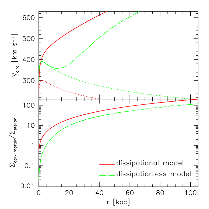
The difference in the dark matter density in the central regions of a galaxy for each model is clearly shown by the comparison of the velocity profiles of model galaxies. In the top panel of Figure 2, the circular velocity curves for both models are compared to the velocity curve produced by the stars alone. The models shown in Figure 2 are taken to fit very massive galaxies and we have adjusted $M_{*}/L$ such that the central velocity dispersions of both models are the same. The central velocity dispersions are computed assuming the stars are on isotropic orbits. In both cases, the stars dominate in the very central regions, but the differences in dark matter significantly affect both curves. The lower panel of Figure 2 shows the ratio of the dark matter to stellar matter projected densities as a function of radius for both models. In reality, since galaxies certainly form by a combination of dissipational and dissipationless methods, the velocity curves and the dark matter to stellar matter density ratios will fall somewhere in between the two extreme toy models examined here.

Figure 2.— The circular velocity (top) and projected dark matter to stellar density ratio (bottom) for an extremely massive $L=6.0\ L_{*}$ ($K$-band) galaxy in a $3.84\times 10^{14}\ M_{\odot}$ halo. The Sersic index is $n=6.80$ and the half light radius is 45.79 kpc. The stellar mass-to light ratios of the models are set to the values shown in the lower panel of Figure 3, such that the two models have the same central velocity dispersion ($\sigma_{0}\approx 270\ \mathrm{km\ s}^{-1}$). The solid line is for the dissipational model. The dashed line is for the dissipationless model. In the upper plot, the upper (dissipationless) and lower (dissipational) dotted lines are the circular velocity curves due to the stars alone.

In order to compute the two models, we require a set of input parameters describing the initial matter distribution and the final stellar distribution. If we assume the initial distribution of both components fit a single NFW profile, then the two required input parameters are the total mass of the halo and the initial concentration. Assuming that the galaxy is spherically symmetric, the final stellar mass distribution is completely described by the surface brightness profile of the galaxy and a stellar mass-light ratio. The luminosity profile can be directly observed and $M_{*}/L$ can be determined from observations of the central velocity dispersions of galaxies. Since stars dominate the mass in the central regions, they also are the dominant contribution to the central velocity dispersion. Thus, the observational input parameters for these models are the total luminosity of the galaxy, the luminosity profile (in the case of Sersic profiles, the necessary terms are the Sersic index, $n$, and the half-light (effective) radius, ${R_{\mathrm{e}}}$), and the central velocity dispersion. The free parameters are the total halo mass, the initial NFW concentration, and the stellar mass-to-light ratio (which we assume to be constant throughout a given system). Therefore, for a given galaxy, the two models will by construction have the same luminosity and central velocity dispersion, but the total halo masses and the mass-to-light ratios will be different, and in some cases, outside the bounds set by other observational and model constraints. Table 1 gives the parameters for the dissipational and dissipationless models which best fit the strong lensing cluster MS-2137-23 discussed in §3.4.

2.4. Minimum Radius for Galaxies Formed by Dissipationless Mergers

In order for a galaxy to form by purely dissipationless processes, the incoming stars must deposit their orbital energy in the dark matter halo. Therefore, the dark matter halo must initially have sufficient binding energy to give to the infalling stars. The stars in the final galaxy can have no more binding energy than the initial dark matter halo. This sets a lower limit on the size of a galaxy formed by purely dissipationless processes. A galaxy formed by dissipationless accretion would approach the minimum size and would have very little dark matter in the center, which is in agreement with observations mentioned in §1. However, if dissipational processes play a dominant role in galaxy formation, there is no minimum size for galaxies, as the infalling baryons can dissipate all of their orbital and thermal energy.

Given a cluster mass, concentration, and final galaxy stellar mass, and Sersic index, a lower limit on the galaxy’s effective radius, ${R_{\mathrm{e}}}$, can be obtained by setting the change in binding energy of the dark matter halo equal to change in binding energy of the stars and baryons in the cluster. For galaxies with $L\approx 10^{11}\ L_{\odot}$ in the $K$-band, the minimum effective radius for a dissipationlessly formed galaxy yields a reasonable minimum for the effective radius of observed early type galaxies. (Bernardi et al. 2003).

We should note that there is another limiting radius for the formation of accreted halos. A satellite may be destroyed by tidal shocks before it reaches the energetically allowed minimum radius, thereby depositing stars in the outer region of the growing galaxy (Kormendy 1977; Gnedin et al. 1999; Wetzel & White 2009). This process is difficult to compute but gives a limiting radius comparable to the dynamical friction limits computed above. For the most massive systems (BCGs), the tidal shock limiting radius is more severe than the dynamical friction one, so we can expect that the dark matter to stellar matter ratio in such systems will be higher than in more moderate mass galaxies.

3. Comparisons to Observations of BCGs

One test of the dissipational and dissipationless models of galaxy formation is the build-up of brightest cluster galaxies (BCGs). BCGs offer a good comparison sample for these spherically symmetric test models for several reasons. First, BCGs almost always sit at or nearly at the center of their host cluster. Therefore, they are also centered in a dark matter halo, so there are no contributions to the potential from an off-center halo, not included in our models. Furthermore, BCGs represent a uniform sample, so much so that they have been suggested as standard candles (Postman & Lauer 1995), allowing comparisons to be made to the entire population instead of individual galaxies. Finally, BCGs are thought to have been formed by a series of galaxy mergers during the build-up of clusters (Ostriker & Hausman 1977; Nipoti et al. 2004; Cooray & Milosavljević 2005), making them good candidate systems in which to observe dissipationless galaxy formation.

3.1. Scaling Relations for Input Parameters

In order to compare the models to observations, we normalize the models to $K$-band and $r$-band data of BCGs. Given the luminosity of a BCG and choosing a constant stellar mass-to-light ratio for the models, we use empirical relations to derive the cluster and the BCG properties. From Lin & Mohr (2004), the cluster mass is related to the observed $K$-band BCG luminosity by

$$\frac{L_{\mathrm{BCG}}}{10^{11}\mathrm{h}_{70}^{-2}\ L_{\odot}}=\left(4.9\pm 0.2\right)\left(\frac{M_{\mathrm{cluster}}}{10^{14}\ M_{\odot}}\right)^{0.26\pm 0.04}\,.$$ (15)

The luminosities of BCGs are 6-10 times brighter than $\mathrm{L}_{*}$ in the $K$-band. For galaxies typically in clusters, $M_{K*}=-24.34$ (Lin & Mohr 2004), including the BCG, or about $1.16\times 10^{11}\ L_{\odot}$ in the $K$-band. From the cluster mass, the cluster virial radius, $r_{200}$, can be calculated assuming the critical density $\rho_{\mathrm{cr}}=1.36\ \mathrm{h}_{70}^{2}\times 10^{11}\ M_{\odot}\ \mathrm{Mpc}^{-3}$. Simulations have shown that the dark matter halo concentration, $c=r_{\mathrm{200}}/r_{\mathrm{NFW}}$, scales approximately with the mass as (Neto et al. 2007)

$$c=4.67\left(\frac{M_{\mathrm{cluster}}}{10^{14}\ M_{\odot}}\right)^{-0.11}\,.$$ (16)

Equations 15 and 16 set the initial conditions for the models. The properties of the stellar component of the BCG can also be derived from $L_{\mathrm{BCG}}$. We assume that the BCGs are well-modeled by a single Sersic profile ($\mathrm{I}(R)\sim\exp(R^{1/n}),$ Sersic 1968), ignoring the ICL and outer components of the BCG (see Gonzalez et al. 2005). The two-dimensional surface brightness profile defined by Sersic can be deprojected numerically into a three-dimensional luminosity density profile, assuming the galaxy is spherically symmetric. This numerical deprojection is well-approximated by the analytic formula (Lima Neto et al. 1999):

$$\rho_{*}(r) \propto (r/{R_{\mathrm{e}}})^{1-1.188/(2n)+0.22/(4n^{2})}$$ (17)

$$\exp\left((0.327-2n)(r/{R_{\mathrm{e}}})^{1/n}\right)\,,$$

where $n$ is the Sersic index ($n=4$ for a de Vaucouleurs profile), and ${R_{\mathrm{e}}}$ is the half-light radius of the surface brightness profile. Observations show that the Sersic properties of BCGs are correlated with the galaxy’s luminosity. Using data from Lin & Mohr (2004) and Graham et al. (1996), the luminosity can be related to the half-light radius and the Sersic index by

$$\log{R_{\mathrm{e}}} = -10.30+1.01\log\left(\frac{L_{\mathrm{BCG}}}{L_{\odot}}\right)\quad\mathrm{and}$$ (18)

$$n = 2.9\log{R_{\mathrm{e}}}+1.98\,,$$ (19)

which are in good agreement with scaling relations from Vale & Ostriker (2008), Bernardi et al. (2007) and Desroches et al. (2007).

Also modeled in each galaxy is a central supermassive black hole, which adds a minor correction to the velocity dispersion of the galaxy. The black hole mass is determined from the galaxy luminosity by the relation (Graham 2007):

$$\log\left(\frac{M_{\mathrm{BH}}}{M_{\odot}}\right)=$$ (20)

$$\quad(0.95\pm 0.15)\log\left(\frac{L_{\mathrm{BCG}}}{10^{10.91}\ L_{\odot}{}_{\mathrm{,}K}}\right)+(8.26\pm 0.11)\,.$$

Thus, by supplying a galaxy luminosity and a stellar mass-to-light ratio, we can obtain all the other input parameters needed to compare the dissipational and dissipationless models to observations of BCGs.

3.2. The $L$–$\sigma$ Relation

The innermost probe of the mass profile is the central velocity dispersion of a galaxy. Elliptical galaxies fall on the fundamental plane (Djorgovski & Davis 1987; Dressler et al. 1987) and one projection of the plane is the Faber-Jackson relation: the relation between a galaxy’s luminosity, $L$, and velocity dispersion, $\sigma$ (Faber & Jackson 1976). In the $K$-band, the Faber-Jackson relation observed by Pahre et al. (1998) is

$$M_{K}=-10.35\pm 0.55\log\sigma_{0}\,.$$ (21)

For BCGs, Lauer et al. (2007) show that the velocity dispersion saturates at high luminosities, leading to the relation

$$M_{V}=-2.5(6.5\pm 1.3)\log\left(\frac{\sigma}{250\ \mathrm{km\ s}^{-1}}\right)-22.45\pm 0.18\,.$$ (22)

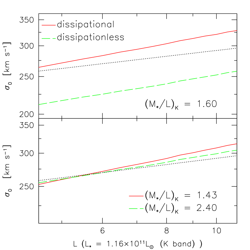
Desroches et al. (2007) find a similar relation. In order to compare to the $L$–$\sigma$ relation for BCGs, we normalize our models to observed BCGs using the scaling relations described in §3.1. The line-of-sight central velocity dispersions averaged over an aperture of $1.64\ \mathrm{kpc}$ are then calculated for both the dissipationless and dissipational models. The comparison to the $L$–$\sigma$ relation from Lauer et al. (2007) is shown in Figure 3. Although both the dissipational and dissipationless models are slightly steeper than the $L$–$\sigma$ relation found by Lauer, the dissipationless model has a slope that more closely matches the observed $L$–$\sigma$ for BCGs. To match each model to the observations, the stellar mass-to-light ratios can be adjusted. For the dissipational models, the best fit $M_{*}/L$ in the $K$-band is 1.43, while for the dissipationless models the best fit to the $L-\sigma$ relation is for $M_{*}/L{}=2.40$. These are equivalent to stellar mass-to-light ratios of 7.57 and 12.71 in the $V$-band, assuming $V-K=3.31$ for the BCG population. In the $K$-band, the stellar mass to light ratio measured by Cole et al. (2001) is $0.73$ for a Kennicut IMF and $1.32$ for a Salpeter IMF.

The stellar mass-to-light ratios derived for these models are simply the mass in stars needed to reproduce the dynamics (in this case, the central velocity dispersion) divided by the total observed luminosity of the galaxy. Although the dissipationally formed galaxies were brighter at high redshift due to star formation, we are only concerned with the $z\approx 0$ luminosity and dynamical state of the galaxy. This corresponds to the luminosity of the evolved population; therefore, we have implicitly included passive evolution in the dissipational model and do not need to passively evolve the $M_{*}/L$ values derived above.

However, the mass-to-light ratios are sensitive to the empirical scaling relations. For example, if the relation for ${R_{\mathrm{e}}}(L_{\mathrm{BCG}})$ is replaced with that derived by Bernardi et al. (2007) for galaxies fit by de Vaucouleurs profiles ($n=4$), the best fit stellar mass-to-light ratios become $0.98$ and $1.76$ for the dissipational and dissipationless models respectively.

Additionally, the above calculations rely on the scaling relation between the total halo mass and the BCG luminosity. Instead, we can assume that the cluster is built hierarchically out of galaxies formed at $z\approx 2$. At $z=2$, the concentration of a dark matter halo is a weak function of halo mass; Gao et al. (2008) find that $c\propto M_{\mathrm{halo}}^{-0.031}$. The fraction of mass in a halo which will form stars is given by $M_{*}/M_{\mathrm{halo}}\propto M_{\mathrm{halo}}^{-0.26}$ (Lin et al. 2003; Bode et al. 2009). Using these relations for the concentration and stellar mass, the best-fit $M_{*}/L$ values become $0.69$ and $1.55$ for the dissipational and dissipationless models respectively. These values are in better agreement with the measured values given above.

It is not surprising that neither value for $M_{*}/L$ can be discarded based on the Faber-Jackson relation. In the central regions of the galaxies, both models are stellar-dominated, as shown in the lower panel of Figure 2. Therefore, even though the dark matter density can differ by more than a factor of 10, it only makes up $\sim 10\%$ of the total mass in the central regions, and thus does not determine the central dynamics.

Figure 3.— The $L$–$\sigma$ relation in the $K$-band from Lauer et al. (2007) compared to the calculated relation for both the dissipational and dissipationless models. The dotted line is the relation from Lauer et al. (2007). The top figure shows both models at $(M_{*}/L)_{K}=1.60$. By adjusting the stellar mass-to-light ratio for each model separately, the model lines can be made to overlay the observed relation, as shown in the lower panel.

3.3. Microlensing Optical Depth

Microlensing of quasars, which has been observed in multiply imaged systems (Woźniak et al. 2000; Wambsganss 2006, and references therein), in principle provides a probe of the mass function of microlenses (MACHOS, stars, or dark matter substructure), and the density of these microlenses relative to a smooth background density (Schechter & Wambsganss 2002; Dobler et al. 2007; Pooley et al. 2009). Searches in the Sloan Digital Sky Survey have found $\sim 220$ strongly lensed quasars (Inada et al. 2008), which are lensed by individual galaxies or entire clusters. In the following, we use the best-fit models for BCGs as an example to show the expected differences in microlensing results between the dissipational and dissipationless formation models.

The difference in stellar mass-to-light ratios between the dissipational and dissipationless models leads to differences in the microlensing optical depth. The optical depth, $\tau$, is proportional to the number density of lenses, stars in this case, times the Einstein radius, $\theta_{\mathrm{E}}$, of each lens. Assuming that the distance between lens and source is large compared to the size of the galaxy, the microlensing optical depth is (Paczynski 1986):

$$\tau=\Sigma_{*}\frac{4\pi\mathrm{G}}{c^{2}}\frac{D_{\mathrm{ls}}D_{\mathrm{l}}}{D_{\mathrm{s}}}\,,$$ (23)

where $\Sigma_{*}$ is the projected stellar density and $D_{i}$ are the angular diameter distances to the lens, to the source, and between the lens and the source. If $(D_{\mathrm{ls}}D_{\mathrm{l}})/D_{\mathrm{s}}=D$ and the Sersic index of the lens galaxy is assumed to be 4.0, then the microlensing optical depth at the half-light radius is

$$\tau = 1.33\times 10^{-2}\left(M_{*}/L\right)_{K}\left(\frac{L_{\mathrm{BCG}}}{10^{11}\ L_{\odot}}\right)$$

$$\qquad\qquad\left(\frac{{R_{\mathrm{e}}}}{10\ \mathrm{kpc}}\right)^{-2}\left(\frac{D}{0.5\ \mathrm{Gpc}}\right)\,.$$

For the dissipational and dissipationless models that best fit BCGs, the ratio of the microlensing optical depths equals the ratio of $M_{*}/L$, or $1.43/2.40=0.60$. In most cases, the microlensing optical depth at the position of the image is of order unity. Occasionally, individual microlensing events can be observed.

Additionally, the relative density of smoothly distributed matter (dark matter) to microlenses (stars) can be probed (Schechter & Wambsganss 2002; Dobler et al. 2007; Pooley et al. 2009). Using the dissipational and dissipationless models shown in Figure 2 as an example ($L=6.0\ L_{*}$), the fraction of dark matter to total matter along a line-of-sight is 0.81 at 0.1 ${R_{\mathrm{e}}}$ and 0.98 at 1.0 ${R_{\mathrm{e}}}$ for the dissipational model. For the dissipationless model, the ratios at 0.1 ${R_{\mathrm{e}}}$ and 1.0 ${R_{\mathrm{e}}}$ are 0.48 and 0.97, respectively. These large differences should be measurable in microlensing studies of multiply-imaged quasars.

3.4. Strong Lensing

Figure 4.— The best-fit dissipational (squares) and dissipationless (crosses) models from a random distribution of input parameters: $M_{*}/L$, $M_{\mathrm{cluster}}$, and $c$. The points shown for Abell 383 give results within $2\sigma$ of the measured velocity dispersion, and radial and tangential lensing arc measurements. For the other galaxies, the points represent the models within $1\sigma$ of lensing and dynamics observations. The heavy lines in the $M_{\mathrm{cluster}}$-$M_{*}/L$ plot show the median and central 50% of the points. The shaded regions show the range of expected values for $M_{*}/L$, assuming passive evolution of the stellar populations Note: The plot for RXJ-1133 shows the $B$-band stellar mass-to-light ratio.

Strong lensing measurements provide a clean method of probing the total mass distribution of BCGs and their host clusters. Sand et al. (2004) present observations of radial and tangential arcs for six clusters acting as lenses. The positions of the radial and tangential arcs are given by the solutions to

$$0 = 1-\frac{\mathrm{d}}{\mathrm{d}R}\frac{M_{\mathrm{proj}}(R_{\mathrm{rad}})}{\pi R_{\mathrm{rad}}}\quad\mathrm{and}$$ (25)

$$0 = 1-\frac{M_{\mathrm{proj}}(R_{\mathrm{tan}})}{\pi R_{\mathrm{tan}}^{2}}\,,$$

where $M_{\mathrm{proj}}(R)$ is the projected mass interior to $R$ scaled by the critical surface density,

$$\Sigma_{\mathrm{cr}}=\frac{c^{2}}{4\pi G}\frac{D_{\mathrm{s}}}{D_{\mathrm{ls}}D_{\mathrm{l}}}\,.$$ (26)

Together, the radial and tangential lenses constrain the slope of the density profile and its normalization. Sand et al. (2004) use the lensing information as well as the velocity dispersion profile of the BCG to create density models for the stars and the dark matter in each lens. They find that the mean inner dark matter density profile for six lensing clusters is $r^{-0.52\pm 0.3}$, significantly shallower than the NFW profile.

We repeat the analysis of Sand et al. (2004), fitting our dissipational and dissipationless models for the dark matter profile to the three clusters with both radial and tangential arcs. As in the previous section, we assume that each BCG in the center of the cluster is built hierarchically, either a series of purely dissipationless mergers of smaller stellar systems or by the dissipational accretion of gaseous streams which lead to in situ star formation. The dissipationless model for formation will yield a lower dark matter density in the center of the cluster, while the dissipational model for formation will lead to adiabatic contraction of the dark matter. At $z\sim 2$, both dissipational and dissipationless formation mechanisms will be important, but the ratio between the two mechanisms is unknown, and by comparing data to the purely dissipationally and dissipationlessly formed BCGs, we hope to constrain how much each mechanism contributes to galaxy formation.

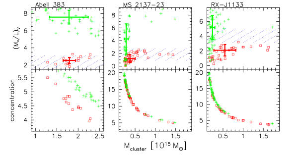
For the dissipational and dissipationless models, the fixed input parameters for the models are the BCG luminosity, half-light radius, and Sersic index ($n=4$). The free parameters are the total cluster mass, $M_{\mathrm{cluster}}$, the dark halo concentration, $c$, and $M_{*}/L$. By randomly selecting these input parameters from a reasonable range, we can find both dissipational and dissipationless models that are within $1$ and $2\sigma$ of the measured central velocity dispersion and radial and tangential arc locations. Projections of these points in $M_{\mathrm{cluster}}$–$c$ space and $M_{\mathrm{cluster}}$–$M_{*}/L$ space are shown in Figure 4. The cluster Abell 383 does not have any models which lie within $1\sigma$ of the observations, so the $2\sigma$ models are plotted instead. These projections show that the best-fit models lie on a tight relation between $M_{\mathrm{cluster}}$ and $c$. From equation 16, halos in this mass range should have a concentration between 3.2 and 5.0, eliminating most of the best-fit models for MS 2137-23 and RXJ-1133. In the case of MS 2137-23, this eliminates almost all of the dissipationless models (squares). However, weak lensing measurements of MS-2137-23 predict a concentration about twice as large as simulations, thereby only eliminating a few models (Gavazzi et al. 2003).

Also illustrated in Figure 4 is the difference in $M_{*}/L$ between the two models. The heavy lines indicate the median and $25-75^{\mathrm{th}}$ percentile (SIQR) for the best-fits for each toy model. As with the comparison to the $L$–$\sigma$ relation, the dissipational models have lower $M_{*}/L$ values than the dissipationless models. For example, the median $(M_{*}/L)_{V}$ ratios for MS 2137-23 are $4.3\pm 2.4$ and $1.2\pm 0.6$ for the dissipationless and dissipational models, respectively. For RX-J1133, $(M_{*}/L)_{B}=2.1\pm 0.8$ for the dissipational models and $(M_{*}/L)_{B}=5.2\pm 1.7$ for the dissipationless models. The best-fit dissipational models all have an $M_{*}/L$ below 2.5(3.5) in the $V(B)$-band. Assuming passive evolution, the expected value of $M_{*}/L$ is $(M_{*}/L)_{B}\approx 4.1\pm 0.95$ at $z\sim 0.35$ (Treu & Koopmans 2004; van der Wel et al. 2004; Treu et al. 2006). The purely dissipational model for RX-J1133 is therefore marginally inconsistent with expected $M_{*}/L$ values. The shaded regions in Figure 4 show the expected ranges for the stellar mass-to-light ratios for the three clusters; MS 2137-23 is consistent with both the dissipational and dissipationless models. Neither the dissipational nor the dissipationless models represent an adequate fit to Abell 383; however, the $M_{*}/L$ values for the dissipational models within $2\sigma$ of the observations are in better agreement with the expected $M_{*}/L$ value.

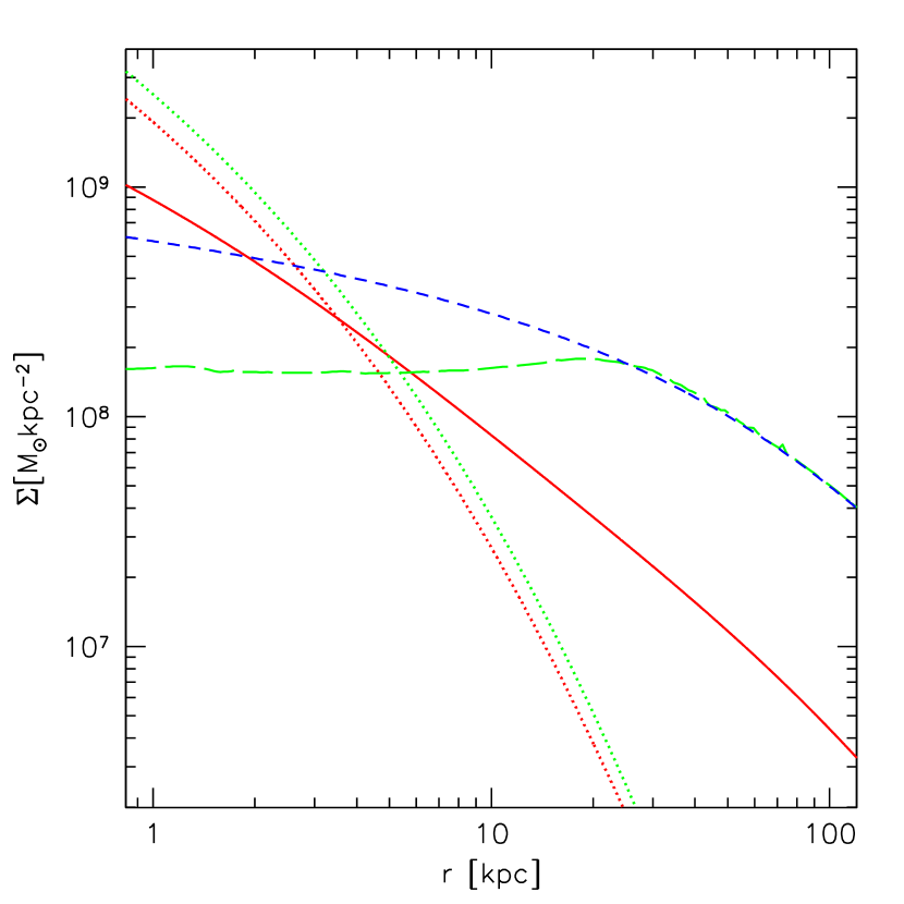
Taking MS 2137-23 as a specific example, Figure 5 plots the stellar and dark matter density of the two models. Both models selected have tangential and radial arcs and velocity dispersions within the error bars of the observations. The best-fit model parameters and the observed model parameters are given in Table 1. For the dissipational model, the dark matter density dominates over the stellar density at all radii. From Sand et al. (2004), the best-fit inner slope of the dark matter profile is 0.57. This is shown along with the $2\sigma$ error bars. The inner slope derived by Sand et al. (2004) depends on the concentration remaining fixed at 400 kpc. If the concentration is allowed to vary, the best-fit inner slope will generally increase by 0.15, bringing it closer to the dissipationless model. However, the dissipationless model also depends strongly on concentration and there exist choices for $M_{\mathrm{cluster}}$, $M_{*}/L$, and $c$, which fit the observations equally well, such that the dissipationless model almost matches an NFW profile.

Table 1Input model parameters for strong lensing BCG and cluster: MS 2137-23

Parameter	Dissipational	Dissipationless
Free (fitted) model parameters
$\log M_{\mathrm{cluster}}/M_{\odot}$	14.75	14.55
concentration ($c$)	8.99	13.27
$(M_{*}/L)_{V}$	1.67	5.47
Observed model parameters
$\log(L_{\mathrm{BCG}}{}/L_{\odot}{})_{V}$	$11.5$	$11.5$
$n_{\mathrm{Sersic}}$	4.0	4.0
${R_{\mathrm{e}}}\ [\mathrm{kpc}]$	$23.03$	$23.03$
$\sigma_{0}\ [\mathrm{km\ s}^{-1}]$	317.33	321.90

Figure 5.— The dark matter and stellar density profiles for two best-fit models to the lensing observations of MS 2137-23. The solid curve is the dark matter and the lower dotted curve is the stellar component of the dissipational model. The dashed curve and the upper dotted curve are the dark matter and stars, respectively, of the dissipationless model. The dash-dotted curve with the shaded region is the best-fit model for the dark matter from Sand et al. (2004) along with $2\sigma$ error bars.

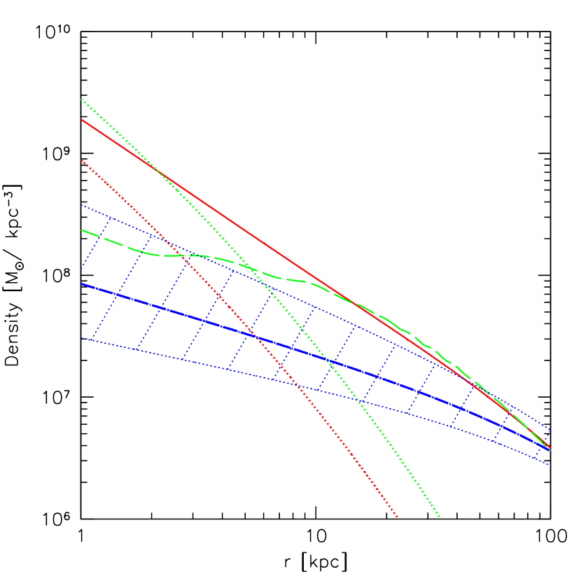
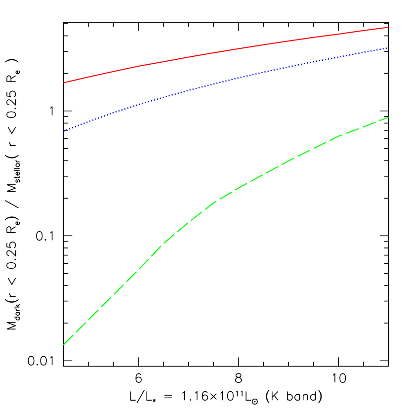
As illustrated by the strong lensing, the differences between the two models for BCGs are small. This is due to the fact that the ratio between the stellar mass of the galaxy and the dark matter halo mass is very small, on the order of $0.002$. Figure 6 shows the ratio of the dark matter to stellar mass inside $0.25{R_{\mathrm{e}}}$ as a function of galaxy luminosity using the scaling relations from §3.1. As the luminosity and cluster mass increase, the differences between the two models and the initial NFW profile become smaller. Therefore, the differences between the dissipational and dissipationless methods of galaxy formation will be most pronounced in smaller dark matter halos, such as fossil groups and isolated ellipticals. In these cases the stellar component of the central galaxy is much larger relative to the halo component, making the differences between the dissipational and dissipationless models more pronounced.

Figure 6.— The ratio of dark to stellar matter contained within $0.25\,{R_{\mathrm{e}}}$ as a function of BCG luminosity. The solid line shows the dissipational model, the dashed line shows the dissipationless model. The dotted line in the center shows the ratio of an NFW profile for the dark matter to a Sersic profile for the stars.

4. Comparison to SAURON Data

Figure 6 illustrates that the total mass-to-light ratio is an increasing function of galaxy luminosity. This is in agreement with the trend found by the SAURON project (Cappellari et al. 2006), which uses integrated-field spectroscopic observations of 25 E/S0 galaxies. Using these observations and stellar population models to determine the stellar mass-to-light ratios for their sample of galaxies, Cappellari et al. (2006) find that the total(dynamical) $M/L$ is consistently larger than $M_{*}/L$ and that this difference increases with increasing stellar mass. This trend is shown in Figure 7. The ‘$\times$’-symbols denote the SAURON data and the shaded region is the best fit. The stellar mass-to-light ratio ($I$-band) is never larger than 3.4 for the brightest galaxies. The best fitting line is given by (Cappellari et al. 2006)

$$\left(M/L\right)_{I}=(2.35\pm 0.19)\left(\frac{L_{I}}{10^{10}L_{\odot}}\right)^{0.32\pm 0.06}\,.$$ (27)

This fit ignores the galaxy (M32) at $M_{I}\sim-17.5$.

Figure 7.— The trend in $M/L$ with galaxy luminoisty observed in the SAURON data (Cappellari et al. 2006). The $M_{*}/L$ values for these galaxies are all below 3.4. The ‘$\times$’-symbols denote the SAURON data. The dotted line and surrounding shaded region show the best fit to the SAURON data. The triangles (squares) show the $M/L$ calculated for the dissipational (dissipationless) models for each SAURON galaxy. The solid and dashed lines show the best fit for the dissipational and dissipationless models, respectively.

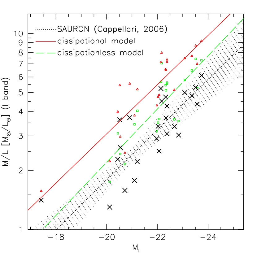
We can compare our dissipational and dissipationless models to the SAURON data to determine whether the models recover the trend given by equation 27. As in the previous section, we assume that each of the 25 galaxies in the Cappellari et al. (2006) study is formed either by purely dissipational or purely dissipationless processes. We fix the stellar mass-to-light ratio, the total $I$-band luminosity, and the effective radius (${R_{\mathrm{e}}}$) for each galaxy to the values given in Cappellari et al. (2006). We then vary the dark matter halo mass for the dissipational and dissipationless models of each galaxy until the velocity dispersion within ${R_{\mathrm{e}}}$ for both models matches the value reported in Cappellari et al. (2006). Since dissipational formation increases the dark matter content in the center of a galaxy compared to the dissipationless model, a smaller total halo mass is required to recover the same central velocity dispersion in the dissipationally formed galaxies than in the dissipationlessly formed galaxies. The differences in halo mass lead to differences in dynamical $M/L$, which are shown in Figure 7. Both the dissipational and dissipationless models reproduce the same trend in $M/L$ with luminosity as is shown in the SAURON data. However, the dissipationless models yield slightly lower $M/L$ values than the dissipational models, leading to better agreement with the observed values. The standard deviation of the SAURON points around the best fit line is 0.11. The standard deviation of the dissipationless model points (squares) around the best-fit line to the SAURON data (dotted line) is 0.14. The same value for the dissipational models is 0.25. However, both the dissipational and dissipationless models have $M/L$ values higher than those from the SAURON data. Therefore, no combination of these models will yield the measured SAURON galaxies. However, both the dissipational and dissipationless models used here assume the stellar orbits are isotropic and that the galaxies are spherically symmetric. Both of these assumptions will affect the model-calculated $M/L$ values; in the case of rotating galaxies, the calculated $M/L$ values will be lowered and possibly brought into better agreement with the SAURON observations.

5. Example Galaxy: NGC 4494

NGC 4494 is an ordinary elliptical galaxy with a $B$-band luminosity of $2.37\times 10^{10}\ L_{\odot}$. Because it is an isolated galaxy instead of a BCG, the mass ratio between the dark matter halo and the stars is smaller and, therefore, the difference between the dissipationless and dissipational models of formation will be larger than those found for BCGs in massive clusters. As with the BCGs, the input model parameters for NGC 4494 can be constrained by observations.

5.1. Velocity Dispersion using Planetary Nebulae

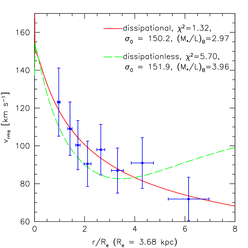
Planetary nebulae have been established as a good mass tracer in the outer regions of galaxies. These observations provide a good comparison case for our extreme models of galaxy formation. Napolitano et al. (2009) measure positions and velocities of planetary nebulae out to $\sim 7\ {R_{\mathrm{e}}}$ in the elliptical NGC 4494, probing the velocity dispersion for the galaxy much farther out than the central velocity dispersion. At these large radii, the dark matter will be comparable to, and dominate over, the stellar matter (see Figure 9), thus emphasizing the differences between the dissipational and dissipationless models. By fixing the luminosity ($L_{B}=2.37\times 10^{10}\ L_{\odot}$), the effective radius (${R_{\mathrm{e}}}=3.68\ \mathrm{kpc}$), and the Sersic index ($n=3.30$), of the model galaxies to observations from Napolitano et al. (2009), we can fit our dissipational and dissipationless models to the planetary nebulae velocity dispersion curves by varying the total halo mass and the stellar mass-to-light ratios. These fits also include a point for the central velocity dispersion, $\sigma=150.2\pm 3.7\ \mathrm{km\ s}^{-1}$, as reported in the Hyperleda database (Paturel et al. 2003). The results are shown in Figure 8. For the dissipational model, $(M_{*}/L)_{B}=2.97$, while the dissipationless model has a mass-to-light ratio of $3.96$. The total halo masses are $6.0\times 10^{11}\ M_{\odot}$ for the dissipational model and $1.0\times 10^{13}\ M_{\odot}$ for the dissipationless model. The slightly poorer quality fit for the dissipationless model is due to the fact that the galaxy’s effective radius is close to the minimum allowed for the galaxy to form via dissipationless mergers ($\sim 2.7\ \mathrm{kpc}$), as discussed above in §2.4. As the galaxy approaches this minimum size, there is insufficient binding energy in some of the central dark matter layers to allow the stellar layers to cross. The fit of the dissipationless model could be improved if we relaxed our model requirement that all the energy from the stars is deposited locally, instead allowing more energy to be deposited in the outer regions of the halo. This could be the case if the orbits of the in-falling material were radial orbits instead of perfectly circular orbits as assumed in this work.

Although the dissipational model shown in Figure 8 provides a better fit to the data, the $B$-band mass-to-light ratio required for the dissipational model is significantly lower than the value derived from stellar population models, $4.3\pm 0.7$ (Napolitano et al. 2009). Thus, a purely dissipational formation of NGC 4494 appears to be ruled out at the $\sim 1.9\sigma$ level.

Figure 8.— The velocity dispersion of NGC 4494 from Napolitano et al. (2009) measured using planetary nebulae. The two lines show the dissipational and dissipationless galaxy formation models. The central velocity dispersion of NGC 4494 is taken to be $150.2\pm 3.7\ \mathrm{km\ s}^{-1}$ (Paturel et al. 2003).

Although adjusting the stellar mass-to-light ratio eliminates the differences in the velocity dispersion profile for these two models, the difference in dark matter density between them remains large (see Figure 9). The inner dark matter density profile for the dissipationless model follows $\sim r^{-0.2}$, while that of the dissipational model follows $\sim r^{-1.7}$, making the central dark matter densities in the two models very different. The slope index of the dark matter in the dissipational model is in good agreement with that predicted for a final isothermal mass distribution in §1.

5.2. Dark Matter Annihilation

Although only available in the Milky Way, one direct method of probing WIMP dark matter currently being explored is the observation of gamma rays from the self-annihilation of WIMP dark matter particles (Stoehr et al. 2003; Colafrancesco et al. 2006; Diemand et al. 2007). The signal strength from such annihilations will be proportional to $\rho_{\mathrm{dark}}^{2}$. Assuming a smooth distribution of dark matter, the ratio of the annihilation signal strength within an aperture of ${R_{\mathrm{e}}}$ for the dissipational and dissipationless models of NGC 4494 is around $1890$, similar to what would be expected for a Milky Way sized halo. Although not observable today, the Fermi gamma-ray space telescope hopes to measure the dark matter annihilation signal from our own galaxy. The large difference in signal strength between the dissipational and the dissipationless models calculated here dominates over the boost in signal strength expected from unresolved substructure, which is of order $10$ (Strigari et al. 2007; Kuhlen et al. 2008), providing another possible test of the formation history of the stellar component of galaxies.

Figure 9.— The projected dark matter density profile for the best-fit models to NGC 4494. The solid line is for the dissipationless model. The long-dashed line is the dissipationless model. The short-dashed line is the best fit NFW. The two dotted lines are the stellar profiles for the dissipationless (upper) and dissipational (lower) models.

6. Conclusions

We have shown that the two extreme cases for the assembly of the stellar content of galaxies lead to large differences in the dark matter density profiles of galaxies, assuming that the initial halo conditions are well-described by N-body simulations. The stellar mass density dominates over the dark matter density in the central regions of both models; the dark matter density in the dissipational models can be as much as two orders of magnitude lower at $r\approx 1\,\mathrm{kpc}$ than the dark matter density in the dissipational models. However, because galaxies are undoubtedly built up by both dissipational and dissipationless accretion, most observations will not easily distinguish between these two models. For example, although the best-fit models for BCGs have different stellar mass-to-light ratios, neither is outside the acceptable range of values from stellar population models and observations. Strong gravitational lensing observations of BCGs and their host clusters show that the dissipational formation models have $M_{*}/L$ values that are marginally too low compared to those expected for passively evolving ellipticals. For RX-J1133, the median $(M_{*}/L)_{B}=2.1\pm 0.8$ and $5.2\pm 1.7$ for the dissipational and dissipationless models, respectively, while the expected $(M_{*}/L)_{B}$ from passive evolution is $4.1\pm 1.0$ (Treu & Koopmans 2004). This discrepancy between $M_{*}/L$ values marginally rules out a purely dissipational formation history for BCGs, in agreement with both theoretical expectations and other observational evidence. Observations of strong lensing by BCGs have been used to effectively rule out dark matter density profiles as steep and steeper than an NFW (Sand et al. 2004), further strengthening arguments against a purely dissipational formation for the stellar component of BCGs. Although extreme values for the concentration ($\sim 10$) and $(M_{*}/L)_{B}$ ($\sim 1.0$) are allowed by the lensing and dynamics data, the dissipational model can be ruled out for a more constrained and plausible set of model parameters.

Both models adequately reproduce the trend of increasing total $M/L$ with galaxy luminosity for E/S0 galaxies, observed using integrated-field spectroscopy by the SAURON project (Cappellari et al. 2006). However, the lower $M/L$ values found for the dissipationless models are in better agreement with the data.

Constraints on the stellar mass-to-light ratios can also be used to exclude the purely dissipational model of galaxy formation in the case of the isolated elliptical, NGC 4494. Fitting the dissipational and dissipationless models to observations of planetary nebulae yields $(M_{*}/L)_{B}$ values of $2.97$ and $3.96$ for the dissipational and dissipationless models, respectively. Compared to $4.3\pm 0.7$, the $(M_{*}/L)_{B}$ inferred from stellar synthesis models, the purely dissipational model can be ruled out at the $1.9\sigma$ level.

Since the change in the dark matter density for both models is directly related to the change in the central mass of the halo, the larger the stellar component is relative to the dark matter halo, the larger the differences between the dissipational and dissipationless extremes will be. Therefore, instead of examining the properties of BCGs, we propose looking for the differences between dissipational and dissipationless formation mechanisms using the brightest galaxies of fossil groups and isolated elliptical galaxies. The large differences attainable in this mass range of galaxies is clearly illustrated by the study of NGC 4494. The dark matter density profiles shown in Figure 9 have inner slope indices of $\alpha\approx 0.2$ and $1.7$ for the dissipationless and dissipational models, respectively. The differences in the dark matter density profiles for galaxies in this mass range are significant enough that they could be probed by galaxy-galaxy weak lensing studies, provided the difference in dark matter slopes is not removed by averaging over many galaxies with different formation histories. Finally, the difference in dark matter content between the dissipational and dissipationless models yields differences in the signal strength from dark matter annihilation of order $\sim 1890$, far larger than the boost factor expected from the unresolved dark matter substructure in the Milky Way halo.

The focus of this paper has been the energetics of the dissipational and dissipationless galaxy formation mechanisms, not the mechanisms themselves. For dissipational galaxy formation, we have assumed that baryons cool and condense in the center of halos, leading to adiabatic contraction of the surrounding dark matter. This behavior has been confirmed in cosmological simulations. Although simplified, the model presented here is correct, on average, for more complicated galaxy formation scenarios, including major as well as minor mergers, and accretion from filaments instead of spherical shells (Gnedin et al. 2004).

The physical mechanism we propose for dissipationless galaxy formation is the dynamical friction of small stellar clumps against a smooth dark matter background. In the models used here, we assume circular orbits for the incoming stellar material. The inclusion of radial orbits and non-spherical galaxies is left for future work, as it requires modeling a combination of dissipational and dissipationless formation mechanisms. We assume that the build-up of the galaxy occurs via a series of small, minor mergers (Bezanson et al. 2009; Cook et al. 2009; Naab et al. 2009), not allowing for equal-mass mergers, which more violently disrupt the system. Indeed, it has been shown in dissipationless N-body simulations that equal-mass merger remnants will retain the profile of the steepest progenitor (Boylan-Kolchin & Ma 2004; Dehnen 2005; Kazantzidis et al. 2006; Vass et al. 2009). Therefore, cuspy dark matter profiles are robust under major mergers. However, if baryons are added to dark matter halos, they will presumably condense more than the dark matter, making up the bulk of the central, high-density matter in merging halos. As two halos merge, the outer, less tightly bound and dark-matter-dominated components will be tidally stripped, but the central high density, predominantly stellar components will settle into the center of the merger remnant, undergoing dynamical friction along the way. Therefore, the baryons are an important ingredient to dry merger scenarios because they ensure the merging clump is sufficiently tightly bound to reach the central regions of the nascent galaxy.

The extreme differences in the inner dark matter halo densities for the dissipational and dissipationless models emphasize the importance of the addition of baryons to dark matter halos. Without introducing modifications to the $\Lambda\mathrm{CDM}$ paradigm, dark matter halo cusps can be reduced to cores via the dissipationless formation of the central stellar regions of galaxies. The balance between dissipational and dissipationless formation mechanisms can be probed by observations. Current observations of BCGs and ellipticals galaxies are sufficient to exclude a purely dissipational formation mechanism for these galaxies. Future measurements of stellar mass-to-light ratios from microlensing observations, and direct detection of dark matter in the Milky Way will help to constrain the balance between dissipational and dissipationless formation mechanisms and the dependence of this balance on time and environment.

References

- Abadi et al. (2009) Abadi, M. G., Navarro, J. F., Fardal, M., Babul, A., & Steinmetz, M. 2009, ArXiv e-prints
- Abadi et al. (2003) Abadi, M. G., Navarro, J. F., Steinmetz, M., & Eke, V. R. 2003, ApJ, 591, 499
- Aubert & Pichon (2007) Aubert, D. & Pichon, C. 2007, MNRAS, 374, 877
- Bernardi et al. (2007) Bernardi, M., Hyde, J. B., Sheth, R. K., Miller, C. J., & Nichol, R. C. 2007, AJ, 133, 1741
- Bernardi et al. (2003) Bernardi, M., Sheth, R. K., Annis, J., Burles, S., Eisenstein, D. J., Finkbeiner, D. P., Hogg, D. W., Lupton, R. H., Schlegel, D. J., SubbaRao, M., Bahcall, N. A., Blakeslee, J. P., Brinkmann, J., Castander, F. J., Connolly, A. J., Csabai, I., Doi, M., Fukugita, M., Frieman, J., Heckman, T., Hennessy, G. S., Ivezić, Ž., Knapp, G. R., Lamb, D. Q., McKay, T., Munn, J. A., Nichol, R., Okamura, S., Schneider, D. P., Thakar, A. R., & York, D. G. 2003, AJ, 125, 1817
- Bezanson et al. (2009) Bezanson, R., van Dokkum, P. G., Tal, T., Marchesini, D., Kriek, M., Franx, M., & Coppi, P. 2009, ApJ, 697, 1290
- Binney & Evans (2001) Binney, J. J. & Evans, N. W. 2001, MNRAS, 327, L27
- Blumenthal et al. (1986) Blumenthal, G. R., Faber, S. M., Flores, R., & Primack, J. R. 1986, ApJ, 301, 27
- Bode et al. (2001) Bode, P., Ostriker, J. P., & Turok, N. 2001, ApJ, 556, 93
- Bode et al. (2009) Bode, P., Ostriker, J. P., & Vikhlinin, A. 2009, ApJ, 700, 989
- Boylan-Kolchin & Ma (2004) Boylan-Kolchin, M. & Ma, C. 2004, MNRAS, 349, 1117
- Cappellari et al. (2006) Cappellari, M., Bacon, R., Bureau, M., Damen, M. C., Davies, R. L., de Zeeuw, P. T., Emsellem, E., Falcón-Barroso, J., Krajnović, D., Kuntschner, H., McDermid, R. M., Peletier, R. F., Sarzi, M., van den Bosch, R. C. E., & van de Ven, G. 2006, MNRAS, 366, 1126
- Cappellari et al. (2009) Cappellari, M., di Serego Alighieri, S., Cimatti, A., Daddi, E., Renzini, A., Kurk, J. D., Cassata, P., Dickinson, M., Franceschini, A., Mignoli, M., Pozzetti, L., Rodighiero, G., Rosati, P., & Zamorani, G. 2009, ApJ, 704, L34
- Colafrancesco et al. (2006) Colafrancesco, S., Profumo, S., & Ullio, P. 2006, A&A, 455, 21
- Cole et al. (2001) Cole, S., Norberg, P., Baugh, C. M., Frenk, C. S., Bland-Hawthorn, J., Bridges, T., Cannon, R., Colless, M., Collins, C., Couch, W., Cross, N., Dalton, G., De Propris, R., Driver, S. P., Efstathiou, G., Ellis, R. S., Glazebrook, K., Jackson, C., Lahav, O., Lewis, I., Lumsden, S., Maddox, S., Madgwick, D., Peacock, J. A., Peterson, B. A., Sutherland, W., & Taylor, K. 2001, MNRAS, 326, 255
- Cook et al. (2009) Cook, M., Lapi, A., & Granato, G. L. 2009, MNRAS, 397, 534
- Cooray & Milosavljević (2005) Cooray, A. & Milosavljević, M. 2005, ApJ, 627, L85
- de Blok et al. (2008) de Blok, W. J. G., Walter, F., Brinks, E., Trachternach, C., Oh, S.-H., & Kennicutt, R. C. 2008, AJ, 136, 2648
- Dehnen (2005) Dehnen, W. 2005, MNRAS, 360, 892
- Desroches et al. (2007) Desroches, L., Quataert, E., Ma, C., & West, A. A. 2007, MNRAS, 377, 402
- Diemand et al. (2007) Diemand, J., Kuhlen, M., & Madau, P. 2007, ApJ, 657, 262
- Diemand et al. (2005) Diemand, J., Zemp, M., Moore, B., Stadel, J., & Carollo, C. M. 2005, MNRAS, 364, 665
- Djorgovski & Davis (1987) Djorgovski, S. & Davis, M. 1987, ApJ, 313, 59
- Dobler et al. (2007) Dobler, G., Keeton, C. R., & Wambsganss, J. 2007, MNRAS, 377, 977
- Dressler et al. (1987) Dressler, A., Lynden-Bell, D., Burstein, D., Davies, R. L., Faber, S. M., Terlevich, R., & Wegner, G. 1987, ApJ, 313, 42
- El-Zant et al. (2001) El-Zant, A., Shlosman, I., & Hoffman, Y. 2001, ApJ, 560, 636
- El-Zant et al. (2004) El-Zant, A. A., Hoffman, Y., Primack, J., Combes, F., & Shlosman, I. 2004, ApJ, 607, L75
- Faber & Jackson (1976) Faber, S. M. & Jackson, R. E. 1976, ApJ, 204, 668
- Flores & Primack (1994) Flores, R. A. & Primack, J. R. 1994, ApJ, 427, L1
- Fukushige & Makino (1997) Fukushige, T. & Makino, J. 1997, ApJ, 477, L9+
- Gao et al. (2004) Gao, L., Loeb, A., Peebles, P. J. E., White, S. D. M., & Jenkins, A. 2004, ApJ, 614, 17
- Gao et al. (2008) Gao, L., Navarro, J. F., Cole, S., Frenk, C. S., White, S. D. M., Springel, V., Jenkins, A., & Neto, A. F. 2008, MNRAS, 387, 536
- Gavazzi et al. (2003) Gavazzi, R., Fort, B., Mellier, Y., Pelló, R., & Dantel-Fort, M. 2003, A&A, 403, 11
- Gentile et al. (2004) Gentile, G., Salucci, P., Klein, U., Vergani, D., & Kalberla, P. 2004, MNRAS, 351, 903
- Gentile et al. (2007) Gentile, G., Tonini, C., & Salucci, P. 2007, A&A, 467, 925
- Georgakakis et al. (2001) Georgakakis, A., Hopkins, A. M., Caulton, A., Wiklind, T., Terlevich, A. I., & Forbes, D. A. 2001, MNRAS, 326, 1431
- Gilmore et al. (2007) Gilmore, G., Wilkinson, M. I., Wyse, R. F. G., Kleyna, J. T., Koch, A., Evans, N. W., & Grebel, E. K. 2007, ApJ, 663, 948
- Gnedin et al. (1999) Gnedin, O. Y., Hernquist, L., & Ostriker, J. P. 1999, ApJ, 514, 109
- Gnedin et al. (2004) Gnedin, O. Y., Kravtsov, A. V., Klypin, A. A., & Nagai, D. 2004, ApJ, 616, 16
- Gonzalez et al. (2005) Gonzalez, A. H., Zabludoff, A. I., & Zaritsky, D. 2005, ApJ, 618, 195
- Graham et al. (1996) Graham, A., Lauer, T. R., Colless, M., & Postman, M. 1996, ApJ, 465, 534
- Graham (2007) Graham, A. W. 2007, MNRAS, 379, 711
- Holley-Bockelmann et al. (2005) Holley-Bockelmann, K., Weinberg, M., & Katz, N. 2005, MNRAS, 363, 991
- Inada et al. (2008) Inada, N., Oguri, M., Becker, R. H., Shin, M.-S., Richards, G. T., Hennawi, J. F., White, R. L., Pindor, B., Strauss, M. A., Kochanek, C. S., Johnston, D. E., Gregg, M. D., Kayo, I., Eisenstein, D., Hall, P. B., Castander, F. J., Clocchiatti, A., Anderson, S. F., Schneider, D. P., York, D. G., Lupton, R., Chiu, K., Kawano, Y., Scranton, R., Frieman, J. A., Keeton, C. R., Morokuma, T., Rix, H.-W., Turner, E. L., Burles, S., Brunner, R. J., Sheldon, E. S., Bahcall, N. A., & Masataka, F. 2008, AJ, 135, 496
- Jardel & Sellwood (2009) Jardel, J. R. & Sellwood, J. A. 2009, ApJ, 691, 1300
- Jesseit et al. (2002) Jesseit, R., Naab, T., & Burkert, A. 2002, ApJ, 571, L89
- Johansson et al. (2009) Johansson, P. H., Naab, T., & Ostriker, J. P. 2009, ApJ, 697, L38
- Kazantzidis et al. (2006) Kazantzidis, S., Zentner, A. R., & Kravtsov, A. V. 2006, ApJ, 641, 647
- Kormendy (1977) Kormendy, J. 1977, ApJ, 218, 333
- Kuhlen et al. (2008) Kuhlen, M., Diemand, J., & Madau, P. 2008, ApJ, 686, 262
- Lauer et al. (2007) Lauer, T. R., Faber, S. M., Richstone, D., Gebhardt, K., Tremaine, S., Postman, M., Dressler, A., Aller, M. C., Filippenko, A. V., Green, R., Ho, L. C., Kormendy, J., Magorrian, J., & Pinkney, J. 2007, ApJ, 662, 808
- Lima Neto et al. (1999) Lima Neto, G. B., Gerbal, D., & Márquez, I. 1999, MNRAS, 309, 481
- Lin & Mohr (2004) Lin, Y.-T. & Mohr, J. J. 2004, ApJ, 617, 879
- Lin et al. (2003) Lin, Y.-T., Mohr, J. J., & Stanford, S. A. 2003, ApJ, 591, 749
- Loeb & Peebles (2003) Loeb, A. & Peebles, P. J. E. 2003, ApJ, 589, 29
- Ma & Boylan-Kolchin (2004) Ma, C. & Boylan-Kolchin, M. 2004, Physical Review Letters, 93, 021301
- McMillan & Dehnen (2005) McMillan, P. J. & Dehnen, W. 2005, MNRAS, 363, 1205
- Milosavljević & Merritt (2001) Milosavljević, M. & Merritt, D. 2001, ApJ, 563, 34
- Moore et al. (1999) Moore, B., Quinn, T., Governato, F., Stadel, J., & Lake, G. 1999, MNRAS, 310, 1147
- Naab et al. (2009) Naab, T., Johansson, P. H., & Ostriker, J. P. 2009, ApJ, 699, L178
- Naab et al. (2007) Naab, T., Johansson, P. H., Ostriker, J. P., & Efstathiou, G. 2007, ApJ, 658, 710
- Napolitano et al. (2009) Napolitano, N. R., Romanowsky, A. J., Coccato, L., Capaccioli, M., Douglas, N. G., Noordermeer, E., Gerhard, O., Arnaboldi, M., de Lorenzi, F., Kuijken, K., Merrifield, M. R., O’Sullivan, E., Cortesi, A., Das, P., & Freeman, K. C. 2009, MNRAS, 393, 329
- Navarro & Benz (1991) Navarro, J. F. & Benz, W. 1991, ApJ, 380, 320
- Navarro et al. (1997) Navarro, J. F., Frenk, C. S., & White, S. D. M. 1997, ApJ, 490, 493
- Navarro & White (1994) Navarro, J. F. & White, S. D. M. 1994, MNRAS, 267, 401
- Neto et al. (2007) Neto, A. F., Gao, L., Bett, P., Cole, S., Navarro, J. F., Frenk, C. S., White, S. D. M., Springel, V., & Jenkins, A. 2007, MNRAS, 381, 1450
- Nipoti et al. (2004) Nipoti, C., Treu, T., Ciotti, L., & Stiavelli, M. 2004, MNRAS, 355, 1119
- Oh et al. (2008) Oh, S.-H., de Blok, W. J. G., Walter, F., Brinks, E., & Kennicutt, R. C. 2008, AJ, 136, 2761
- Ostriker & Hausman (1977) Ostriker, J. P. & Hausman, M. A. 1977, ApJ, 217, L125
- Paczynski (1986) Paczynski, B. 1986, ApJ, 301, 503
- Pahre et al. (1998) Pahre, M. A., de Carvalho, R. R., & Djorgovski, S. G. 1998, AJ, 116, 1606
- Paturel et al. (2003) Paturel, G., Petit, C., Prugniel, P., Theureau, G., Rousseau, J., Brouty, M., Dubois, P., & Cambrésy, L. 2003, A&A, 412, 45
- Peirani et al. (2008) Peirani, S., Kay, S., & Silk, J. 2008, A&A, 479, 123
- Pichon & Aubert (2006) Pichon, C. & Aubert, D. 2006, MNRAS, 368, 1657
- Pooley et al. (2009) Pooley, D., Rappaport, S., Blackburne, J., Schechter, P. L., Schwab, J., & Wambsganss, J. 2009, ApJ, 697, 1892
- Postman & Lauer (1995) Postman, M. & Lauer, T. R. 1995, ApJ, 440, 28
- Rhee et al. (2004) Rhee, G., Valenzuela, O., Klypin, A., Holtzman, J., & Moorthy, B. 2004, ApJ, 617, 1059
- Ricotti (2003) Ricotti, M. 2003, MNRAS, 344, 1237
- Romano-Díaz et al. (2009) Romano-Díaz, E., Shlosman, I., Heller, C., & Hoffman, Y. 2009, ArXiv e-prints
- Romano-Díaz et al. (2008) Romano-Díaz, E., Shlosman, I., Hoffman, Y., & Heller, C. 2008, ApJ, 685, L105
- Romanowsky et al. (2003) Romanowsky, A. J., Douglas, N. G., Arnaboldi, M., Kuijken, K., Merrifield, M. R., Napolitano, N. R., Capaccioli, M., & Freeman, K. C. 2003, Science, 301, 1696
- Sand et al. (2004) Sand, D. J., Treu, T., Smith, G. P., & Ellis, R. S. 2004, ApJ, 604, 88
- Schechter & Wambsganss (2002) Schechter, P. L. & Wambsganss, J. 2002, ApJ, 580, 685
- Sersic (1968) Sersic, J. L. 1968, Atlas de galaxias australes (Cordoba, Argentina: Observatorio Astronomico, 1968)
- Simon et al. (2005) Simon, J. D., Bolatto, A. D., Leroy, A., Blitz, L., & Gates, E. L. 2005, ApJ, 621, 757
- Spekkens et al. (2005) Spekkens, K., Giovanelli, R., & Haynes, M. P. 2005, AJ, 129, 2119
- Spergel & Steinhardt (2000) Spergel, D. N. & Steinhardt, P. J. 2000, Physical Review Letters, 84, 3760
- Springel et al. (2008) Springel, V., Wang, J., Vogelsberger, M., Ludlow, A., Jenkins, A., Helmi, A., Navarro, J. F., Frenk, C. S., & White, S. D. M. 2008, MNRAS, 391, 1685
- Stoehr et al. (2003) Stoehr, F., White, S. D. M., Springel, V., Tormen, G., & Yoshida, N. 2003, MNRAS, 345, 1313
- Strigari et al. (2007) Strigari, L. E., Koushiappas, S. M., Bullock, J. S., & Kaplinghat, M. 2007, Phys. Rev. D, 75, 083526
- Subramanian et al. (2000) Subramanian, K., Cen, R., & Ostriker, J. P. 2000, ApJ, 538, 528
- Swaters et al. (2003) Swaters, R. A., Madore, B. F., van den Bosch, F. C., & Balcells, M. 2003, ApJ, 583, 732
- Tonini et al. (2006) Tonini, C., Lapi, A., & Salucci, P. 2006, ApJ, 649, 591
- Tremaine & Weinberg (1984) Tremaine, S. & Weinberg, M. D. 1984, MNRAS, 209, 729
- Treu et al. (2006) Treu, T., Koopmans, L. V., Bolton, A. S., Burles, S., & Moustakas, L. A. 2006, ApJ, 640, 662
- Treu & Koopmans (2004) Treu, T. & Koopmans, L. V. E. 2004, ApJ, 611, 739
- Vale & Ostriker (2008) Vale, A. & Ostriker, J. P. 2008, MNRAS, 383, 355
- Valenzuela et al. (2007) Valenzuela, O., Rhee, G., Klypin, A., Governato, F., Stinson, G., Quinn, T., & Wadsley, J. 2007, ApJ, 657, 773
- van der Wel et al. (2004) van der Wel, A., Franx, M., van Dokkum, P. G., & Rix, H.-W. 2004, ApJ, 601, L5
- van Dokkum et al. (2008) van Dokkum, P. G., Franx, M., Kriek, M., Holden, B., Illingworth, G. D., Magee, D., Bouwens, R., Marchesini, D., Quadri, R., Rudnick, G., Taylor, E. N., & Toft, S. 2008, ApJ, 677, L5
- Vass et al. (2009) Vass, I. M., Kazantzidis, S., Valluri, M., & Kravtsov, A. V. 2009, ApJ, 698, 1813
- Wambsganss (2006) Wambsganss, J. 2006, Gravitational Microlensing (Gravitational Lensing: Strong, Weak and Micro, Saas-Fee Advanced Courses, Volume 33. ISBN 978-3-540-30309-1. Springer-Verlag Berlin Heidelberg, 2006, p. 453), 453–+
- Weinberg (1986) Weinberg, M. D. 1986, ApJ, 300, 93
- Weinberg & Katz (2002) Weinberg, M. D. & Katz, N. 2002, ApJ, 580, 627
- Wetzel & White (2009) Wetzel, A. R. & White, M. 2009, ArXiv e-prints
- Woźniak et al. (2000) Woźniak, P. R., Udalski, A., Szymański, M., Kubiak, M., Pietrzyński, G., Soszyński, I., & Żebruń, K. 2000, ApJ, 540, L65