Exit times in non-Markovian drifting continuous-time random walk processes

Abstract

By appealing to renewal theory we determine the equations that the mean exit time of a continuous-time random walk with drift satisfies both when the present coincides with a jump instant or when it does not. Particular attention is paid to the corrections ensuing from the non-Markovian nature of the process. We show that when drift and jumps have the same sign the relevant integral equations can be solved in closed form. The case when holding times have the classical Erlang distribution is considered in detail.

I Introduction

In this article we study exit times of continuous-time random walks (CTRWs) with drift. By this we understand a random process $X_{t}$ whose evolution in time can be thought of as the result of the combined effect of a constant drift and the occurrence of random jumps. Thus, for $t\geqslant t_{0}$ we define

$$X_{t}=X_{t_{0}}+v(t-t_{0})+S_{t},\quad S_{t}=\sum_{n=1}^{\infty}J_{n}\ \theta(t-t_{n}),$$ (1)

where $\theta(u)=1$ for $u\geqslant 0$, $t_{n}=\tau_{1}+\cdots+\tau_{n}$ are the jump times, $J_{n}$ the jump magnitude and $v>0$ by convention. Note that as the notation suggests, $t_{0}$ coincides with a jump. The process $X_{t}$ may represent physically the position of a diffusing particle, for instance. All through this paper we will assume that (i) the sojourn times $\tau_{n}>0$ are independent and identically distributed (i.i.d.) random variables with probability density and cumulative distribution function (PDF and, respectively, CDF) $\psi(t)$ and $\Psi(t)=\int_{0}^{t}\psi(t^{\prime})dt^{\prime}$; (ii) $\{J_{n}\}$ is a sequence of i.i.d. random variables with common PDF $h(\cdot)$; and (iii), that $J_{m}$ is independent of $\tau_{n}$ for any $n,m$.

In absence of drift, and when the holding times $\tau_{n}$ are exponentially distributed, $\tau_{n}\sim\mathcal{E}(\lambda)$ for some $\lambda>0$, the jump process $S_{t}$ is a classical compound Poisson process (CPP) characterized by having independent increments $S_{t+h}-S_{t}$; in addition the associated “arrival-process” $N_{t}\equiv\sum_{n=1}^{\infty}\theta(t-t_{n})$ is Poisson distributed: $N_{t}\sim\mathcal{P}(\lambda t)$. Therefore, drift-less CTRWs can be considered as a generalization of CPPs where the holding times of the processes $S_{t}$ are arbitrarily distributed. In statistical physics such drift-less CTRWs have been widely used after the work of Montroll $\&$ Weiss mw65 ; w94 and their relevant statistical properties, like correlation functions and the behavior in the continuum limit,  a subject of intense interest JT74 ; JT76 ; Go ; Sch . Applications of CTRWs can be found in the study of transport in disordered media (e.g., Sch ; ms84 ; Weiss-porra ; Margolin1 ), anomalous relaxation in polymer chains Hu , sandpile and earthquake modeling (e.g., hs02 ; Me03 ), random networks Be , self-organized criticality in granular systems Bo , scaling properties of Lévy walks Ku , electron tunneling Gu , transmission tomography OW ; OW2 , distribution of matter in the universe Os71 and changes in stock markets due to unexpected catastrophes m76 . More recently, the use of CTRWs has been advocated to give a microscopic, tick-by-tick, description of financial markets: see mmw03 ; mmp05 ; mmpw06 ; mpmlmm05 ; s09 . A comprehensive review of CTRW applications in finance and economics is given in s06 .

Physically, the introduction of these general CTRWs stems from the fact that in many settings the exponential holding-time assumption may be inadequate to describe the physical situation —see Me03 ; mmw03 . Additional motivation arises from the observation that there is an extensive number of different physical systems that show some sort of anomalous diffusion —a subject of great interest from the viewpoint of statistical physics in the last years—, and that this anomalous behavior can well described by fractional Fokker-Planck equations obtained after imposing the continuum limit on CTRW models Metzler ; s07 ; m07 .

The further addition of the drift term to a CTRW, as we do in Eq. (1), is a natural and significant incorporation. The resulting process —which can be viewed as the discrete analogue of a (fractional) diffusion with drift— is known for playing a fundamental role in the modeling of the cash flow at an insurance company j03 ; zyl10 and, more recently, it has been shown that it also rules the rate of energy dissipation in nonlinear optical fibers VM1 . Indeed, present and forthcoming results can be also of interest in transport in amorphous media Ba , models of decision and response time in psychology Sm and neuron dynamics Sm2 .

In all these scenarios one is faced with the basic problem of determining the first-passage time for a CTRW with drift, a question that has been theoretically considered in the past m87 ; m92 ; c97 ; cmc97 ; rd00a ; rd00b ; MB ; is07 . The usual approach taken there entails the computation of transition and first-passage time distributions of the process, e.g. m92 ; MB , and the results are typically obtained under the assumption of the continuum limit rd00a ; rd00b ; MB ; is07 . This procedure has incontestable advantages for obtaining the leading-order behavior, but it is not adequate for a detailed analysis of the statistical properties of the process at the inter-jump timescale, as in mmw03 ; mpmlmm05 ; j03 ; zyl10 ; VM1 .

Motivated by the above, here we pose the problem of evaluating the mean exit time from the interval $(0,b)$ of a drifting CTRW $X_{t}$ when the only available information is the present state $X_{r}=x$, where $r\geqslant 0$ is the present chronological time —note that, by adjusting the time clock and spatial scale, the results carry over to any interval $(a,b)$ and initial time $t_{0}$. Here $X_{t}$ is given by Eq. (1) where $S_{t}$ is the jump part and $N_{t}$ the associated counting process (a renewal process). In the drift-less case previous work in this regard includes that of mmp05 ; mmpw06 where a linear integral equation for the mean escape time after a jump off a given interval is derived. We note however that these results do not cover a generic situation. Indeed, while for CPPs (as for the general Lévy processes) Markov property implies that results derived starting at a jump time carry over to arbitrary present, no such inference is possible for a generic CTRW due to its non-Markovian nature. Thus, escape times depend on the actual state and available information and hence the question as to how to generalize the former results to general present time $r$ appears naturally. We remark that implications ensuing from the lack of Markovianess have been ignored at large in the literature, a gap that we have intended to fill in —see VM2 . In particular, it remains an open question to what extent dropping the assumption that “the present is a jump time” affects the relevant probabilities. Here we address these issues and generalize the results of mmp05 ; mmpw06 in a twofold way by assuming that (i) a drift $vt>0$ operates on the system and (ii) the present $r$ is an arbitrary time, not necessarily a jump instant, and the observer has knowledge of the present, but not of the history, of the system.

The interest of this problem goes far beyond the purely academic since such a situation may appear in several different physical contexts. For example, one might be interested in predicting the mean time for an insurance/financial company to go bankrupt from the knowledge of just the actual company budget, i.e., when the information regarding the company’s past performance has not been disclosed. A second example is provided by the study of the distribution of inhomogeneities in an optical fiber; it was found VM1 that the signal’s energy amplitude at a point $t$ ($t$ is the spatial variable in this setting) involves a CTRW with drift $X_{t}$; in this context  one typically knows only the value of the energy at the observation point $r$, not on the whole fiber. More generally the approach will be relevant in situations where either the elapsed time between events is “large” (it might be as large as years, in a context of catastrophes observation) or when the event’s times $t_{n}$ are not physically measurable observables and only mean escape times are. (Note that both the mean exit time and initial time are typically macroscopic magnitudes.)

The article is structured as follows. In Section II we show how the solution to these problems involves ideas drawn from renewal theory and solve the simpler case when $v=0$. The case $v>0$ is considered in the next sections where it is found that key properties of the obtained equation depend on the sign of the jumps. In Section III it is shown that if this sign is positive the solution can be given in closed form by Laplace transformation —cf. Eqs. (12) and (13). For the case when drift and jumps have opposite signs we find integral equations that the relevant objects satisfy, see Section IV, but no closed solution can be given in a general situation. Section V addresses the most general scenario in which jumps $J_{n}$ can take both signs. Solvable cases are discussed there.

In all cases we exemplify our results by considering the particular instance when sojourn times have Erlang distribution, $\mathcal{E}r(\lambda,2)$. $\mathcal{E}r(\lambda,n)$ corresponds to having a sum of $n$ independent exponential variables and hence generalizes the exponential density in a natural way,

$$\psi(t)=\frac{\lambda^{n}t^{n-1}}{(n-1)!}e^{-\lambda t},\,n\in\mathbb{N},\,t\geqslant 0,$$ (2)

while it maintains an adequate capability to fit measured data. From a physical perspective these facts make this density a natural candidate to describe multi-component systems which operate only when several independent, exponentially distributed operations have been completed or whenever there is a hidden Poissonian flux of information and jumps only appear as the outcome of two or more consecutive arrivals. This explains the interest that it has drawn in the field of information traffic sb00 ; fc02 . Similarly the appearance of this distribution to model transaction orders in financial markets can also be expected since it takes, at least, two arrivals (buy and sell orders) for a transaction to be completed. For further applications to ruin problems and insurance see dh01 ; lg04 .

II The problem

Recall that we aim to study exit times of a drifting CTRW $X_{t}$ given the present state $X_{r}=x$. To this end let $r+\mathbf{t}_{b}^{x,r}$ be the first time past $r$ at which $X_{t}$ exits $(0,b)$; $T_{b}(x,r)$ be its expected value: $T_{b}(x,r)=\mathbb{E}[\mathbf{t}_{b}^{x,r}]$; finally let $\mathbb{T}_{b}(x)$ denote the mean exit time off $(0,b)$ after a jump $t_{n}$ (loosely one has $\mathbb{T}_{b}(x)=T_{b}(x,t_{n}),n=0,\dots,\infty$; however the relation between both quantities is not trivial, as we see below in Section III). Note also that here and elsewhere we use $\mathbb{E}[\cdot]$ to denote expectation.

In the exponential Markov case $\mathbf{t}_{b}^{x,r}$ is independent of $r$, $T_{b}(x,r)=\mathbb{T}_{b}(x)$ and it only remains to formulate (and solve) the equation that this object satisfies. However this situation no longer holds in the generic, non-Markovian case where $\mathbf{t}_{b}^{x,r}$ does depend on $r$. We find (see below and Section III) that the relation between $T_{b}(x,r)$ and $\mathbb{T}_{b}(x)$ involves the “excess life” $E_{r}\equiv t_{N_{r}+1}-r$, or time elapsed until the next arrival occurs. We now sketch classical renewal theory (see kt81 ; c65 and Go ) that shows how to construct the CDF $\Phi(t|r)\equiv\mathbb{P}\{E_{r}\leqslant t\}$ of $E_{r}$.

Let $m(t)\equiv\mathbb{E}[N_{t}]$ be the mean number of jumps up to $t$: the renewal function. It satisfies the integral renewal equation

$$m(t)=\Psi(t)+\int_{0}^{t}m(t-t^{\prime})\psi(t^{\prime})dt^{\prime}.$$ (3)

Then, by using the total probability theorem it can be proved that

$$\Phi(t|r)=\int^{r+t}_{r}\left[1-\Psi(r+t-t^{\prime})\right]dm(t^{\prime}).$$ (4)

Upon solution of the above integral equations we obtain $\Phi(t|r)$. Actually, they can be solved with all generality by recourse to Laplace transformation. Let $\hat{g}(s)$ be the Laplace transform of a function $g(t)$ so that

$$g(t)=\frac{1}{2\pi i}\int_{c-i\infty}^{c+i\infty}e^{st}\hat{g}(s)ds,\ c>0.$$ (5)

Then, Eqs. (3) and (4) allow to recover the distribution of $E_{r}$ in closed form via

$$\hat{m}(s) = \frac{1}{s}\frac{\hat{\psi}(s)}{1-\hat{\psi}(s)},$$ (6a)

$$\hat{\phi}(s|r) = e^{sr}\left[1-\hat{\psi}(s)\right]\int_{r}^{\infty}e^{-sl}\hat{m}(l)ldl,$$ (6b)

where $\hat{m}(s)$ and $\hat{\phi}(s|r)$ are the Laplace transforms of $m(t)$ and $\phi(t|r)\equiv\partial_{t}\Phi(t|r)$.

If $v=0$ these expressions can be used to relate $T_{b}(x,r)$ and $\mathbb{T}_{b}(x)$. Indeed let $t_{N_{r}}\equiv t_{n}$, say, be the “last” jump time and $E_{r}^{-}\equiv r-t_{n}$ the time elapsed from $t_{n}$ to the present. Then, with $E_{r}^{+}\equiv E_{r}$ one obviously has that $E_{r}^{-}+E_{r}^{+}=t_{n+1}-t_{n}\equiv\tau_{n+1}$, and that the exit time right after $t_{n}$ is that after $r$, $\mathbf{t}_{b}^{x,r}$, plus $E_{r}^{-}$, and hence

$$\mathbb{T}_{b}(x)=\mathbb{E}[E_{r}^{-}]+\mathbb{E}[\mathbf{t}_{b}^{x,r}]=\mathbb{E}[\tau_{n+1}]-\mathbb{E}[E_{r}^{+}]+T_{b}(x,r).$$ (7)

Thus, $T_{b}(x,r)$ follows adding a correction term to $\mathbb{T}_{b}(x)$ which depends only on $r$. Finally $\mathbb{T}_{b}(x)$ is obtained by solving a linear integral equation —see mmp05 ; mmpw06 . Unfortunately when $v\neq 0$ this simple argument fails as then knowledge of the present position does not entail its knowledge at $t_{n}$. In the next sections we derive the relevant correction to the mean exit time. This correction depends now in all parameters $r$, $x$ and $b$ —see Eqs. (9) and (26) below.

III Jump process with favorable drift

In this section we consider the case when both drift and jumps have a positive sign, i.e. when $X_{t}$ is increasing. As a result, the process can only leave the interval through the upper boundary $b$. Let us assume that at time $t=r$ the system is in $X_{r}=x\in(0,b)$, and that the excess life $E_{r}$ is known in advance, $E_{r}=l$. If the excess life is longer than $\varrho\equiv{b-x\over v}<l$, the drift will drive the process out of the region at time $r+\varrho$, before the next jump takes place at $t_{N_{r}+1}$. Conversely, if $l\leqslant\varrho$ at least a jump of size $J_{N_{r}+1}=u$ will occur prior to exiting the interval. Note that just before $t_{N_{r}+1}$ the process $X_{t}$ is no longer at $x$, but at $x+vl$. Therefore, two possible scenarios appear: either the jump size is larger than the remaining distance up to the upper boundary, $u\geqslant b-x-vl$, and the process leaves the interval at $r+E_{r}$, or it does not. In the latter case the problem renews from $t=r+l$, $X_{r+l}=x+vl+u$, so the mean escape time will be increased by an amount $\mathbb{T}_{b}\left(x+vl+u\right)$. It can be proven that these considerations imply that $T_{b}(x,r)$ must satisfy —recall that $\psi(\cdot)$, $h(\cdot)$ are the waiting-time and, respectively, jump PDFs— the following equation

$$T_{b}(x,r)=\left[1-\Phi\left(\varrho|r\right)\right]\varrho+\int^{\varrho}_{0}l\phi(l|r)\int^{\infty}_{b-x-vl}h(u)dudl$$

$$+\int^{\varrho}_{0}\phi(l|r)\int^{b-x-vl}_{0}h(u)\left[l+\mathbb{T}_{b}\left(x+vl+u\right)\right]dudl,$$ (8)

an expression that relates $T_{b}(x,r)$ and $\mathbb{T}_{b}(x)$. Note that since $\Phi\left(l|r\right)$ depends on $r$ so it does the mean time $T_{b}(x,r)$. Finally, after some rearrangement, Eq. (8) can be conveniently written as

$$T_{b}(x,r)=\int^{\varrho}_{0}\left[1-\Phi\left(l|r\right)\right]dl$$

$$+\frac{1}{v}\int^{v\varrho}_{0}\phi\left(\left.\varrho-\frac{z}{v}\right|r\right)\int^{z}_{0}h(u)\mathbb{T}_{b}\left(b-z+u\right)dudz.$$ (9)

Similarly, by letting $r\to 0$, we find that $\mathbb{T}_{b}(x)$ must satisfy

$$\mathbb{T}_{b}(x)=\int^{\varrho}_{0}\left[1-\Psi(l)\right]dl$$

$$+\frac{1}{v}\int^{v\varrho}_{0}\psi\left(\varrho-\frac{z}{v}\right)\int^{z}_{0}h(u)\mathbb{T}_{b}\left(b-z+u\right)dudz,$$ (10)

$x\in(0,b)$. Equation (9) along with (10) allow us to solve the posed problem. The second of these defines an integral equation for $\mathbb{T}_{b}(x)$ which, if $v=0$, reduces upon appropriate change to that of mmp05 ; mmpw06 . It is remarkable that Eq. (10) can be solved in a fully explicit way. To this end we define the allied object $\mathbb{F}(y)$, as the solution of the following integral equation

$$\mathbb{F}(y)=\int^{y/v}_{0}\left[1-\Psi(l)\right]dl$$

$$+\frac{1}{v}\int^{y}_{0}\psi\left(\frac{y-z}{v}\right)\int^{z}_{0}h(u)\mathbb{F}\left(z-u\right)dudz,$$ (11)

for $y\in\mathbb{R}^{+}$. Then it follows that $\mathbb{T}_{b}(x)=\mathbb{F}(b-x)$, for $x\in(0,b)$. We note further that taking a Laplace transformation in Eq. (11) we find that

$$\hat{\mathbb{F}}(s)=\frac{1}{vs^{2}}\frac{1-\hat{\psi}(sv)}{1-\hat{\psi}(sv)\hat{h}(s)},$$ (12)

where $\hat{\mathbb{F}}(s)\equiv\int^{\infty}_{0}\mathbb{F}(y)e^{-sy}dy$, $\hat{h}(s)\equiv\int^{\infty}_{0}h(u)e^{-su}du$, and $\hat{\psi}(s)\equiv\int^{\infty}_{0}\psi(s)e^{-st}dt$. Here $s=s_{R}+is_{I}$ is complex and $s_{R}\geqslant 0$. Further, we also have

$$\hat{J}(s|r)=\hat{\mathbb{F}}(s)-\frac{1-\hat{h}(s)}{vs^{2}\left[1-\hat{\psi}(sv)\hat{h}(s)\right]}\left[\hat{\phi}(sv|r)-\hat{\psi}(sv)\right],$$ (13)

where the correction to the mean time after a jump is clearly displayed and again, for convenience, we defined $J(y|r)\equiv T_{b}(b-y|r)$, and extended (9) to $y\geqslant 0$. Thus ${\mathbb{F}}(y)$ and $J(y|r)$ can be recovered by Laplace inversion, cf. Eq. (5), and $\mathbb{T}_{b}(x)$ and $T_{b}(x|r)$ will eventually follow.

Equation (13) has several mathematical limits of applied interest. We first consider the situation when $v$ is small. Let $\mu\equiv\leavevmode\nobreak\ \mathbb{E}[\tau_{n+1}]$, $\mu_{r}\equiv\leavevmode\nobreak\ \mathbb{E}[E_{r}]$; then, using that $\hat{\psi}(sv)=1-\mu sv+O(v^{2})$ and so forth we see that for small $v$, $\hat{J}(s|r)$ has an expansion in powers of $v$ as

$$\hat{J}(s|r)=\hat{\mathbb{F}}(s)-\frac{\mu-\mu_{r}}{s}-\frac{\hat{h}(s)}{1-\hat{h}(s)}(\mu-\mu_{r})\mu v+O(v^{2}),$$ (14)

which implies, in particular, Eq. (7). Another interesting case is obtained letting $r\to\infty$: the steady-state solution. This limit is relevant since it can be associated to a situation in which the only information available to the observer is the present value of the stochastic process, not even the starting point. Recalling that by the renewal theorem $\underset{t\to\infty}{\lim}m(t)/t=1/\mu$, Eqs. (6) and (13) yield

$$\hat{\phi}(s|\infty) = \frac{1-\hat{\psi}(s)}{s\mu},$$ (15)

$$\hat{J}(s|\infty) = \hat{\mathbb{F}}(s)-\frac{1-\hat{h}(s)}{v^{2}s^{3}\mu}\frac{1-(1+sv\mu)\hat{\psi}(sv)}{1-\hat{\psi}(sv)\hat{h}(s)}.$$ (16)

We illustrate the ideas above by detailing the case when jump magnitudes have an exponential distribution $h(u)=\gamma e^{-\gamma u}$, where $\gamma>0$ is a real parameter, and sojourn times an Erlang distribution $\tau_{n}\sim\mathcal{E}r(\lambda,2)$. Hence

$$\hat{h}(s)=\frac{\gamma}{\gamma+s},\quad\hat{\psi}(s)=\frac{\lambda^{2}}{(\lambda+s)^{2}}.$$ (17)

In this case Eq. (11) yields that $\hat{\mathbb{F}}(s)$ is the following rational function

$$\hat{\mathbb{F}}(s)=\frac{1}{vs^{2}}\frac{2\lambda\gamma v+v(2\lambda+\gamma v)s+v^{2}s^{2}}{\lambda(\lambda+2\gamma v)+v(2\lambda+\gamma v)s+v^{2}s^{2}}.$$ (18)

Hence, the mean escape time of $(0,b)$ after a jump is

$$\mathbb{T}_{b}(x)=\frac{2\gamma v}{\lambda+2\gamma v}\varrho$$

$$+\frac{\lambda^{2}}{z_{+}-z_{-}}\left[\frac{1-e^{-z_{-}\varrho}}{z_{-}^{2}}-\frac{1-e^{-z_{+}\varrho}}{z_{+}^{2}}\right],$$ (19)

where we recall that $v\varrho=b-x$ is the initial distance to the boundary $b$ and

$$z_{\pm}\equiv\lambda+\frac{\gamma v}{2}\left(1\pm\sqrt{1-\frac{4\lambda}{\gamma v}}\right),$$ (20)

with $\mbox{Re}[z_{\pm}]>0$.

The evaluation of the mean exit time starting at $r$, $T_{b}(x,r)$, involves the renewal function and excess-life distribution. We first obtain from Eq. (6)

$$\hat{m}(s)=\frac{\lambda^{2}}{s^{2}(2\lambda+s)},\quad\hat{\phi}(s|r)=\hat{\psi}(s)+\frac{(1-e^{-2\lambda r})s\lambda}{2(\lambda+s)^{2}}.$$ (21)

By inversion we get $m(t)=\big{(}2\lambda t+e^{-2\lambda t}-1\big{)}/4$ and

$$\ \Phi(t|r)=1-e^{-\lambda t}\left[1+\left(\frac{1+{e^{-2\lambda r}}}{2}\right)\lambda t\right].$$ (22)

Then by using Eq. (13) we find at last that

$$T_{b}(x,r)=\mathbb{T}_{b}(x)$$

$$-\frac{\lambda}{2}\frac{1-e^{-2\lambda r}}{z_{+}-z_{-}}\left[\frac{1-e^{-z_{-}\varrho}}{z_{-}}-\frac{1-e^{-z_{+}\varrho}}{z_{+}}\right].$$ (23)

Plots of this function in terms of $x$ are given in Fig. 1 for several values of $r$ and a certain choice of the rest of parameters.

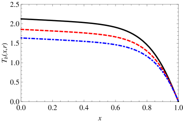
Figure 1: (Color online) Sample representations of $T_{b}(x,r)$ for different values of $r$: $r=0$, i.e. $\mathbb{T}_{b}(x)$, solid (black) line, $r=0.4$, dashed (red) line and $r=10.0$, dot-dashed (blue) line. The rest of the parameters were chosen as follows: $b=1.0$, $v=0.1$, $\lambda=1.0$ and $\gamma=0.1$.

Finally note how, in particular, if $v=0$ then

$$\mathbb{T}_{b}(x)=\frac{2}{\lambda}\left[1+\gamma(b-x)\right] = \mathbb{E}[\tau_{n}]\left(1+\frac{b-x}{\mathbb{E}[J_{n}]}\right),$$ (24)

$$T_{b}(x,r) = \mathbb{T}_{b}(x)-\frac{1-e^{-2\lambda r}}{2\lambda}.$$ (25)

IV The case of opposite drift and jumps

We now consider the case when the sign of the drift $vt>0$ is opposite to that of the jumps. In this case the process can leave the interval through both the upper and the lower boundaries: the drift pushes steadily the process up, whereas the jumps threaten the system with a downside exit. The resulting process is a prototype model in risk management to describe the dynamics of the cahsflow $X_{t}$ at an insurance company under the assumption that premiums are received at a constant rate $v>0$ and that the company incurs in losses $J_{n}<0$ from claims reported at times $t_{n},n=1,\dots\infty$ (the Cramer-Lundberg model).

As before, we analyze the evolution starting at $t=r$ with $X_{r}=x$. Then if $E_{r}=l$, $l>\varrho$, the drift will drive the process out of the region through the upper boundary at time $r+\varrho$. Otherwise ($l\leqslant\varrho$) at least a jump $J_{N_{r}+1}=-u$, say, occurs at time $t_{N_{r}+1}$ before escape, and two possible scenarios appear depending on the relative magnitudes of the jump size and the location of the process right before the jump, $X_{t}=x+vl$: for $u\geqslant x+vl$ the process will leave the interval through the lower boundary at $r+E_{r}$, but when $u<x+vl$ the process after the jump will remain inside the interval, $X_{r+l}=x+vl-u$, the exit problem will start afresh, and the mean escape time will be increased by $\mathbb{T}_{b}\left(x+vl-u\right)$. Again these considerations imply that $T_{b}(x,r)$ and $\mathbb{T}_{b}(x)$ must satisfy for $0<x<b$

$$T_{b}(x,r)=\left[1-\Phi\left(\varrho|r\right)\right]\varrho+\int^{\varrho}_{0}l\phi(l|r)\int^{\infty}_{x+vl}h(u)dudl$$

$$+\int^{\varrho}_{0}\phi(l|r)\int^{x+vl}_{0}h(u)\left[l+\mathbb{T}_{b}\left(x+vl-u\right)\right]dudl$$

$$=\int^{\varrho}_{0}\left[1-\Phi\left(l|r\right)\right]dl$$

$$+\frac{1}{v}\int^{b}_{x}\phi\left(\left.\frac{z-x}{v}\right|r\right)\int^{z}_{0}h(u)\mathbb{T}_{b}\left(z-u\right)dudz,$$

(26)

$$\mathbb{T}_{b}(x)=\int^{\varrho}_{0}\left[1-\Psi(l)\right]dl$$

$$+\frac{1}{v}\int^{b}_{x}\psi\left(\frac{z-x}{v}\right)\int^{z}_{0}h(u)\mathbb{T}_{b}\left(z-u\right)dudz.$$

(27)

Hence $T_{b}(x,r)$ follows in terms of quadratures also in this case, given $\mathbb{T}_{b}(x)$. Unfortunately, unlike what happens for the case considered in the previous Section, Eq. (27) can not be solved in closed form for arbitrary PDFs $\psi(\cdot)$ and $h(\cdot)$. Further progress can be made for Erlang times, $\mathcal{E}r(\lambda,2)$. Indeed, in this case (27) reads

$$\mathbb{T}_{b}(x)=\frac{2-\left(2+\lambda\varrho\right)e^{-\lambda\varrho}}{\lambda}$$

$$+\frac{\lambda^{2}}{v^{2}}\int^{b}_{x}\left(z-x\right)e^{-\lambda\left(z-x\right)/v}\int^{z}_{0}h(u)\mathbb{T}_{b}\left(z-u\right)dudz,$$ (28)

and hence, by differentiation we find that $\mathbb{T}_{b}(x)$, for $0<x<b$, also satisfies the following integral-differential equation:

$$\mathbb{T}_{b}^{\prime\prime}(x)-\frac{2\lambda}{v}\mathbb{T}_{b}^{\prime}(x)+\frac{\lambda^{2}}{v^{2}}\mathbb{T}_{b}(x)=\frac{2\lambda}{v^{2}}$$

$$+\frac{\lambda^{2}}{v^{2}}\int^{x}_{0}h(u)\mathbb{T}_{b}\left(x-u\right)du,$$ (29)

subject to the following boundary conditions:

$$\lim_{x\to b}\mathbb{T}_{b}(x)=0,\mbox{ and }\lim_{x\to b}\mathbb{T}_{b}^{\prime}(x)=-1/v.$$ (30)

We first consider a general solution to this equation extending it to the full real axis, so we will drop the subscript in $\mathbb{T}_{b}(x)$. We find a solution by Laplace transformation as

$$\hat{\mathbb{T}}(s)=\frac{2\lambda/s+(Bv-2\lambda A)v+Av^{2}s}{\lambda^{2}[1-\hat{h}(s)]-2\lambda vs+v^{2}s^{2}},$$ (31)

where $A$ and $B$ are $\mathbb{T}(0)$ and $\mathbb{T}^{\prime}(0)$ respectively. By inversion, cf. Eq. (5), $\mathbb{T}(x)$ follows in terms of $A$ and $B$. By requiring (30) we obtain a linear algebraic system for $A$ and $B$, which upon solution yields $\mathbb{T}_{b}(x)$ in closed form.

To be specific we consider the case when jumps are also exponentially distributed: $h(x)=\gamma e^{-\gamma x}$. Then we have (17) and $\hat{\mathbb{T}}(s)$ is the rational function

$$\hat{\mathbb{T}}(s)=\frac{(\gamma+s)[2\lambda+(Bv-2\lambda A)vs+Av^{2}s^{2}]}{s^{2}[\lambda(\lambda-2\gamma v)+(\gamma v-2\lambda)vs+v^{2}s^{2}]}.$$ (32)

Upon re-scale of constants the inverse Laplace transform of (32) reads

$$\left(\frac{\lambda}{2}-\gamma v\right)\mathbb{T}(x)$$

$$=\tilde{A}+\gamma x+\left[\frac{\lambda}{v^{2}}(\lambda-\lambda\tilde{A}+v\tilde{B})-\frac{\tilde{B}}{2}\xi_{-}\right]\frac{e^{\xi_{+}x}-1}{\xi_{+}(\xi_{+}-\xi_{-})}$$

$$-\left[\frac{\lambda}{v^{2}}(\lambda-\lambda\tilde{A}+v\tilde{B})-\frac{\tilde{B}}{2}\xi_{+}\right]\frac{e^{\xi_{-}x}-1}{\xi_{-}(\xi_{+}-\xi_{-})},$$

with

$$\xi_{\pm}\equiv\frac{\lambda}{v}-\frac{\gamma}{2}\pm\frac{\gamma}{2}\sqrt{1+\frac{4\lambda}{\gamma v}}.$$ (34)

Unfortunately the final expressions for $\tilde{A}$ and $\tilde{B}$ after imposing (30) are not very illuminating so we do not transcribe them here. Sampling values for different parameter specifications can be found in Fig. 2.

The limit $b\to\infty$ is interesting as $\mathbb{T}_{\infty}(x)$ gives the probability that $X_{t}$ ever hits $0$. This corresponds to the classical ruin probability in an insurance context. It turns out that $\mathbb{T}_{\infty}(x)$ can be determined in a direct way that avoids solving the aforementioned linear system. Without proof  we note that if $\lambda>2\gamma v$ then

$$\mathbb{T}_{\infty}(x)=\frac{2(1+\gamma x)}{\lambda-2\gamma v}=\left(1+\gamma x\right)\Big{/}\left(\frac{1}{\mathbb{E}[\tau_{n}]}-\frac{v}{\mathbb{E}[J_{n}]}\right),$$ (35)

while $\mathbb{T}_{\infty}(x)=\infty$ otherwise. Once $\mathbb{T}_{b}(x)$ is known, $T_{b}(x,t)$ follows again by integration —see Fig. 2.

(a)
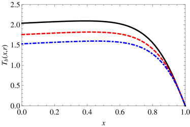
(b)

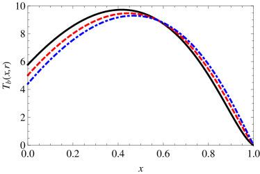
Figure 2: (Color online) Sample representations of $T_{b}(x,r)$ for different values of $r$: $r=0$, i.e. $\mathbb{T}_{b}(x)$, solid (black) line, $r=0.4$, dashed (red) line and $r=10.0$, dot-dashed (blue) line. The rest of the parameters were chosen as follows, $b=1.0$, $v=0.1$, $\lambda=1.0$ and (a) $\gamma=0.1$; (b) $\gamma=4.0$. We see how, when drift and jumps have a different sign, an interesting behavior may appear in $T_{b}(x,r)$. In the upper panel we observe that this function is no longer decreasing with $x$ and has a maximum in the interior of the interval, cf. Fig. 1. In the lower panel we observe how a cross-over phenomenon may eventually take place reflecting the fact that $\mathbb{T}_{b}(x)$ need not be greater than $T_{b}(x,r)$: this behavior can be traced to the fact that as $r$ increases the jump probability increases, which results in a reduction of the escape time if the process is in the vicinity of the lower boundary but in an increment when close to the upper boundary. The maxima position moves toward greater values of $x$ for larger choices of $r$, in both cases.

V Two-sided jump process with drift

We finally consider the general case corresponding to a jump process where $J_{n}$ can take both signs and hence can exit $(0,b)$ through either of the boundaries. The relevant analysis is similar to that of the last section if one incorporates the possibility of an upper exit due to a jump: If $E_{r}=l>\varrho$ the drift drives directly the process through the upper boundary. If $l\leqslant\varrho$ at least a jump occurs before the exit of the process. When the size $u$ of this jump is positive and $u\geqslant b-x-vl$ the process leaves the interval at time $r+E_{r}$ through the upper boundary, when $u\leqslant-(x+vl)<0$ the exit takes place through the lower boundary, otherwise the process remains inside the interval $(0,b)$ and the problem restarts. Skipping minor details we obtain that $\mathbb{T}_{b}(x)$ and $T_{b}(x,r)$ satisfy respectively

$$T_{b}(x,r)=\int^{\varrho}_{0}\left[1-\Phi\left(l|r\right)\right]dl$$

$$+\frac{1}{v}\int^{b}_{x}\phi\left(\left.\frac{z-x}{v}\right|r\right)\int^{b-z}_{-z}h(u)\mathbb{T}_{b}\left(z+u\right)dudz,$$ (36)

and

$$\mathbb{T}_{b}(x)=\int^{\varrho}_{0}\left[1-\Psi\left(l\right)\right]dl$$

$$+\frac{1}{v}\int^{b}_{x}\psi\left(\frac{z-x}{v}\right)\int^{b-z}_{-z}h(u)\mathbb{T}_{b}\left(z+u\right)dudz.$$ (37)

In a general situation, the latter integral equation is not solvable in closed form. To gain some insight we use the decomposition $h(x)=qh_{+}(x)+ph_{-}(x)$ where $p$ is the probability that a given jump be negative, $q\equiv 1-p$ and $h_{\pm}(\cdot)$ are the jump PDF in the positive/negative regions, i.e. $h_{+}(x)\equiv h(x)\theta(x)\big{/}q$, say.

Note that if $h_{-}(x)=0,\forall x\leqslant 0$, we recover the case considered in Section III, solvable via Laplace transformation. It turns out that we can still construct an analytic closed solution in the more general case when $h_{-}(x)$ vanishes only on $(-b,0)$ —but not on $(-\infty,-b]$. In such a case a negative jump will drive the process out of the interval $(0,b)$ through the lower boundary. Thus $p$ is related to the ruin risk in a economic scenario or to the breakdown probability in a physical system. The equation for $\mathbb{T}_{b}(x)$ reads in this case

$$\mathbb{T}_{b}(x)=\int^{\varrho}_{0}\left[1-\Psi\left(l\right)\right]dl$$

$$+\frac{q}{v}\int^{b}_{x}\psi\left(\frac{z-x}{v}\right)\int^{b-z}_{0}h_{+}(u)\mathbb{T}_{b}\left(z+u\right)dudz,$$ (38)

while a similar expression, with $\phi(\cdot|r)$ in place of $\psi(\cdot)$, holds for $T_{b}(x,r)$. Note that these equations are independent of the form of $h_{-}(\cdot)$ and apart from the factor $q$ in front of the second term they resemble Eqs. (9) and (10); it follows that we can resort to the same technique used in Section III: We consider

$$\mathbb{F}(y)=\int^{y/v}_{0}\left[1-\Psi(l)\right]dl$$

$$+\frac{q}{v}\int^{y}_{0}\psi\left(\frac{y-z}{v}\right)\int^{z}_{0}h(u)\mathbb{F}\left(z-u\right)dudz,$$ (39)

for $y\in\mathbb{R}^{+}$ which is again solvable by means of a Laplace transform; then $\mathbb{T}_{b}(x)$ follows from $\mathbb{T}_{b}(x)=\mathbb{F}(b-x)$ for $x\in(0,b)$. With the previous selection for $h(\cdot)$ and $\psi(\cdot)$, Eq. (17), and in terms of $z=sv$ we find

$$\hat{\mathbb{F}}(s)=\frac{v}{z}\frac{2\lambda\gamma v+(2\lambda+\gamma v)z+z^{2}}{p\lambda^{2}\gamma v+\lambda(\lambda+2\gamma v)z+(2\lambda+\gamma v)z^{2}+z^{3}}.$$ (40)

We first consider the case when $\lambda=\gamma v$. Under this assumption $\hat{\mathbb{F}}(s)$ has poles at $z=z_{j}\equiv\lambda\left(q^{1/3}e^{2\pi ij/3}-1\right)$, $j\in\{1,2,3\}$, and $z=0$. Inverse Laplace transformation yields the mean exit time as

$$\mathbb{T}_{b}(x)=\frac{2}{p\lambda}+\sum_{j=1}^{3}\frac{1+q^{-1/3}e^{-2\pi ij/3}}{3z_{j}}e^{z_{j}\varrho}.$$ (41)

Returning to the general case we see that the inversion of the Laplace transform involves solving a cubic equation, and though explicit formulas are available the resulting expression is awkward. Still, the large $b$ limit can be discerned with all generality. To this end we note that by appealing to Hurwitz’s stability criteria it can be proven that all three roots $z_{j}$, $j\in\{1,2,3\}$, of the denominator in expression (40) —apart from $z=0$— have negative real parts. Hence, evaluating the inversion integral by residues we find

$$\mathbb{T}_{b}(x)=\frac{2}{p\lambda}+\sum_{j=1}^{3}C_{j}e^{z_{j}\varrho},$$ (42)

where $C_{j}$ are certain constants. Thus, letting $b\to\infty$ we see that $\mathbb{T}_{b}(x)\underset{b\to\infty}{\to}\frac{2}{p\lambda}=\frac{\mathbb{E}[\tau_{n}]}{1-\mathbb{E}[\theta(J_{n})]}$.

The evaluation of the correction to $T_{b}(x,r)$ does not present particular difficulties. We leave it as an exercise to the interested reader.

VI Conclusions

We have analyzed the mean exit time for a general CTRW with drift. If the present coincides with a jump time we find that it satisfies a certain integral equation whose solvability is analyzed. We consider next the generic case when the present is an arbitrary instant and the history of the system is not available to the observer and only the present state is. It turns out that the corresponding escape time can be obtained by incorporating an appropriate correction, which can be described in terms of the “excess life”, a familiar object in renewal theory. We find that when the drift and jump components have the same sign the equations that these objects satisfy can be solved in closed form via Laplace transformation, irrespective of the distribution; otherwise, one must restrict to particular choices of the sojourn-time distribution. The case corresponding to the classical Erlang distribution is analyzed in detail. The more general case when jumps take both positive and negative signs is also considered and solved under certain severe conditions. We plan to generalize these ideas to a more general class of waiting-time distributions and pinpoint conditions that guarantee the reducibility of the original formulation to simpler differential equations.

The relevance of these results from a physical perspective is discussed in several connections of interest including possible applications to risk, finance and distribution of energy in optical systems, which will be the matter of future publications. We also point out the relevance of the approach whenever the time between events is “large” or when the arrival times are not physical observables.

Appendix A Some remarks on the continuum limit and its relationship with fractional diffusions

In this appendix we sketch how the approach followed in this article, based in the use of renewal theory, compares with the most traditional one which relies on the previous computation of first-passage time PDFs.

In particular, we shall stress the connections of both techniques under the continuum limit approximation. This concept —which we will define properly in short— can be loosely identified with the limit in which both the mean sojourn time $\mu$ and the characteristic jump magnitude tend to zero —note that, by contrast, in this paper we have considered a situation wherein sojourn times are moderate or even large.

The major benefit of the continuum assumption is that it allows to obtain general results on the basis of limited knowledge of the jumping time and size PDFs, even when these distributions do not have all their moments well defined. The major drawback within our set-up is that as $\mu\to 0$ the variable $r$, the time elapsed from the last known jump, tends to zero as well, and the distinction between $T_{b}(x,r)$ and $\mathbb{T}_{b}(x)$ becomes irrelevant. Therefore, any comparison between the two methods must be focused on how the object $\mathbb{T}_{b}(x)$ is obtained.

Let us assume, for instance, that $\hat{\psi}(s)\sim 1-\mu s+o(s)$ and $\hat{h}(s)\sim 1-k|s|^{\alpha}+o(|s|^{\alpha})$ when $s\to 0$ for certain constants $\mu$, the mean sojourn time, and $k$. (Note however that it is also possible to consider the continuum limit in the case in which the mean sojourn time does not exist. We are just giving an illustrative example. For a more exhaustive analysis of this topic see Metzler .)

To be more explicit, let us consider the case

$$h(u)=\frac{k}{2\sqrt{\pi u^{3}}}e^{-\frac{k^{2}}{4u}}\quad(u>0),$$ (43)

so that,

$$\hat{h}(s)=e^{-k\sqrt{s}}\sim 1-k\sqrt{s}+o(\sqrt{s}).$$ (44)

It is well known that for the CTRW process $S_{t}$, Eq. (1), the propagator $p(u,t)du\equiv\Pr\{u<S_{t}\leqslant u+du\}$ reads in the Laplace-Laplace domain

$$\hat{p}(s_{1},s_{2})=\frac{1}{s_{2}}\frac{1-\hat{\psi}(s_{2})}{1-\hat{\psi}(s_{2})\hat{h}(s_{1})}\sim\frac{\mu}{\mu s_{2}+k\sqrt{s_{1}}},$$ (45)

as $s_{1,2}\to 0$. The continuum limit is recovered in this case by letting $\mu\to 0$, $k\to 0$ with $k/\mu\to K$ finite. The process arising after this limit fulfills the following fractional diffusion equation

$$\partial_{t}p(u,t)+K\ _{0}D_{u}^{\frac{1}{2}}p(u,t)=0,$$ (46)

where ${}_{0}D_{u}^{\frac{1}{2}}$ is the Riemann-Liouville fractional operator of order $\frac{1}{2}$, and whose solution reads

$$p(u,t)=\frac{Kt}{2\sqrt{\pi u^{3}}}e^{-\frac{K^{2}t^{2}}{4u}}.$$ (47)

Let us now define $\Pi_{b}(x,t)$ as the probability that the process $X_{t}$ has never touched $b$ when it started at $x<b$ at the initial time, i.e.

$$\Pi_{b}(x,t)\equiv\Pr\{X_{t^{\prime}}<b,0\leqslant t^{\prime}\leqslant t|X_{0}=x\}.$$ (48)

In the present case, as $S_{t}$ is an increasing positive process and $v>0$, it can be computed by direct integration of $p(u,t)$:

$$\Pi_{b}(x,t)=\int_{0}^{b-x-vt}p(u,t)du=\text{Erfc}\left(\frac{K^{2}t^{2}}{2\sqrt{b-x-vt}}\right).$$ (49)

Now one can obtain $\mathbb{T}_{b}(x)$ through

$$\mathbb{T}_{b}(x)=\int_{0}^{\frac{b-x}{v}}t\partial_{t}\left[1-\Pi_{b}(x,t)\right]dt=\int_{0}^{\frac{b-x}{v}}\Pi_{b}(x,t)dt$$

$$=\frac{4v}{\sqrt{\pi}K^{2}}\int_{0}^{\infty}\left(\xi\sqrt{\xi^{2}+\frac{K^{2}(b-x)}{v^{2}}}-\xi^{2}\right)e^{-\xi^{2}}d\xi$$

$$=\frac{2}{K}\sqrt{\frac{b-x}{\pi}}+\frac{v}{K^{2}}\left[e^{\frac{K^{2}(b-x)}{v^{2}}}\text{Erfc}\left(\frac{K}{v}\sqrt{b-x}\right)-1\right].$$

(50)

Alternatively, if we use the direct approach followed in this paper our results imply that the mean arrival time follows by inversion of the Laplace expression in Eq. (12) when $\mu\to 0$, $k\to 0$ with $k/\mu\to K$ finite

$$\hat{\mathbb{F}}(s)=\frac{1}{vs^{2}}\frac{1-\hat{\psi}(sv)}{1-\hat{\psi}(sv)\hat{h}(s)}\rightarrow\frac{1}{vs^{2}+Ks^{\frac{3}{2}}},$$ (51)

that is

$$\mathbb{T}_{b}(x)=\frac{1}{2\pi i}\int_{c-i\infty}^{c+i\infty}\frac{e^{s(b-x)}}{vs^{2}+Ks^{\frac{3}{2}}}ds.$$ (52)

Upon evaluation of this integral the result (50) is recovered.

References

- (1) E. W. Montroll and G. H. Weiss, J. Math. Phys. 6, 167-181 (1965).
- (2) G. H. Weiss, Aspects and Applications of the Random Walk (North-Holland, Amsterdam, 1994).
- (3) J. K. E. Tunaley, J. Stat. Phys. 11, 397-408 (1974).
- (4) J. K. E. Tunaley, J. Stat. Phys. 14, 461-463 (1976).
- (5) C. Godreche and J. M. Luck, J. Stat. Phys. 104, 489-524 (2001).
- (6) M. F. Shlesinger, J. Stat. Phys. 10, 421-434 (1974).
- (7) E. W. Montroll and M. F. Shlesinger, Nonequilibrium Phenomena II: From stochastics to hydrodynamics. In: J. L. Lebowitz, E. W. Montroll (Eds.), pp. 1-121 (North-Holland, Amsterdam, 1984).
- (8) G. H. Weiss, J. M. Porrà, and J. Masoliver, Phys. Rev. E 58, 6431-6439 (1998).
- (9) G. Margolin and B. Berkowitz, Phys. Rev. E 65, 031101 (2002).
- (10) B. D. Hughes, E. W. Montroll, and M. F. Shlesinger, J. Stat. Phys. 28, 111-126 (1982).
- (11) A. Helmstetter and D. Sornette, Phys. Rev. E 66, 061104 (2002).
- (12) M. S. Mega, P. Allegrini, P. Grigolini, V. Latora, and L. Palatella, Phys. Rev. Lett. 90, 188501 (2003).
- (13) B. Berkowitz and H. Scher, Phys. Rev. Lett. 79, 4038-4041 (1997).
- (14) M. Boguñá and Á. Corral, Phys. Rev. Lett. 78, 4950-4953 (1997).
- (15) R. Kutner, Chem. Phys. 284, 481-505 (2002).
- (16) E. Gudowska-Nowak and K. Weron, Phys. Rev. E 65, 011103 (2002).
- (17) L. Dagdug, G. H. Weiss, and A. H. Gandjbakhche, Phys. Med. Biol. 48, 1361-1370 (2003).
- (18) O. K. Dudko and G. H. Weiss, Diff. Fund. 2, 1-21 (2005).
- (19) V. S. Oskanian and V. Yu. Terebizh, Astrophysics 7, 48-54 (1971).
- (20) R. C. Merton, J. Financ. Econ. 3, 125-144 (1976).
- (21) J. Masoliver, M. Montero, and G. H. Weiss, Phys. Rev. E 67, 021112 (2003).
- (22) J. Masoliver, M. Montero, and J. Perelló, Phys. Rev. E 71, 056130 (2005).
- (23) J. Masoliver, M. Montero, J. Perelló, and G. H. Weiss, J. Econ. Behav. Organ. 61, 577-598 (2006).
- (24) M. Montero, J. Perelló, J. Masoliver, F. Lillo, S. Micciché, and R. N. Mantegna, Phys. Rev. E 72, 056101 (2005).
- (25) G. Germano, M. Politi, E. Scalas, and R. L. Schilling, Phys. Rev.E 79, 066102 (2009).
- (26) E. Scalas, Physica A 362, 225-239 (2006).
- (27) R. Metzler and J. Klafter, Phys. Rep. 339, 1-77 (2000).
- (28) E. Scalas, R. Gorenflo, and F. Mainardi, Phys. Rev. E 69, 011107 (2004).
- (29) F. Mainardi, R. Gorenflo, and A. Vivoli, J. Comput. Appl. Math. 205, 725-735 (2007).
- (30) M. Jacobsen, Stoch. Process Their Appl. 107, 29-51 (2003).
- (31) Z. Zhanga, H. Yanga, and S. Li, J. Comput. Appl. Math. 233, 1773-1784 (2010).
- (32) J. Villarroel and M. Montero, J. Phys. B (to appear, preprint available at arXiv:1003.4408).
- (33) V. Balakrishnan, Physica A 132, 569-580 (1985).
- (34) P. L. Smith, J. Math. Psychol. 44, 408-463 (2000).
- (35) P. L. Smith and T. Van Zandt, Br. J. Math. Stat. Psychol. 53, 293-315 (2000).
- (36) J. Masoliver, Phys. Rev. A 35, 3918-3928 (1987).
- (37) J. Masoliver, Phys. Rev. A 45, 2256-2262 (1992).
- (38) A. Compte, Phys. Rev. E 55, 6821-6831 (1997).
- (39) A. Compte, R. Metzler, and J. Camacho, Phys. Rev. E 56, 1445-1454 (1997).
- (40) G. Rangarajan and M. Ding, Fractals 8, 139-145 (2000).
- (41) G. Rangarajan and M. Ding, Phys. Rev. E. 62, 120-133 (2000).
- (42) G. Margolin and B. Berkowitz, Physica A 334, 46-66 (2004).
- (43) J. Inoue and N. Sazuka, Phys. Rev. E. 76, 021111 (2007).
- (44) J. Villarroel and M. Montero, Chaos Solitons Fractals 42, 128-137 (2009).
- (45) B. H. Soong and J. A. Barria, IEEE Commun. Lett. 4, 402-404 (2000).
- (46) Y. Fang and I. Chlamtac, IEEE Trans. Commun. 50, 396-399 (2002).
- (47) D. C. M. Dickson and C. Hipp, Insur. Math. Econ. 29, 333-334 (2001).
- (48) S. Li and J. Garrido, Insur. Math. Econ. 34, 391-408 (2004).
- (49) D. R. Cox, Renewal Theory (John Wiley and Sons, New York, 1965).
- (50) S. Karlin and H. Taylor, A first course in stochastic processes (Acad. press, New York, 1981).