Magnetic anisotropy of epitaxial (Ga,Mn)As on (113)A GaAs

Abstract

The temperature dependence of magnetic anisotropy in $(113)\mathrm{A}$ (Ga,Mn)As layers grown by molecular beam epitaxy is studied by means of superconducting quantum interference device (SQUID) magnetometry as well as by ferromagnetic resonance (FMR) and magnetooptical effects. Experimental results are described considering cubic and two kinds of uniaxial magnetic anisotropy. The magnitude of cubic and uniaxial anisotropy constants is found to be proportional to the fourth and second power of saturation magnetization, respectively. Similarly to the case of (001) samples, the spin reorientation transition from uniaxial anisotropy with the easy axis along the $[\overline{1}10]$ direction at high temperatures to the biaxial $\langle 100\rangle$ anisotropy at low temperatures is observed around 25 K. The determined values of the anisotropy constants have been confirmed by FMR studies. As evidenced by investigations of the polar magnetooptical Kerr effect, the particular combination of magnetic anisotropies allows the out-of-plane component of magnetization to be reversed by an in-plane magnetic field. Theoretical calculations within the $p-d$ Zener model explain the magnitude of the out-of-plane uniaxial anisotropy constant caused by epitaxial strain but do not explain satisfactorily the cubic anisotropy constant. At the same time the findings point to the presence of an additional uniaxial anisotropy of unknown origin. Similarly to the case of (001) films, this additional anisotropy can be explained by assuming the existence of a shear strain. However, in contrast to the (001) samples, this additional strain has an out of the (001) plane character.

I Introduction

Since many decades, a lot of attention has been devoted to ferromagnetic semiconductors. More recently, the intense research has been triggered by the synthesis of the (III,Mn)V diluted magnetic semiconductor (Ga,Mn)As,Ohno et al. (1996) which has become the canonical example of a dilute ferromagnetic semiconductor.Matsukura et al. (2002); Dietl (2008) It has been demonstrated that a number of pertinent properties of this material can be explained by the $p-d$ Zener model.Dietl et al. (2000, 2001); Jungwirth et al. (2006); Dietl (2008) Magnetic anisotropy of strained (Ga,Mn)As layers can be calculated within this theory, and many experimental studiesTang et al. (2003); Welp et al. (2003); Sawicki et al. (2004, 2005); Wang et al. (2005a); Liu et al. (2006); Thevenard et al. (2007); Gourdon et al. (2007); Gould et al. (2008) were devoted to verify its predictions. However, despite these intense studies, some important features of magnetic anisotropy in this system are at present not completely understood.

An example of such a property is a rather strong in-plane uniaxial magnetic anisotropy of epitaxial (Ga,Mn)As layers grown on GaAs substrates of $(001)$ orientation. Owing to the presence of the twofold symmetry axes $[100]$ and $[010]$, the in-plane zinc-blende directions $[110]$ and $[\overline{1}10]$ are expected to be equivalent. Yet, as implied by the character of magnetic anisotropy, the symmetry is lowered from $D_{2d}$ to $C_{2v}$, possibly due to the growth-induced lack of symmetry between the bottom and the top of the layer,Welp et al. (2004); Sawicki et al. (2004, 2005) which can be phenomenologically described by introducing a shear strain.Sawicki et al. (2005); Zemen et al. (2009); Glunk et al. (2009)

Since these symmetry considerations are limited to $(001)$ layers, investigation of layers grown on substrates of other orientations may not only allow to compare experimental observations with predictions of the $p-d$ Zener model in a more general situation, but also provide information from which conclusions on the nature of the additional anisotropy can be drawn.

In this paper we present results of studies on $\mathrm{Ga}_{1-x}\mathrm{Mn}_{x}\mathrm{As}$ layers grown by low-temperature molecular beam epitaxy (MBE) on GaAs substrates with the $(113)\mathrm{A}$ orientation. Previously, magnetic anisotropy in such films was probed at low temperatures by magnetoresistanceWang et al. (2005b); Limmer et al. (2006a, b), scanning Hall probe microscopyPross et al. (2006) and ferromagnetic resonance measurements.Limmer et al. (2006b); Bihler et al. (2006); Liu and Furdyna (2007) Experimental techniques employed here include superconducting quantum interference device (SQUID) magnetometry, ferromagnetic resonance (FMR), and polar magnetooptical Kerr effect (PMOKE). Our measurements are carried out over a wide temperature and magnetic field range. We find that magnetic anisotropy can be consistently described taking into account three contributions: a uniaxial anisotropy with the hard axis tilted from $[113]$ toward the $[001]$ direction, an in-plane uniaxial anisotropy with the easy axis along the $[\overline{1}10]$ direction, and a cubic anisotropy with easy $\langle 100\rangle$ directions. The general form of anisotropy is, therefore, similar to the case of (001) films, but the direction of the hard axis is found to be neither along [001] nor perpendicular to the film plane in the (113) case. The accumulated experimental results allow us to determine how the three relevant magnetic anisotropy constants $K$ as well as the tilt angle depend on the temperature. We find that the magnitudes of energies corresponding to the competing cubic and uniaxial anisotropies in the (001) plane depend, as could be expected, as the fourth and second power of spontaneous magnetization $M(T)$, respectively. In contrast, a complex dependence on $M(T)$ is observed in the case of the energy characterizing the out-of-plane uniaxial anisotropy. We assign this behavior to the spin-splitting-induced and, hence, temperature dependent redistribution of holes between the valence band subbands that are characterized by different directions of the angular momentum and, hence, of the easy axes.

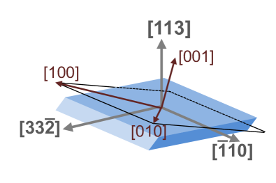
Figure 1: (Color online) Crystallographic directions for a GaAs substrate of (113) orientation.

In the theoretical part, we present a theory of magnetic anisotropy in epitaxially strained layers of (Ga,Mn)As and related systems within the $p-d$ Zener model. Our approach generalizes earlier theories developed for (001) filmsDietl et al. (2000, 2001); Abolfath et al. (2001); Glunk et al. (2009); Zemen et al. (2009) by allowing for an arbitrary crystallographic orientation of the substrate. Similarly to previous studies,Sawicki et al. (2005); Zemen et al. (2009) in order to explain the experimental findings, we introduce an additional shear strain whose three components constitute adjustable parameters. We also take into account the Hamiltonian terms linear in $k$ and find that they give a minor contribution to the magnitude of magnetic anisotropy constants.

II Samples and experiment

We study a 50 nm thick $\mathrm{Ga}_{1-x}\mathrm{Mn}_{x}\mathrm{As}$ layer which has been grown on a (113)A GaAs substrate (see Fig. 1) by low temperature MBE.Reinwald et al. (2005) The total Mn concentration of $x=6.4\%$ has been determined by means of secondary ion mass spectrometry, however only more than twice lower value of an effective Mn concentration $x_{\text{eff}}$ can be inferred from low temperature experimental saturation magnetization, $M_{\text{exp}}$. This reduction of $x$ is primarily caused by a presence of Mn interstitials. These point defects act as double donors and form strongly coupled spin singlet pairs with neighbor substitutional Mn cations.Jungwirth et al. (2006); Yu et al. (2002); Blinowski and Kacman (2003) These pairs neither participate in the ferromagnetic order, nor they contribute to $M$. Thus, the effective concentration of Mn ions which generates $M_{\text{exp}}$ gets reduced to $x_{\text{eff}}=x-2x_{\text{I}}$, where $x_{\text{I}}N_{0}$ is the concentration of the Mn interstitials and $N_{0}$ is the cation concentration. However, the experimentally measured $M_{\text{exp}}$ is further reduced by holes magnetization, $M_{h}$, which is oppositely oriented to magnetization of Mn spins, $M_{\text{Mn}}$, and so $M_{\text{Mn}}$ = $M_{\text{exp}}$ + $|M_{h}|$ should be used to calculate $x_{\text{eff}}$, with $M_{h}$ being computed in the framework of the the mean-field $p-d$ Zener model.Dietl et al. (2000, 2001) We perform these calculations in a self-consistent way taking the hole concentration as $p=N_{0}(x-3x_{\text{I}})=N_{0}(3x_{\text{eff}}-x)/2$, that is neglecting other charge compensating defects.

The open air post growth annealing at temperatures below or comparable to the growth temperatureHayashi et al. (2001); Edmonds et al. (2002) is a frequently used procedure for improving material parameters of (Ga,Mn)As, since the corresponding out-diffusion and passivation of Mn interstitialsEdmonds et al. (2004) increases $x_{\text{eff}}$, $p$, and eventually the Curie temperature $T_{\mathrm{C}}$. Therefore in order to widen the parameter space employed here to study the magnetic anisotropy in this compound we investigate both the as-grown material (sample S1) and the samples annealed at $200^{\circ}$C for 1.5 hour (sample S2) and 5 hours (sample S3). Taking the determined values of $M_{\text{exp}}$ data we end up with $x_{\text{eff}}$ = 2.7, 3.1, and 3.3% and $p=2.0$, 3.3, and $3.8\times 10^{20}$ cm^-3 for which calculated values of $T_{\mathrm{C}}$ = 46, 73, and 85 K compares favorably with the experimentally established values of 65, 77, and 79 K, for samples S1, S2, and S3, respectively.

Magnetic properties referred to above and described further on have been obtained by employing a Quantum Design MPMS XL-5 magnetometer. A special demagnetization procedure has been employed to minimize the influence of parasite fields on zero-field measurements. The temperature dependence of remnant magnetization, TRM, serves to obtain an overview of magnetic anisotropy as well as to determine $T_{\mathrm{C}}$ (Sec. III.1). After cooling the sample across $T_{\mathrm{C}}$ down to $5\,\mathrm{K}$ in the external magnetic field of 0.1 T, the field is removed, allowing magnetization to assume the direction along the closest easy axis. The magnitude of the magnetization component along the magnet axis, TMR_i, is then measured while heating, where $i$ indicates one of the three mutually orthogonal directions of the magnetizing field, corresponding to the surface normal $\bm{n}_{1}=[113]$ and the two edges $\bm{n}_{2}=[33\overline{2}]$, $\bm{n}_{3}=[\overline{1}10]$, as depicted in Fig. 1. Since, except to the immediate vicinity of the spin reorientation transition, magnetization of (Ga,Mn)As films tend to align in a single domain state, the measurements performed for the three orthogonal axes provide the temperature dependence of the magnetization magnitude and direction.

To study magnetic anisotropy in a greater detail, magnetic hysteresis loops $M_{i}(H)$ have been recorded in external magnetic field in the range of $\pm 0.5$ T along the three directions $i$. The measurements have been carried out at various temperatures, and the parameters of the anisotropy model (Sec. III.2) have been fitted to reproduce the magnetization data. To cross check magnetic anisotropy constants obtained from SQUID studies, FMR measurements have been performed at $\omega/2\pi=9.3\,\mathrm{GHz}$ and $T=10$ K. We have performed angle dependent measurements of the resonance field in the four different crystallographic planes $(\overline{1}10)$, $(33\overline{2})$, $(113)$ and $\frac{1}{2\sqrt{11}}(3-\sqrt{11},3+\sqrt{11},-2)$. As discussed in Sec. III.3, the FMR data are in a good agreement with the anisotropy model, employing parameters determined from the SQUID measurements.

III Experimental results

III.1 Overview of magnetic anisotropy

The TRM studies of all three samples are summarized in Fig. 2. We immediately see that the TRM${}_{[\overline{1}10]}$ component of TRM is the strongest for all of the samples and that at elevated temperatures its magnitude is nearly equal to the saturation magnetization $M(T)$, established by the measurement in $\mu_{0}H=0.1$ T. Since the magnitude of the other two magnetization components is vanishingly small, we find that in this temperature range the in-plane uniaxial anisotropy with the easy axis along $[\overline{1}10]$ direction dominates. This perfectly uniaxial behavior at $T\rightarrow T_{\mathrm{C}}$ allows us to use TRM${}_{[\overline{1}10]}$ to precisely determine $T_{\mathrm{C}}$ in the studied samples (already given in the previous section). On the other hand, below a certain temperature $T^{*}$ (marked by arrow for every sample in Fig. 2) TRM${}_{[\overline{1}10]}$ gets visibly smaller than $M(T)$, and the other in-plane TRM component, TRM${}_{[33\overline{2}]}$, acquires sizable values, followed at still lower temperatures by the out-of-plane component TRM_[113]. This clearly indicates a departure of the easy direction from the $[\overline{1}10]$ direction below these characteristic temperatures. Such a scheme turns out to be fully equivalent to the general pattern of magnetic anisotropy in (001) (Ga,Mn)As under compressive strain.Wang et al. (2005a); Welp et al. (2003); Tang et al. (2003); Sawicki et al. (2005); Wang et al. (2005c); Kato et al. (2004); Welp et al. (2004) In such films uniaxial anisotropy between $[110]$ and $[1\overline{1}0]$ directions, dominating at elevated temperatures, gives way at low $T$ to biaxial anisotropy with in-plane $\langle 100\rangle$ easy axes. This spin reorientation transition takes place at a temperature, at which uniaxial and biaxial anisotropy constants equilibrate,Wang et al. (2005a) and is corroborated numerically in our samples from analysis of the magnetization processes presented in Sec. III.2.

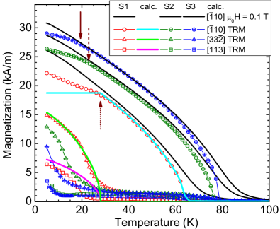
Figure 2: (Color online) Temperature dependence of remnant magnetization components in all three samples (points). Black lines: $M(H)$ at 0.1 T along $[\overline{1}10]$ - the in-plane uniaxial easy axis. Solid lines of lighter shades: the same magnetization components calculated according to a model of only two: uniaxial and biaxial magnetic anisotropies operating at (001) plane and undergoing a spin reorientation transition at temperatures $T^{*}$ (marked by arrows), as in (001) (Ga,Mn)As.

In an analogy to (001) (Ga,Mn)As, let us assume for a moment that $\bm{M}$ of a (113) sample remains (without a magnetic field) in (001) plane. Then, a similar description in terms of two in-plane anisotropies (one biaxial and one uniaxial) is possible. Furthermore, assuming that the uniaxial anisotropy constant is proportional to $M(T)^{2}$, the biaxial anisotropy constant is proportional to $M(T)^{4}$ (Ref. Wang et al., 2005a), and that both equilibrate at $T^{*}$ we are able to model qualitatively temperature induced rotation of magnetization in the sample and calculate all three components of magnetization that would be measured by SQUID. The thick solid lines in Fig. 2 show the results for sample S1 and we find them reproducing the experimental findings reasonably well. Therefore we identify $T^{*}$ as the temperature at which the spin reorientation transition from a biaxial anisotropy along $\langle 100\rangle$ to uniaxial one along $[1\overline{1}0]$ takes place in this system. On the other hand, the discrepancies seen in Fig. 2 indicate that a more elaborated model is needed. In particular, we can infer from the low temperature TRM data that the orientation of $\bm{M}$ at 5 K moves actually away from $\langle 100\rangle$ on annealing. The angle between $\bm{M}$ and $\langle 100\rangle$ is increasing from 9, through 19 to 26 deg for samples S1, S2 and S3 respectively. At the same time the angle between $\bm{M}$ and (113) plane is dropping from 13 to 7 deg. This indicates that the plane in which both easy orientations of $\bm{M}$ reside at low $T$ is tilting away from (001) towards (113) plane. This observation is fully confirmed from the comprehensive analysis of the magnetic anisotropy presented in the next section.

We remark here that the origin of the symmetry breaking between $[110]$ and $[1\overline{1}0]$ in (001) (Ga,Mn)As is still unknown and it is very stimulating to see favoring the in-plane $[1\overline{1}0]$ also in layers of different surface reconstruction than (001) GaAs.

III.2 Experimental determination of anisotropy constants

In order to build up a more complete anisotropy description we analyze full magnetization curves $M(H)$. It was shown by Limmer et al. (Ref. Limmer et al., 2006b, a) that an accurate description the magnetic anisotropy in (113)A (Ga,Mn)As requires at least four components: a cubic magnetic anisotropy with respect to the $\langle 001\rangle$ axes, uniaxial in-plane anisotropy along the $[\overline{1}10]$ direction, and two uniaxial out-of-plane anisotropies along the $[113]$ and $[001]$ directions. The first two anisotropy components are commonly observed in (001)-oriented (Ga,Mn)As samples, and as shown in the previous section they are sufficient to provide even semi-quantitative description in (113) case. The other two arise from the epitaxial strain and demagnetizing effect, both of which depend on the orientation of the substrate. In our approach we combine the two out-of-plane magnetic anisotropy contributions into a single one, with its hard axis oriented between the $[001]$ and $[113]$ directions. Accordingly, we write the free energy in the form,

$$F = -\mu_{0}\bm{H}\cdot\bm{M}+K_{C}(w_{x}^{2}w_{y}^{2}+w_{y}^{2}w_{z}^{2}+w_{z}^{2}w_{x}^{2})$$ (1)

$${}+K_{u\overline{1}10}\sin^{2}\Theta\sin^{2}\Phi$$

$${}+K_{u1}(\cos\Theta_{A}\cos\Theta-\sin\Theta_{A}\sin\Theta\cos\Phi)^{2}.$$

Here, $K_{C}$, $K_{u\overline{1}10}$ and $K_{u1}$ are the lowest order cubic, in-plane uniaxial and out-of-plane uniaxial anisotropy energies, respectively; $\Theta_{A}$ describes the angle between the $K_{u1}$ hard axis and $[113]$ direction; $w_{x}$, $w_{y}$, and $w_{z}$ denote direction cosines of the magnetization vector with respect to the main crystallographic directions $\langle 100\rangle$; $\Theta$ is the angle between $\bm{M}$ and the $[113]$ direction, and $\Phi$ is the angle between the projection of the $\bm{M}$ onto the sample plane and the $[33\overline{2}]$ direction.

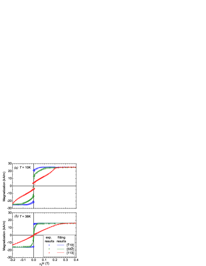
Figure 3: (Color online) Examples of magnetization curves for the as-grown sample measured along three, mutually orthogonal, major sample directions $[\overline{1}10]$, $[33\overline{2}]$, and $[113]$: (a) below spin reorientation transition at 10 K and (b) above, at 38 K. Symbols indicate measurement points; lines represent the best fit of the model described by Eq. (1).

By numerical minimizing of the free energy with respect to $\Theta$ and $\Phi$ we are able to trace the rotation of $\bm{M}$, starting from the given orientation, while sweeping or rotating external magnetic field. Adjusting the obtained “trace” to the experimental data we get the values of the four parameters of the model. We perform this procedure numerically for every sample for all three orientations and for all temperatures the $M_{i}(H)$ curves have been recorded. Figure 3 shows an example of the measured and fitted $M_{i}(H)$ for the sample S1 at two different temperatures.

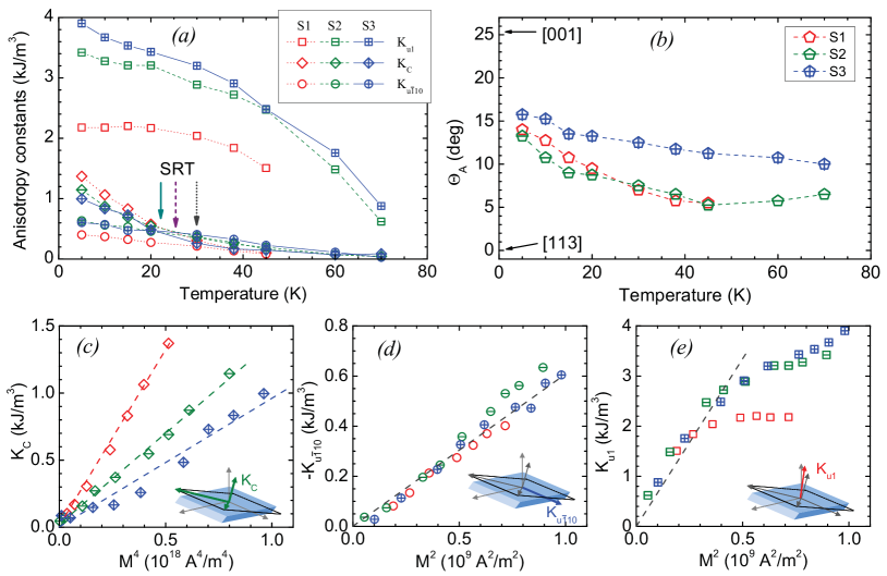
Figure 4: (Color online) (a) and (b) points: temperature dependence of $K_{C}$, $K_{u\overline{1}10}$ and $K_{u1}$ (a) and angle $\Theta_{A}$ (b) obtained from numerical fitting of Eq. (1) to experimental magnetization curves for all three samples considered in this study. Solid, dashed and dotted arrows in (a) indicate the spin reorientation temperature in samples S1, S2 and S3, respectively. (c), (d) and (e): $K_{C}$, $K_{u\overline{1}10}$ and $K_{u1}$ dependence on $M^{4}$, $M^{2}$ and $M^{2}$, respectively. In all panels, the various lines are guides for eye only.

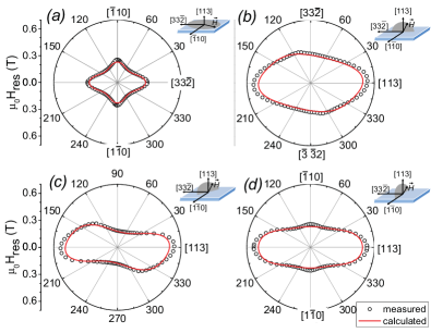
Figure 5: (Color online) Angular dependence of the ferromagnetic resonance fields for external magnetic field rotating in four different crystallographic planes: $(113)$, $(\overline{1}10)$, $(33\overline{2})$ and $\frac{1}{2\sqrt{11}}(3-\sqrt{11},3+\sqrt{11},-2)$. Points show measured resonance field values. Lines show resonant field values calculated using anisotropy energy described by Eq. (1) and magnetic anisotropy constants obtained from hysteresis loops.

Temperature dependence of the three magnetic anisotropy constants and the angle $\Theta_{A}$ are presented in Fig. 4a and b, respectively. All $K_{i}$’s monotonically decrease with temperature, and, like in (001) (Ga,Mn)As, the cubic anisotropy constant $K_{C}$ (with $\langle 100\rangle$ easy axes, see Fig. 4c) and in-plane uniaxial constant $K_{u\overline{1}10}$ (with $[1\overline{1}0]$ easy axis, see Fig. 4d) are proportional to $M^{4}$ and $M^{2}$, respectively, so confirming the validity of the single domain approach used to analyze the observed magnetization rotations. The $K_{C}(T)$ and $K_{u\overline{1}10}(T)$ data point to the presence of the spin reorientation transition in (001) plane. This already inferred from TRM data magnetic easy axis changeover must take place as $K_{C}(T)$ and $K_{u\overline{1}10}(T)$ swap their intensities in our samples. The relevant temperatures are marked in Fig. 4a by arrows. Importantly, we find these temperatures to agree within 2-3 K with those indicated in Fig. 2, what strongly underlines the correctness of the approach we employ here to describe the magnetic anisotropy in our samples. We note that the SRT shifts to lower temperatures on going from sample S1 to S3, since on annealing the in-plane uniaxial anisotropy gets strongly enhanced relative to the cubic one (compare Figs. 4c and d).

In contrast, $K_{u1}$ shows a more complex dependence on $M^{2}$, see Fig. 4e. A proportionality of the out-of-plane anisotropy constant to $M^{2}$ is seen only at low $M$, that is at high $T$. On lowering temperature $K_{u1}$ departures from this trend, and the effect is the strongest for the sample S1. We connect this behavior with the proximity of this system to another spin reorientation transition, the transition from the hard to easy out-of-plane axis of the $K_{u1}$ uniaxial magnetic anisotropy. Such a SRT takes place in compressively strained (001) (Ga,Mn)As on lowering $T$, and was already observed in samples with moderate or high $x$ but rather low hole densitySawicki et al. (2004). The effect depends on the ratio of valence band spin splitting to the Fermi energy. Therefore the S1 sample, the one with the lowest $p$ is expected to show the strongest deviations from the expected functional form. Then on annealing, along with the increase of $p$, we expect the so called in-plane magnetic anisotropy (for the compressively strained layers) to become more robust [less dependent on the magnitude of the valence band splitting, that is on $M(T)$], as experimentally observed.

Finally, we comment on $\Theta_{A}$, the parameter that can serve as a measure of the angle between an ‘easy plane’ with respect to $K_{u1}$ (perpendicular) hard axis and the sample face. As indicated in Fig. 4b that angle remains nearly constant at elevated temperatures and shows a weak, but noticeable turn towards [001] below temperatures which can be associated with $K_{u\overline{1}10}\Leftrightarrow K_{C}$ SRT. This behavior again indicates the departure of easy direction of $\bm{M}$ from $[1\overline{1}0]$ direction in the (113) plane. However, the maximum determined value of $\Theta_{A}\cong 15^{o}$ indicates, that the rotation of $\bm{M}$ actually neither takes place in the (001) plane, nor is it directed exactly towards $\langle 100\rangle$ directions. $\bm{M}$ rather follows a complex route in between (001) and (113) planes, a conclusion that is a numerical confirmation of the results of the simple analysis of the TRM data presented in the previous section.

III.3 Ferromagnetic resonance

A tool widely used to study magnetic anisotropy is ferromagnetic resonance spectroscopy. Magnetic anisotropy in thin (Ga,Mn)As films on (113)A GaAs was recently studied by BihlerBihler et al. (2006) and LimmerLimmer et al. (2006b, a). In a ferromagnetic resonance experiment the magnetization vector $\bm{M}$ of the sample precesses around its equilibrium direction in given external magnetic field $\bm{H}$ with Larmor frequency $\omega_{L}$. The resonant condition at a fixed frequency of microwaves $\omega$ is given by,

$$\left(\frac{\omega}{\gamma}\right)^{2}=\frac{1}{\sin^{2}\Theta}\left[\frac{\partial^{2}F}{\partial\Theta^{2}}\frac{\partial^{2}F}{\partial\Phi^{2}}-\left(\frac{\partial^{2}F}{\partial\Theta\,\partial\Phi}\right)^{2}\right].$$ (2)

Here, $\gamma=g\mu_{B}\hbar^{-1}$ is the gyromagnetic ratio, $g$ is the $g$-factor, $\mu_{B}$ the Bohr magneton, and $\hbar$ is the Planck constant. Resonance field is obtained by evaluating Eq. (2) at the equilibrium position of $\bm{M}$ ($\partial F/\partial\Theta=0$ and $\partial F/\partial\Phi=0$).

In Fig. 5 the dependence of the measured resonant fields on the orientation of the applied magnetic field is shown for the sample S2, along with the results of a calculation made according to Eq. (2) with the magnetic anisotropy parameters obtained from SQUID magnetization curves. The agreement between the calculation and the measured data is very good, indicating that Eq. (1) captures main features of magnetic anisotropy and that the numerical procedure employed to extract the anisotropy constants is correct.

III.4 Magnetization reversal

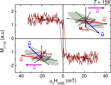
Figure 6: (Color online) The out-of-plane magnetization component dependence on the in-plane magnetic field (swept along $[33\overline{2}]$). The measurement is performed on the as-grown sample S1 at $T=15$ K. The cartoons inserted in the figure illustrate the process.

We end the experimental part evidencing an interesting mechanism of the reversal of the out-of-plane magnetization component by an in-plane magnetic field.

Below the spin reorientation transition (about 20-30 K) the magnetization easy axes are moving close to the $\langle 100\rangle$ directions, that is they are tilted up from the sample face, the (113) plane, and so $\bm{M}$ is acquiring a sizable non-zero component $M_{[113]}$. These two axes define a plane lying between (113) and (001) planes, which shares the common $[\overline{1}10]$ direction with those two planes. Therefore, any sweep of an external field, except that along the $[\overline{1}10]$ direction, will result in a magnetization rotation across the $[\overline{1}10]$ line from one half of that plane (say that one ‘above’ sample face) to the other one (say ‘below’) resulting in $M_{[113]}$ reversal.

Such a process is illustrated in Fig. 6 in the most interesting case, when the field is swept in the sample plane, along $[33\overline{2}]$. We record the $M_{[113]}$ magnetization component using the polar MOKE technique and a clear change of sign of the signal evidences the reversal of $\bm{M}$ by the application of an in-plane magnetic field. The cartoons inserted in this figure visualize the mechanism of this reversal.

IV Theory of magnetic anisotropy

IV.1 $\bm{k}\cdot\bm{p}$ Hamiltonian

The current theory describing the properties of the (Ga,Mn)As ferromagnetic semiconductor is the $p$-$d$ Zener model.Dietl et al. (2000) In this model, the thermodynamic properties are determined by the valence band carriers contribution to the free energy of the system, which is calculated taking the spin-orbit interaction into account within the $\bm{k}\cdot\bm{p}$ theoryDietl et al. (2000, 2001); Jungwirth et al. (2006); Zemen et al. (2009) or tight binding modelWerpachowska and Dietl (2009) with the $p$-$d$ exchange interaction between the carriers and the localized Mn spins considered within the virtual-crystal and molecular-field approximations. Within this approach, magnetic anisotropy depends on the strain tensor components.

The 6-band Luttinger $\bm{k}\cdot\bm{p}$ Hamiltonian of a valence band electron in a zinc-blende semiconductor is a block matrix (cf. Ref. Śliwa and Dietl, 2006):

$$\mathcal{H}_{\mathrm{6x6}}=\begin{pmatrix}H^{vv}&H^{vs}\\ H^{sv}&H^{ss}\end{pmatrix},$$ (3)

where

$$\mathcal{H}^{vv} = -\frac{\hbar^{2}}{m}\left\{\frac{1}{2}\gamma_{1}k^{2}-\gamma_{2}\left[\left(J_{x}^{2}-\frac{1}{3}J^{2}\right)k_{x}^{2}+c.p.\right]\right.$$

$$\left.{}-2\gamma_{3}\left[\{J_{x},J_{y}\}\{k_{x},k_{y}\}+c.p.\right]\right\}$$

$$\mathcal{H}^{vs} = -\frac{\hbar^{2}}{m}\left[-3\gamma_{2}(U_{xx}k_{x}^{2}+c.p.)\right.$$

$$\left.{}-6\gamma_{3}(U_{xy}\{k_{x},k_{y}\}+c.p.)\right]$$

$$\mathcal{H}^{ss} = -\left(\Delta_{0}+\frac{\hbar^{2}}{2m}\gamma_{1}k^{2}\right)$$ (6)

(we use the notation of Ref. Śliwa and Dietl, 2006). Our basis is related to that of Ref. Dietl et al., 2001 as follows: $u_{1}=-\left|\frac{3}{2},\frac{3}{2}\right>$, $u_{2}=-i\left|\frac{3}{2},\frac{1}{2}\right>$, $u_{3}=\left|\frac{3}{2},-\frac{1}{2}\right>$, $u_{4}=i\left|\frac{3}{2},-\frac{3}{2}\right>$, $u_{5}=-\left|\frac{1}{2},\frac{1}{2}\right>$, $u_{6}=i\left|\frac{1}{2},-\frac{1}{2}\right>$, i.e. we use the standard basis of angular momentum eigenvectors (notice the change of sign in $\left|\frac{1}{2},\frac{1}{2}\right>$ and $\left|\frac{1}{2},-\frac{1}{2}\right>$ with respect to Ref. Śliwa and Dietl, 2006 that accounts for the difference in the sign of $H^{vs}$, $H^{sv}$). In this basis the $p-d$ exchange Hamiltonian is:

$$\mathcal{H}_{pd}=B_{G}\begin{pmatrix}2(\bm{J}\cdot\bm{w})&-6(\bm{U}\cdot\bm{w})\\ -6(\bm{T}\cdot\bm{w})&-(\bm{\sigma}\cdot\bm{w})\end{pmatrix},$$ (7)

where $\bm{w}=\bm{M}/M$ and $B_{G}$ is given by equation 2 of Ref. Dietl et al., 2001,

$$B_{G}=A_{F}\beta M/(6g\mu_{B}),$$ (8)

while the strain Hamiltonian is:

$$\mathcal{H}^{vv}_{\epsilon} = -b\Bigl{[}(J_{x}^{2}-\frac{1}{3}J^{2})\epsilon_{xx}+c.p.\Bigr{]}$$ (10)

$${}-\frac{d}{\sqrt{3}}\Bigl{[}2\{J_{x},J_{y}\}\epsilon_{xy}+c.p.\Bigr{]}$$

$$\mathcal{H}^{vs}_{\epsilon} = -3b(U_{xx}\epsilon_{xx}+c.p.)$$ (12)

$${}-\sqrt{3}d(2U_{xy}\epsilon_{xy}+c.p.)$$

$$\mathcal{H}^{ss}_{\epsilon} = 0.$$ (13)

Since the strain tensor for the $(113)$ substrate orientation features non-zero non-diagonal components, it is necessary to include in the $\bm{k}\cdot\bm{p}$ Hamiltonian the so called $k$-linear terms, i.e., terms linear in $\bm{k}$ and $\bm{\epsilon}$ coming via second-order perturbation (Ref. Bir and Pikus, 1974, §15) from the terms in the $8\times 8$ Kane HamiltonianPikus and Titkov (1984) that mix the conduction and the valence bands. The corresponding Hamiltonian is

$$\mathcal{H}_{k\epsilon}=C_{4}\begin{pmatrix}\bm{J}\cdot\bm{\varphi}&\frac{3}{2}\left(1-\frac{\eta}{2}\right)\bm{U}\cdot\bm{\varphi}\\ \frac{3}{2}\left(1-\frac{\eta}{2}\right)\bm{T}\cdot\bm{\varphi}&\left(1-\eta\right)\bm{\sigma}\cdot\bm{\varphi}\end{pmatrix},$$ (14)

where $\eta=\Delta_{0}/(E_{g}+\Delta_{0})$ and the components of the vector $\bm{\varphi}$ are $\varphi_{z}=\epsilon_{zx}k_{x}-\epsilon_{zy}k_{y}$ (c.p.). The numerical value given in Ref. Pikus and Titkov, 1984 is $C_{3}/\hbar=8\times 10^{5}\,\mathrm{m}\,\mathrm{s}^{-1}$, hence for $C_{4}=-C_{3}/(2\eta)$ we obtain $C_{4}/\hbar=-2.2\times 10^{6}\,\mathrm{m/s}$.

IV.2 Strain tensor

Determining the components of the strain tensor for an unrelaxed epitaxial layer grown on a lattice mismatched substrate can be considered a classical topic. The two possible approaches to this problem are (i) to solve a system of linear equations for the strain and stress components assuming that some components of those tensors vanish (this is our approach) or (ii) to determine the strain of the layer by minimizing the elastic energy (this is the approach formulated in Ref. Yang et al., 1994). Our approach involves a transformation of the coordinate system that is feasible in general only using a computer algebra system. Using one we arrive to the form of the symmetric strain tensor that is in a perfect agreement with that of Ref. Yang et al., 1994.

The result for a $(11n)$ oriented substrate is,

$$\bm{\epsilon}_{\text{epi}}=\frac{f}{A+B+C}\begin{pmatrix}B+C&-A&-D/2\\ -A&B+C&-D/2\\ -D/2&-D/2&B-2C\end{pmatrix},$$ (15)

where

$$A = 3\left[n^{2}(c_{11}-c_{12})-(n^{2}-2)c_{44}\right](c_{11}+2c_{12}),$$ (16)

$$B = 2\left[(n^{4}+4n^{2}+1)(c_{11}-c_{12})+6c_{44}\right]c_{44},$$ (17)

$$C = (n^{2}-1)(n^{2}+2)(c_{11}+2c_{12})c_{44},$$ (18)

$$D = 3n\left[(n^{2}+1)(c_{11}-c_{12})+2c_{44}\right](c_{11}+2c_{12}),\quad$$ (19)

and

$$f=-\Delta a/a=(a_{0}-a)/a$$ (20)

is the relative lattice constant misfit. Here, the components of the epitaxial strain tensor are given with respect to the coordinates $(x,y,z)$ associated with the crystallographic axes, $x=[100]$, $y=[010]$, and $z=[001]$ (i.e. the quantities given above are the strain components that enter the $\bm{k}\cdot\bm{p}$ Hamiltonian).

Using the values $c_{11}=119.\,\mathrm{GPa}$, $c_{12}=53.8\,\mathrm{GPa}$, and $c_{44}=59.5\,\mathrm{GPa}$ (Ref. Madelung, 1991, p. 105) we obtain

$$\bm{\epsilon}_{\text{epi}}=-\frac{\Delta a}{a}\begin{pmatrix}\phantom{-}0.9488&-0.0512&-0.3478\\ -0.0512&\phantom{-}0.9488&-0.3478\\ -0.3478&-0.3478&-0.6260\end{pmatrix}.$$ (21)

For the purpose of determining the strain components from X-ray diffraction data, the components of the strain tensor in the coordinate system associated with the epitaxial film are needed. We take as the coordinate system: $x^{\prime}=[3,3,-2]$, $y^{\prime}=[-1,1,0]$, $z^{\prime}=[1,1,3]$. The relative difference of the lattice constants along the $[113]$ direction between that layer and the substrate is

$$\Delta d/d = \frac{[27(c_{11}-c_{12})+67c_{44}](c_{11}+2c_{12})}{9(c_{11}-c_{12})(c_{11}+2c_{12})+(101c_{11}-34c_{12}+4c_{44})c_{44}}\Delta a/a=1.7284\,\Delta a/a.$$ (22)

For the sake of completeness we notice that there is also a shear strain component

$$\epsilon_{x^{\prime}z^{\prime}} = \frac{12\sqrt{2}[(c_{11}-c_{12})-2c_{44}](c_{11}+2c_{12})}{9(c_{11}-c_{12})(c_{11}+2c_{12})+(101c_{11}-34c_{12}+4c_{44})c_{44}}\Delta a/a=-0.2746\,\Delta a/a.$$ (23)

Following Ref. Sawicki et al., 2005, to account for the mechanism which generates the in-plane uniaxial anisotropy in $(001)$ samples, we incorporate in the $p-d$ Zener model an additional Hamiltonian term corresponding to shear strain $\bm{\epsilon}^{\prime}$,

$$\bm{\epsilon}=\bm{\epsilon}_{\text{epi}}+\bm{\epsilon}^{\prime}.$$ (24)

In case of a $(001)$-oriented substrate the additional strain $\bm{\epsilon}^{\prime}$ has a non-zero $xy$ component, $\epsilon^{\prime}_{xy}$. The corresponding anisotropy is of the form $K_{xy}w_{x}w_{y}$ (as in Ref. Bowden et al., 2008), hence it is a difference of uniaxial anisotropies on the $[110]$ and $[\overline{1}10]$ directions, and the anisotropy field is $H_{u}=2K_{xy}/(\mu_{0}M)$ (this is the field required to align magnetization along the hard axis, e.g. $[110]$; only $H_{u}/2$ is required to align magnetization along the $z$ direction). In the case of a $(113)$-oriented substrate the additional strain may have more non-zero components. We assume that the mirror symmetry with respect to the $(\overline{1}10)$ plane is preserved, hence $\epsilon^{\prime}_{xz}=\epsilon^{\prime}_{yz}$.

IV.3 Numerical procedure

The numerical procedure serving to determine the magnetic anisotropy from the Hamiltonian matrix is described in Ref. Dietl et al., 2001. Let us note that including the $k$-linear terms in the Hamiltonian leads to a tenfold increase of the processing time, although in specific cases it is possible to generate a symbolic expression for the characteristic polynomial of the $6\times 6$ Hamiltonian matrix. Moreover, since numerical interpolation of the dependence of the hole concentration on the Fermi energy may lead to uncontrollable inaccuracies, an alternative procedure that avoids those inaccuracies is to directly integrate the energy of the carriers in the momentum space. However, the integration has to be done separately for each hole concentration (this is an advantage if a single hole concentration is specified). Moreover, one still needs to solve the inverse eigenvalue problem to find the discontinuities of the integrand.

In a numerical calculation, it is possible to determine the full magnetic anisotropy by computing the free energy of the carriers for a number of directions of magnetization. In our case we choose a grid of directions that is rectangular in the spherical coordinates ($w_{x}=\sin\theta\cos\phi$, $w_{y}=\sin\theta\sin\phi$, $w_{z}=\cos\theta$), i.e. $\theta=\theta_{i}$ and $\phi=\phi_{j}$, where $\cos\theta_{i}$, $i=1,2,\ldots,N_{\theta}$ are the nodes of a Gaussian quadrature and $\phi_{j}=2\pi j/N_{\phi}$, $j=0,1,\ldots,N_{\phi}-1$ are equally spaced. Then, following the method used in the software package SHTOOLSWieczorek (routine SHExpandGLQ) we expand the magnetic anisotropy (free energy) into a sum of low-order spherical harmonics. Since the free energy is even, choosing even $N_{\phi}$ allows to restrict the grid to a half of the sphere. We use the standard quantum mechanics (orthonormalized) spherical harmonics $Y_{lm}(\theta,\phi)$, and denote the coefficients of this expansion $r_{lm},m=0,1,\ldots,l$, and $s_{lm},m=1,2,\ldots l$,

$$F_{c}=\sum_{l}\left[r_{l0}Y_{l0}+\sum_{m=1}^{l}(r_{lm}\Re Y_{lm}+s_{lm}\Im Y_{lm})\right],$$ (25)

where the outer sum is over $l=0,2,\ldots,N_{\theta}-1$. The scalar product in this representation is diagonal, with a weight of $1$ for $r_{l0}$ and $1/2$ for $r_{lm}$, $s_{lm}$, $m>0$.

IV.4 Magnetic anisotropy

There are a few sources of magnetic anisotropy in epitaxial $\mathrm{Ga}_{1-x}\mathrm{Mn}_{x}\mathrm{As}$: the cubic anisotropy of the valence band, epitaxial strain, the additional off-diagonal strain $\epsilon^{\prime}$, and the shape anisotropy caused by the demagnetization effect. Since $\epsilon^{\prime}$ is unknown, it is inevitable to parametrize the anisotropy in a manner that separates the components affected by $\epsilon^{\prime}$ from what is predictable. If we measure $(\theta,\phi)$ in the spherical harmonic representation of the carriers’ free energy with respect to the crystallographic axes, the above spherical harmonic representation allows one to separate the components brought about by a non-zero value of $\epsilon^{\prime}$ from the remaining sources of magnetic anisotropy. Indeed, as far as $l=2$ is concerned, $\epsilon^{\prime}$ affects primarily only $K_{xy}$, $K_{yz}$, and $K_{xz}$, where $K_{xy}=\sqrt{\frac{15}{8\pi}}s_{22}$, $K_{yz}=-\sqrt{\frac{15}{8\pi}}s_{21}$, and $K_{xz}=-\sqrt{\frac{15}{8\pi}}r_{21}$. The remaining components are $r_{20}$ and $r_{22}$. As $r_{22}=0$ due to the mirror symmetry, they can be collected into one term $K_{u001}(w_{z}^{2}-\frac{1}{3})$, with $K_{u001}=\frac{3}{4}\sqrt{\frac{5}{\pi}}r_{20}$. Thus, we describe the $l=2$ anisotropy (without the demagnetization contribution) by $K_{xy}$, $K_{xz}=K_{yz}$, and $K_{u001}$. Finally, the cubic anisotropy corresponds to $(r_{40},r_{44})=-\frac{2\sqrt{\pi}}{15}K_{C}(1,\sqrt{10/7})$.

We have to relate now the components of the spherical harmonic representation, $r_{lm}$ and $s_{lm}$, to the experimentally determined magnetic anisotropy constants $K_{C},K_{u1},K_{u\overline{1}10}$, and $\Theta_{A}$, as specified in Eq. 1 and presented in Fig. 4. Since the demagnetization effect adds to $(r_{20},r_{21},s_{21},r_{22},s_{22})$ the contribution $\frac{4\sqrt{10\pi}}{165}K_{d}(4\sqrt{2},-3\sqrt{3},-3\sqrt{3},0,\sqrt{3})$, with $K_{d}=\mu_{0}M^{2}/2$, the constants are related to those of Eq. (1) as follows,

$$K_{u001} = \frac{1+3\cos 2\Theta_{A}^{\prime}}{4}K_{u1}-\frac{1}{2}K_{u\overline{1}10}-\frac{8}{11}K_{d},\quad$$ (26)

$$K_{xy} = \frac{1-\cos 2\Theta_{A}^{\prime}}{2}K_{u1}-K_{u\overline{1}10}-\frac{2}{11}K_{d},$$ (27)

$$K_{xz} = -\frac{\sqrt{2}\sin 2\Theta_{A}^{\prime}}{2}K_{u1}-\frac{6}{11}K_{d},$$ (28)

where $\Theta_{A}^{\prime}=\Theta_{A}-\arccos(3/\sqrt{11})$.

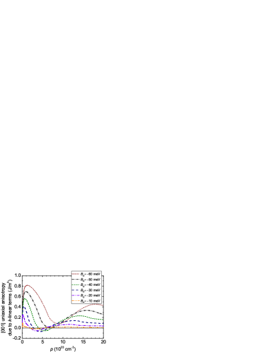
Figure 7: (Color online) The contribution of the $k$-linear terms to the $[001]$ uniaxial anisotropy for $C_{4}/\hbar=-2.18\times 10^{6}\,\mathrm{m/s}$ and $\epsilon_{xy}=0.05\%$.

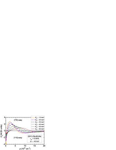
Figure 8: (Color online) Hole concentration dependence of the in-plane uniaxial anisotropy field due to shear strain $\epsilon_{xy}=0.05\%$ for various values of the valence-band spin-splitting.

We carry out numerical calculations with band structure parameters and deformation potentials specified previously.Dietl et al. (2001); Sawicki et al. (2005) We include hole-hole exchange interactions via the Landau parameter of the susceptibility enhancement, $A_{F}=1.2$ (Ref. Dietl et al., 2001). This parameter, assumed here to be independent of the hole density and strain, enters into the relation between $M$ and $B_{G}$, but also divides the anisotropy constants. More specifically, we make the calculation with $B_{G}$ enhanced by the factor $A_{F}$, and divide the resulting anisotropy constants by $A_{F}^{n-1}$, where $n$ is the power of magnetization $M$ to which a given anisotropy constant is proportional. The result is proportional to $A_{F}$. We have $n=2$ for the uniaxial anisotropies and $n=4$ for the lowest order cubic anisotropy (the proportionality holds for $B_{G}$ smaller than a few meV). We note that the cubic anisotropy field shown in Fig. 9 of Ref. Dietl et al., 2001 was divided by $A_{F}$ rather than $A_{F}^{3}$.

To evaluate the effect of the $k$-linear terms, we use a non-zero value of $C_{4}$ and calculate the difference of the resulting anisotropy with respect to the $C_{4}=0$ case. This difference has only one noticeable component, $\Delta r_{20}=r_{20}(C_{4}\neq 0)-r_{20}(C_{4}=0)$, which corresponds to a uniaxial anisotropy with a $[001]$ axis (or with $[100]$, $[010]$ axes for $\epsilon_{yz}\neq 0$, $\epsilon_{xz}\neq 0$ respectively). A plot of $\Delta K_{u001}\propto\Delta r_{20}$ is shown in Fig. 7 for $\epsilon_{xy}=0.05\%$ (as implied by the symmetry, $\Delta K_{u001}$ is second order in $\epsilon_{xy}$). The values are rather small. In fact, assuming $\Delta a/a=0.5\%$, we have $\epsilon_{xz}=\epsilon_{yz}\approx 0.17\%$, and the magnitude of $\Delta K_{u100}=\Delta K_{u010}$ is below $10\,\mathrm{J}/\mathrm{m}^{3}$ if we consider the epitaxial strain only. This estimate appears to remain valid in case of a general strain of a similar magnitude, although other anisotropy components are affected as well and the dependence on strain components is non-linear. However, we stress that this estimate depends on the value of the parameter $C_{4}$, which is somewhat uncertain and may be different for the ordinary strain and $\bm{\epsilon}^{\prime}$. Considered this, it is justified to set $C_{4}=0$ in the remaining part of this paper.

Before we proceed to the calculations specific to the particular samples, we make a remark that the data originally shown in Fig. 6 of Ref. Sawicki et al., 2005 were not correct due to a numerical error in the form of the strain Hamiltonian. We show corrected results for $H_{u}$ in Fig. 8. The present results are in agreement with Fig. 17 of Ref. Zemen et al., 2009 (remember that our model includes the parameter the Landau parameter $A_{F}$, neglected in Ref. Zemen et al., 2009).

As discussed previously,Sawicki et al. (2004, 2005) owing to sign oscillations of anisotropy constants, the direction of magnetization can be changed by temperature ($B_{\text{G}}$) or the hole concentration, particularly in the vicinity of $p=6\times 10^{20}$ and $1\times 10^{20}$ cm^-3, according to the results displayed in Fig. 8 The corresponding in-plane spin reorientation transition has indeed been observed by some of us either as a function of temperatureSawicki et al. (2005) or the gate voltage in metal-insulator semiconductor structuresChiba et al. (2008); Sawicki et al. (2010) in these two hole concentration regions in (Ga,Mn)As, respectively.

V Comparison between experiment and theory

We detailed above a microscopic model of the magnetic anisotropy in a DMS. In order to assess the applicability of this model to an arbitrarily oriented DMS we compare its predictions with experimental findings for (113) (Ga,Mn)As.

First, we specify the magnitude of the lattice mismatch to establish the components of the strain tensor. According to Fig. 2 of Ref. Daeubler et al., 2006, for a $(113)$ sample containing 6.4% of Mn we expect $\Delta d/d=5.6\times 10^{-3}$ which, employing Eq. 22, translates into $\Delta a/a=0.323\%$. We assume this value throughout this section.

Then, using the values of $x_{\text{eff}}$ already established in Sec. II, we calculate

$$M_{\text{Mn}}=x_{\text{eff}}N_{0}Sg\mu_{B}$$ (29)

and obtain $B_{G}$ for each of our samples from Eq. 8. It is worth repeating here, that the established upon total $x$ and $M_{\text{exp}}$ values of $x_{\text{eff}}$ and $p$ reproduce, within the same model, experimental values of $T_{\text{C}}$ remarkably well. This boosts our confidence in the accuracy of the material parameters used here for the computations of the magnetic anisotropy and gives a solid ground to the presented conclusions.

The calculations are performed as a function of $p$, employing for each sample the corresponding value of $B_{G}$: $-16.4$, $-18.7$, and $-19.7$ meV for samples S1, S2, and S3, respectively. The results are presented in Fig. 9 as curves, while full symbols represent experimentally established values of the anisotropy constants (a square for the sample S1, a triangle for S2, and a circle for S3). The experimental $K_{u001}$, $K_{xy}$, $K_{xz}$, and $K_{C}$ are obtained from $K_{u\overline{1}10}$, $K_{u1}$, $K_{C}$ and $\Theta_{A}$ using Eqs. 26, 27 and 28. We take the $T=5\,\mathrm{K}$ experimental anisotropy data, as this is what is consistent with the $T=0$ limit, implicitly assumed in Eq. 29.

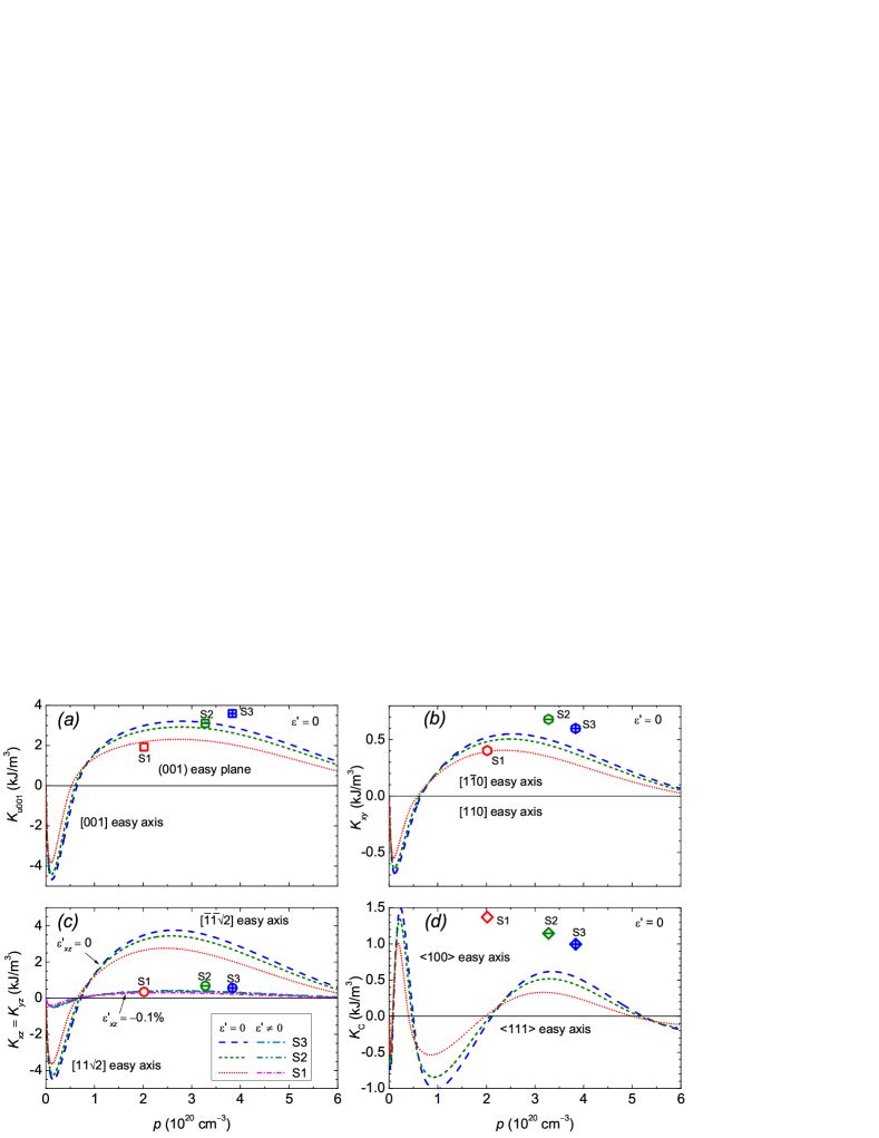
Figure 9: (Color online) Lines: theoretical dependence of the anisotropy constants (a) $K_{u001}$, (b) $K_{xy}$, (c) $K_{xz}$, and (d) $K_{C}$ on the hole concentration $p$, calculated within mean-field Zener model. The values of the exchange parameter $B_{G}$ and the lattice constant mismatch $\Delta a/a$ are specific to the investigated samples and are specified in the text. Symbols depict values determined from the experiment. $\bm{\epsilon}^{\prime}=0$ is assumed here except for (c), where also the case of $\epsilon^{\prime}_{xz}=-0.1\%$ is included.

We start by discussing the strongest component of the magnetic anisotropy, the $K_{u001}$ term. The calculated curves are presented in Fig. 9a. The calculations have been performed without introducing the fictitious shear strain $\bm{\epsilon}^{\prime}$ (i.e. $\epsilon^{\prime}=0$). However, since we know that the magnitude of $K_{u001}$ is negligibly affected by $\bm{\epsilon}^{\prime}$, the results should already match the experimental data, and indeed they do. Although the spread of the experimental points in Fig. 9a is significantly larger than that of the theoretical curves, the correspondence between the computed and experimental values is good, and it has been achieved without introducing into the model any adjustable parameters. This has been only possible by including the hole liquid magnetization in the calculation of $x_{\text{eff}}$. When $M_{h}$ is disregarded, the experimental values of $K_{u001}$ are systematically above the maxima of the theoretical curves.

As already mentioned, in the case of the (001) (Ga,Mn)As films an additional low-symmetry term has to be introduced into the Hamiltonian in order to reproduce the experimentally observed uniaxial in-plane magnetic anisotropy. In a general case of an arbitrarily oriented substrate, there are three anisotropy constants of this kind, $K_{xy}$, $K_{yz}$, and $K_{xz}$. In the case of (113) (Ga,Mn)As, the symmetry requires that $K_{xz}=K_{yz}$, the assumption confirmed by the description of the experimental results. The two relevant anisotropy constants $K_{xy}$ and $K_{xz}$ are presented in Figs. 9(b) and (c), and are seen to be non-zero even in the absence of a symmetry lowering perturbation, $\epsilon^{\prime}_{xy}=0$. The computed magnitude of $K_{xy}$ for $\epsilon^{\prime}_{xy}=0$ yields an acceptable agreement with the experimental data. We note, moreover, that an exact match is possible when allowing for non-zero values of $\epsilon^{\prime}_{xy}\cong 0.001$% for sample S1 and 0.01% for samples S2 and S3.

In contrast, according to Fig. 9(c), the theoretical description of the experimental values of the $K_{xz}$ anisotropy constant requires a quite sizable value of the corresponding strain component $\epsilon^{\prime}_{xz}=-0.1\%$. Thus, remarkably and contrary to the case of (001) (Ga,Mn)As, one barely needs any in-plane shear strain to reproduce in-plane uniaxial anisotropy, whereas for the out-of-plane component two times stronger shear strain is needed comparing to the (001) case. This finding should be taken as a strong evidence that the in-growth surface reconstruction, and a related with it orientational preferences of Mn incorporation must play a decisive role in the mechanism leading to the lowering of magnetic symmetry.

Finally, we turn to the case of the cubic anisotropy constant $K_{C}$, shown in Fig. 9d. Since $K_{C}$ shows only a small sensitivity to $\bm{\epsilon}^{\prime}$, we present the results of computations only for $\bm{\epsilon}^{\prime}=0$. We find that similarly to the (001) case,Sawicki et al. (2004) the present theory underestimates the magnitude of $K_{C}$, particularly in the low hole concentration region, where the theoretically expected change of sign of $K_{C}$ is not observed experimentally. The origin of this discrepancy, and in particular its relation to the symmetry lowering perturbation is presently unknown.

We have also examined theoretically how the particular anisotropy constants depend on magnetization $M$. As could be expected, and in a qualitative agreement with the experimental finding shown in Fig. 4, the uniaxial anisotropy constants $K_{u001}$, $K_{xy}$, and $K_{xz}$ (or equivalently $K_{u1}$ and $K_{u\overline{1}10}$) are proportional to $M^{2}$, whereas $K_{C}$ to $M^{4}$, except to the hole concentration region in the immediate vicinity of the sign change.

VI Conclusions

We have investigated the magnetic properties of as-grown and annealed (Ga,Mn)As layers grown by MBE on GaAs substrates of the $(113)$ orientation and provided the most complete to date description of the magnetic anisotropy in the whole temperature range up to $T_{\mathrm{C}}$. At higher temperatures the $[\overline{1}10]$ direction is the easy magnetization axis before and after annealing. At low temperature the spin reorientation transition to a pair of easy axes near the $[100]$ and $[010]$ directions takes place and to a first approximation, magnetization behavior as a function of temperature is similar to that observed in $(001)$ (Ga,Mn)As in the absence of an external magnetic field.Wang et al. (2005a) However, the magnetization vector resides in a plane close to (001) plane only for a low value of the hole concentration. When it increases, the plane rotates along $[\overline{1}10]$ towards the sample face (113), and the two cubic easy directions move towards the $[33\overline{2}]$ direction.

We have estimated the values of magnetic anisotropy constants by fitting our phenomenological model to the hysteresis loops measured by SQUID. The comparison to results of FMR measurements confirms the correctness of this approach. The obtained values of the cubic and uniaxial in-plane magnetic anisotropy constants are proportional to $M^{4}$ and $M^{2}$, respectively. Inflections from the $M^{2}$ dependence of the out-of-plane uniaxial anisotropy constant indicate a proximity to another spin reorientation transition at which the out-of-plane axis becomes easy on lowering temperature. It has been evidenced by MOKE that it is possible to reverse the out-of-plane magnetization component by applying an in-plane magnetic field.

For the hole and effective Mn concentrations determined from the values of saturation magnetization and the total Mn concentration, the $p-d$ Zener model explains, with no adjustable parameters, the magnitude of the Curie temperature as well as the sign and magnitude of the uniaxial $[001]$ anisotropy constant $K_{u001}$ caused by biaxial strain. At the same time, however, the predicted values of the cubic anisotropy constant are smaller than those found experimentally in the hole concentration range studied here. For the substrate orientation in question there are two additional non-zero second order ($l=2$) components $K_{xy}$ and $K_{xz}$. The comparison of their experimental and theoretical values points to the presence of an additional shear strain. The non-vanishing components of this additional strain are $\epsilon_{xz}^{\prime}=\epsilon_{yz}^{\prime}\approx-0.1$%, in contrast with $(001)$ samples, for which a non-zero value of $\epsilon_{xy}^{\prime}\approx=0.05\%$ has to be assumed in order to explain the experimental data. This finding provides a hint that a preferential Mn incorporation during the growth process accounts for the mysterious lowering of the (Ga,Mn)As symmetry.

References

- Ohno et al. (1996) H. Ohno, A. Shen, F. Matsukura, A. Oiwa, A. Endo, S. Katsumoto, and Y. Iye, Appl. Phys. Lett. 69, 363 (1996).
- Matsukura et al. (2002) F. Matsukura, H. Ohno, and T. Dietl, in Handbook of Magnetic Materials, edited by K. H. J. Buschow (Elsevier, 2002), vol. 14, pp. 1–87.
- Dietl (2008) T. Dietl, in Spintronics, edited by T. Dietl, D. Awschalom, M. Kaminska, and H. Ohno (Elsevier, Amsterdam, 2008), vol. 82 of Semiconductors and Semimetals, p. 371.
- Dietl et al. (2000) T. Dietl, H. Ohno, F. Matsukura, J. Cibert, and D. Ferrand, Science 287, 1019 (2000).
- Dietl et al. (2001) T. Dietl, H. Ohno, and F. Matsukura, Phys. Rev. B 63, 195205 (2001).
- Jungwirth et al. (2006) T. Jungwirth, J. Sinova, J. Mašek, J. Kučera, and A. H. MacDonald, Rev. Mod. Phys. 78, 809 (2006).
- Tang et al. (2003) H. X. Tang, R. K. Kawakami, D. D. Awschalom, and M. L. Roukes, Phys. Rev. Lett. 90, 107201 (2003).
- Welp et al. (2003) U. Welp, V. K. Vlasko-Vlasov, X. Liu, J. K. Furdyna, and T. Wojtowicz, Phys. Rev. Lett. 90, 167206 (2003).
- Sawicki et al. (2004) M. Sawicki, F. Matsukura, A. Idziaszek, T. Dietl, G. M. Schott, C. Rüster, C. Gould, G. Karczewski, G. Schmidt, and L. W. Molenkamp, Phys. Rev. B 70, 245325 (2004).
- Sawicki et al. (2005) M. Sawicki, K.-Y. Wang, K. W. Edmonds, R. P. Campion, C. R. Staddon, N. R. S. Farley, C. T. Foxon, E. Papis, E. Kamińska, A. Piotrowska, et al., Phys. Rev. B 71, 121302(R) (2005).
- Wang et al. (2005a) K. Y. Wang, M. Sawicki, K. W. Edmonds, R. P. Campion, S. Maat, C. T. Foxon, B. L. Gallagher, and T. Dietl, Phys. Rev. Lett. 95, 217204 (2005a).
- Liu et al. (2006) X. Liu, J. K. Furdyna, M. Dobrowolska, W. Lim, C. Xie, and Y. J. Cho, J. Phys.: Condens. Matter 18, R245 (2006).
- Thevenard et al. (2007) L. Thevenard, L. Largeau, O. Mauguin, A. Lemaître, K. Khazen, and H. J. von Bardeleben, Phys. Rev. B 75, 195218 (2007).
- Gourdon et al. (2007) C. Gourdon, A. Dourlat, V. Jeudy, K. Khazen, H. J. von Bardeleben, L. Thevenard, and A. Lemaître, Phys. Rev. B 76, 241301 (2007).
- Gould et al. (2008) C. Gould, S. Mark, K. Pappert, R. G. Dengel, J. Wenisch, R. P. Campion, A. W. Rushforth, D. Chiba, Z. Li, X. Liu, et al., New J. Phys. 10, 055007 (2008).
- Welp et al. (2004) U. Welp, V. K. Vlasko-Vlasov, A. Menzel, H. D. You, X. Liu, J. K. Furdyna, and T. Wojtowicz, Appl. Phys. Lett. 85, 260 (2004).
- Zemen et al. (2009) J. Zemen, J. Kučera, K. Olejník, and T. Jungwirth, Phys. Rev. B 80, 155203 (pages 29) (2009).
- Glunk et al. (2009) M. Glunk, J. Daeubler, L. Dreher, S. Schwaiger, W. Schoch, R. Sauer, W. Limmer, A. Brandlmaier, S. T. B. Goennenwein, C. Bihler, et al., Phys. Rev. B 79, 195206 (pages 10) (2009).
- Wang et al. (2005b) K. Y. Wang, K. W. Edmonds, L. X. Zhao, M. Sawicki, R. P. Campion, B. L. Gallagher, and C. T. Foxon, Phys. Rev. B 72, 115207 (2005b).
- Limmer et al. (2006a) W. Limmer, M. Glunk, J. Daeubler, T. Hummel, W. Schoch, R. Sauer, C. Bihler, H. Huebl, M. S. Brandt, and S. T. B. Goennenwein, Phys. Rev. B 74, 205205 (2006a).
- Limmer et al. (2006b) W. Limmer, M. Glunk, J. Daeubler, T. Hummel, W. Schoch, C. Bihler, H. Huebl, M. S. Brandt, S. T. B. Goennenwein, and R. Sauer, Microelectron. J. 37, 1490 (2006b).
- Pross et al. (2006) A. Pross, S. J. Bending, K. Y. Wang, K. W. Edmonds, R. P. Campion, C. T. Foxon, B. L. Gallagher, and M. Sawicki, J. Appl. Phys. 99, 093908 (pages 6) (2006).
- Bihler et al. (2006) C. Bihler, H. Huebl, M. S. Brandt, S. T. B. Goennenwein, M. Reinwald, U. Wurstbauer, M. Döppe, D. Weiss, and W. Wegscheider, Appl. Phys. Lett. 89, 012507 (2006).
- Liu and Furdyna (2007) X. Liu and J. K. Furdyna, J. Phys.: Condens. Matter 19, 165205 (2007).
- Abolfath et al. (2001) M. Abolfath, T. Jungwirth, J. Brum, and A. MacDonald, Phys. Rev. B 63, 054418 (2001).
- Reinwald et al. (2005) M. Reinwald, U. Wurstbauer, M. Döppe, W. Kipferl, K. Wagenhuber, H.-P. Tranitz, D. Weiss, and W. Wegscheider, J. Cryst. Growth 278, 690 (2005), 13th International Conference on Molecular Beam Epitaxy.
- Yu et al. (2002) K. M. Yu, W. Walukiewicz, T. Wojtowicz, I. Kuryliszyn, X. Liu, Y. Sasaki, and J. K. Furdyna, Phys. Rev. B 65, 201303 (2002).
- Blinowski and Kacman (2003) J. Blinowski and P. Kacman, Phys. Rev. B 67, 121204 (2003).
- Hayashi et al. (2001) T. Hayashi, Y. Hashimoto, S. Katsumoto, and Y. Iye, Appl. Phys. Lett. 78, 1691 (2001).
- Edmonds et al. (2002) K. W. Edmonds, K. Y. Wang, R. P. Campion, A. C. Neumann, N. R. S. Farley, B. L. Gallagher, and C. T. Foxon, Appl. Phys. Lett. 81, 4991 (2002).
- Edmonds et al. (2004) K. W. Edmonds, P. Boguslawski, K. Y. Wang, R. P. Campion, N. R. S. Farley, B. L. Gallagher, C. T. Foxon, M. Sawicki, T. Dietl, M. B. Nardelli, et al., Phys. Rev. Lett. 92, 037201 (2004).
- Wang et al. (2005c) K. Y. Wang, K. W. Edmonds, R. P. Campion, L. X. Zhao, C. T. Foxon, and B. L. Gallagher, Phys. Rev. B 72, 085201 (2005c).
- Kato et al. (2004) H. Kato, K. Hamaya, T. Taniyama, Y. Kitamoto, and H. Munekata, Jpn. J. Appl. Phys. 43, L904 (2004).
- Werpachowska and Dietl (2009) A. Werpachowska and T. Dietl (2009), eprint arXiv:0910.1907.
- Śliwa and Dietl (2006) C. Śliwa and T. Dietl, Phys. Rev. B 74, 245215 (2006).
- Bir and Pikus (1974) G. L. Bir and G. E. Pikus, Symmetry and Strain-Induced Effects in Semiconductors (John Wiley & Sons, New York, 1974).
- Pikus and Titkov (1984) G. E. Pikus and A. N. Titkov, Optical Orientation (North Holland, Amsterdam, 1984), vol. 8 of Modern Problems in Condensed Matter Sciences, chap. 3, pp. 73–131.
- Yang et al. (1994) K. Yang, T. Anan, and L. J. Schowalter, Appl. Phys. Lett. 65, 2789 (1994).
- Madelung (1991) O. Madelung, ed., Semiconductors: Group IV Elements and III–V Compounds, Data in Science and Technology (Springer, Berlin, 1991).
- Bowden et al. (2008) G. J. Bowden, K. N. Martin, A. Fox, B. D. Rainford, and P. A. J. de Groot, J. Phys: Condens. Matter. 20, 285226 (2008).
- (41) M. Wieczorek, SHTOOLS — tools for working with spherical harmonics, http://www.ipgp.fr/~wieczor/SHTOOLS/SHTOOLS.html, the current version of SHTOOLS is 2.5 (released August 20, 2009).
- Chiba et al. (2008) D. Chiba, M. Sawicki, Y. Nishitani, Y. Nakatani, F. Matsukura, and H. Ohno, Nature 455, 515 (2008).
- Sawicki et al. (2010) M. Sawicki, D. Chiba, A. Korbecka, Y. Nishitani, J. A. Majewski, F. Matsukura, T. Dietl, and H. Ohno, Nature Phys. 6, 22 (2010).
- Daeubler et al. (2006) J. Daeubler, M. Glunk, W. Schoch, W. Limmer, and R. Sauer, Appl. Phys. Lett. 88, 051904 (2006).