Dark solitons in cigar-shaped Bose-Einstein condensates in double-well potentials

Abstract

We study the statics and dynamics of dark solitons in a cigar-shaped Bose-Einstein condensate confined in a double-well potential. Using a mean-field model with a non-cubic nonlinearity, appropriate to describe the dimensionality crossover regime from one to three dimensional, we obtain branches of solutions in the form of single- and multiple-dark soliton states, and study their bifurcations and stability. It is demonstrated that there exist dark soliton states which do not have a linear counterpart and we highlight the role of anomalous modes in the excitation spectra. Particularly, we show that anomalous mode eigenfrequencies are closely connected to the characteristic soliton frequencies as found from the solitons’ equations of motion, and how anomalous modes are related to the emergence of instabilities. We also analyze in detail the role of the height of the barrier in the double well setting, which may lead to instabilities or decouple multiple dark soliton states.

I Introduction

For many purposes atomic Bose-Einstein condensates (BECs) can be accurately described by means of a mean-field theoretical model, the Gross-Pitaevskii (GP) equation BECBook ; book2 ; revnonlin . Importantly the GP equation describes not only the ground-state, but also macroscopic nonlinear excitations of BECs, such as matter-wave dark solitons, which have been studied theoretically (see, e.g., Refs. revnonlin ; ourbook and references therein) and were observed in a series of experiments han1 ; nist ; dutton ; bpa ; ginsberg2005 ; engels ; hamburg ; hambcol ; kip ; technion ; draft6 . In fact, these localized nonlinear structures have attracted much attention as they arise spontaneously upon crossing the BEC phase-transition zurek2 ; zurek3 , while their properties may be used as diagnostic tools for probing properties of BECs anglin . Additionally, applications of matter-wave dark solitons have been proposed: the dark soliton position can be used to monitor the phase acquired in an atomic matter-wave interferometer in the nonlinear regime appl1 ; appl2 .

As matter-wave dark solitons are known to be more robust in the quasi one-dimensional (1D) geometry, the majority of relevant theoretical studies have been performed in the framework of the 1D GP equation and, particularly, in the so-called Thomas-Fermi (TF)-1D regime (see, e.g., Ref. kip ). More specifically, many works have been devoted to the stability fms ; mprizolas ; muryshev and dynamical properties of dark solitons, such as their oscillations fms ; mprizolas ; muryshev ; motion1 ; motion2 ; motion3 ; motion4 ; motion5 ; motion6 ; motion7 and sound emission motion5 ; nppsound in the presence of a harmonic trapping potential. In the TF-1D regime, matter-wave dark solitons have also been studied in periodic (optical lattice) potentials bbbb1 ; yulin ; bbbb2 ; bbbb3 ; dsolyuri , as well as in combinations of harmonic traps and optical lattices weol ; nppOL ; gt2 ; Theocharis . Notice that upon properly choosing the harmonic trap and optical lattice parameters, it is possible to create a double-well potential, as was demonstrated experimentally in Ref. albiez . It may also be formed by combining a harmonic trap with a repulsive barrier potential, induced by a blue-detuned laser beam interf . Double-well potentials have been studied in theory smerzi ; kiv2 ; mahmud ; bam ; Bergeman_2mode ; infeld ; todd ; Theo06 , while they have played a key role in important experimental observations: these include Josephson oscillations and tunneling (for a small number of atoms) or macroscopic quantum self-trapping and an asymmetric partition of the atoms between the wells (for sufficiently large numbers of atoms) albiez , as well as nonlinear matter-wave interference leading to the formation of matter-wave vortices bpa2 ; Nate2 and dark solitons kip ; draft6 .

So far, there exist only a few studies on matter-wave dark solitons in double-well potentials yuridw ; ichihara . In particular, Ref. yuridw was devoted to the study of nonlinearity-assisted quantum tunneling and formation of dark solitons in a matter-wave interferometer, which is realized by the adiabatic transformation of a double-well potential into a single-well harmonic trap. On the other hand, in Ref. ichihara , the stability of the first excited state of a quasi-1D BEC trapped in a double-well potential was studied and regimes of (in)stability were found; note that in the nonlinear regime, the first excited state of the BEC is nothing but the stationary “black” soliton — alias “kink” — solution of the pertinent 1D GP equation. At this point, it is relevant to mention that both Refs. yuridw ; ichihara follow the majority of the theoretical works on dark solitons in BECs, as they have also been performed in the TF-1D regime. Nevertheless, this regime has not been practically accessible in real experiments: in fact, in most relevant experiments the condensates were usually elongated (alias “cigar-shaped”) three-dimensional (3D) objects, while only two recent experiments kip ; draft6 were conducted in the so-called dimensionality crossover regime from 1D to 3D str . The observations of these experiments were found to be in very good agreement with the theoretical predictions kip ; draft6 (see also Ref. Theo2007 , based on the use of effective 1D mean-field models devised in Refs. gerbier ; npse ; Delgado ).

In the present work we study dark soliton states in cigar-shaped BECs — being in the dimensionality crossover regime from 3D to 1D — confined in double-well potentials that are formed by a combination of a harmonic trap and an optical lattice. Our analysis relies on the use of an effective 1D mean-field model, which was first introduced in Ref. gerbier and later was rederived and analyzed in detail in Refs. Delgado . This model, which has the form of a GP-like equation with a non-cubic nonlinearity, was also successfully used in Ref. draft6 to analyze dark soliton statics and dynamics observed in the experiment. Our aim is to systematically study, apart from the single stationary dark soliton (see Ref. ichihara for a study in the TF-1D regime), multiple dark soliton states as well; such a study is particularly relevant, as many dark solitons can be experimentally created by means of the matter-wave interference method, as demonstrated in Refs. kip ; draft6 . Our study starts from the non-interacting (linear) limit, where we obtain the pertinent excited states of the BEC and, then, using continuation in the chemical potential (number of atoms), we find all branches of purely nonlinear solutions, including the ground state and single or multiple dark solitons, and their bifurcations. An important finding of our analysis is that the optical lattice (which sets the barrier in the double-well setting) results in the emergence of nonlinear states that do not have a linear counterpart, such as dark soliton states, with solitons located in one well of the double-well potential. As concerns the bifurcations of the various branches of solutions, we show that particular states emerge or disappear for certain chemical potential thresholds, which are determined analytically, in some cases, by using a Galerkin-type approach Theo06 . For each branch, we also study the stability of the pertinent solutions via a Bogoliubov-de Gennes (BdG) analysis, which reveals the role of the anomalous (negative energy) modes in the excitation spectra as concerns the emergence of oscillatory instabilities of dark solitons: it is found that such instabilities occur due to the collision of an anomalous mode with a positive energy mode. Furthermore, based on the weakly-interacting limit of the model, we study analytically small-amplitude oscillations of the one- and multiple-dark-soliton states. Particularly, we obtain equations of motion for the single and multiple solitons from which we determine the characteristic soliton frequencies; the latter, are found to be, in many cases in good agreement with the eigenfrequencies found in the framework of the BdG analysis.

The paper is organized as follows. We present our model in section II and provide the theoretical framework of our analysis. In Sec. III, we study the bifurcations of the branches of the solutions of the model and study their stability via the BdG equations. In Sec. IV, we provide some analytical estimates for the soliton frequencies based on the dynamics of solitons and compare our findings to the ones obtained by the BdG analysis. Sec. V is devoted to a study of the soliton dynamics numerically, and shows the manifestation of instabilities when they arise. Finally, in Sec.VI, we present our conclusions.

II Model and theoretical Framework

II.1 The effective 1D mean-field model and BdG analysis

We consider a BEC confined in a highly elongated trap, with longitudinal and transverse confining frequencies (denoted by $\omega_{z}$ and $\omega_{\perp}$, respectively) such that $\omega_{z}\ll\omega_{\perp}$. In such a case, use of the adiabatic approximation, together with a variational approach for determining the local transverse chemical potential, leads to the following 1D GP equation for the longitudinal condensate’s wave function gerbier ; Delgado :

$$i\hbar\partial_{t}\psi=\left[-\frac{\hbar^{2}}{2m}\partial_{z}^{2}+V_{\rm ext}(z)+\hbar\omega_{\perp}\sqrt{1+4a|\psi|^{2}}\right]\psi,$$ (1)

where $\psi(z,t)$ is normalized to the number of atoms, i.e., $N=\int_{-\infty}^{+\infty}|\psi|^{2}dx$, $a$ is the $s$-wave scattering length, $m$ is the atomic mass, and $V_{ext}(z)$ is the longitudinal part of the external trapping potential. As demonstrated in Refs. Delgado , Eq. (1) provides accurate results in the dimensionality crossover regime and the TF limit, thus describing the axial dynamics of cigar-shaped BECs in a very good approximation to the 3D GP equation. It is worth mentioning that in the weakly-interacting limit, $4a|\psi|^{2}\ll 1$, Eq. (1) is reduced to the usual 1D GP equation with a cubic nonlinearity, characterized by an effective 1D coupling constant $g_{1D}=2a\hbar\omega_{\perp}$ (see, e.g., discussion and references in Ref. revnonlin ).

Let us now assume that the trapping potential is a superposition of a harmonic trap and an optical lattice, characterized by an amplitude $V_{0}$ and a wavenumber $k$, namely,

$$V_{\rm ext}(z)=\frac{1}{2}m\omega_{z}^{2}z^{2}+V_{0}\cos^{2}(kz).$$ (2)

It is clear that a proper choice of the potential parameters (and the number of atoms) may readily lead to a trapping potential that has the form of an effective double well potential; in such a setting, the height of the barrier can be tuned by the amplitude of the optical lattice. In our considerations below, we consider the case of a ⁸⁷Rb condensate, confined in a harmonic trap with frequencies $\omega_{\perp}=10\omega_{z}=2\pi\times 400$Hz (these values are relevant to the experiments of Refs. kip ; draft6 ); furthermore, we will vary the optical lattice strength in the range of $V_{0}=0$ to $V_{0}=1.16\times 10^{-12}$ eV, thereby changing the trapping potential from a purely harmonic form to a double-well potential. Finally, we will assume a fixed value of the optical lattice wavenumber, namely $k=\pi/5.37$ $\mu\text{m}^{-1}$.

Next, assuming that the density, length, time and energy are measured, respectively, in units of $a$, $\alpha_{\perp}\equiv\sqrt{\hbar/m\omega_{\perp}}$ (transverse harmonic oscillator length), $\omega_{\perp}^{-1}$, and $\hbar\omega_{\perp}$, we express Eq. (1) in the following dimensionless form,

$$i\partial_{t}\psi=\hat{H}\psi+\sqrt{1+4|\psi|^{2}}\psi,$$ (3)

where $\hat{H}=-(1/2)\partial_{z}^{2}+(1/2)\Omega^{2}z^{2}+V_{0}\cos^{2}(kz)$, is the usual single-particle Hamiltonian and $\Omega\equiv\omega_{z}/\omega_{\perp}$ is the normalized harmonic trap strength (note that the normalized optical lattice strength $V_{0}$ is measured in the units of energy $\hbar\omega_{\perp}$).

Below, we will analyze the stability of the nonlinear modes of Eq. (3) by means of the Bogoliubov-de Gennes (BdG) equations (see, e.g., Ref. BECBook ). In particular, once a numerically exact — up to a prescribed tolerance — stationary state, $\psi_{0}(z)$, is found (e.g., by a Newton-Raphson method), we consider small perturbations of this state of the form,

$$\psi(z,t)=\left[\psi_{0}(z)+\left(u(z)e^{-i\omega t}+\upsilon^{\ast}(z)e^{i\omega^{\ast}t}\right)\right]e^{-i\mu t},$$ (4)

where $\ast$ denotes complex conjugate. This way, we derive from Eq. (3) the following BdG equations:

$$[\hat{H}-\mu+f]u+g\upsilon=\omega u,$$ (5)

$$[\hat{H}-\mu+f]\upsilon+gu=-\omega\upsilon,$$ (6)

where $\mu$ is the chemical potential, and the functions $f$ and $g$ are given by $f=g+\sqrt{1+4n_{0}}$, and $g=2\psi_{0}^{2}/\sqrt{1+4n_{0}}$ (with $n_{0}\equiv|\psi_{0}|^{2}$). Then, solving Eqs. (5)-(6), we determine the eigenfrequencies $\omega\equiv\omega_{r}+i\omega_{i}$ and the amplitudes $u$ and $\upsilon$ of the normal modes of the system. Note that if $\omega$ is an eigenfrequency of the Bogoliubov spectrum, so are $-\omega$, $\omega^{\ast}$ and $-\omega^{\ast}$ (due to the Hamiltonian nature of the system), and consequently the occurrence of a complex eigenfrequency always leads to a dynamic instability. Thus, a linearly stable configuration is tantamount to $\omega_{i}=0$, i.e., all eigenfrequencies being real. An important quantity resulting from the BdG analysis is the amount of energy carried by the normal mode with eigenfrequency $\omega$, namely

$$E=\int{dz(|u|^{2}-|\upsilon|^{2})}\omega.$$ (7)

The sign of this quantity, known as Krein sign MacKay , is a topological property of each eigenmode. Importantly, if the normal mode eigenfrequencies with opposite energy (Krein) signs become resonant then, in most cases, there appear complex frequencies in the excitation spectrum, i.e., a dynamical instability occurs MacKay . In order to further elaborate on such a possibility, it is relevant to note that modes with complex or imaginary frequencies carry zero energy (due to the condition $(\omega-\omega^{\ast})\int dz(|u|^{2}-|\upsilon|^{2})=0$, which must hold for each BdG mode), while anomalous modes have negative energy (see, e.g., Sec. 5.6 of Ref. BECBook ). The presence of anomalous modes in the excitation spectrum is a direct signature of an energetic instability, which is particularly relevant to the case of dark solitons fms ; such excited states of the system are discussed below.

II.2 Dark soliton states

Exact analytical dark soliton solutions of NLS equations with a generalized defocusing nonlinearity, such as Eq. (3), are not available. In fact, in such cases, dark solitons may only be found in an implicit form (via a phase-plane analysis) or in an approximate form (via the small-amplitude approximation) bass . Nevertheless, exact analytical dark soliton solutions of Eq. (3) can be found in the weakly-interacting limit ($4|\psi|^{2}\ll 1$), and in the absence of the external potential: in this case, Eq. (3) is reduced to the completely integrable cubic NLS model, which possesses single- and multiple-dark-soliton solutions on top of a background with constant density $n=n_{0}=\mu$ (with $\mu$ being the chemical potential). A single dark soliton solution has the form zsd ,

$$\psi(z,t)=\sqrt{n_{0}}\left[i\nu+B\tanh(\eta)\right]\exp(-i\mu t),$$ (8)

where $\eta=\sqrt{n_{0}}B[z-z_{0}(t)]$, $z_{0}(t)$ is the soliton center, the parameter $B\equiv\sqrt{1-\nu^{2}}$ sets the soliton depth given by $\sqrt{n_{0}}B$, while the parameter $\nu$ sets the soliton velocity, given by $dz_{0}/dt=\sqrt{n_{0}}\nu$. Note that for $\nu=0$ the dark soliton becomes a black soliton (alias a stationary kink), with a $\pi$ phase jump across its density minimum. Aside from the single-dark-soliton, multiple dark soliton solutions of the cubic NLS equation are also available zsd ; Blow ; AA . In the simplest case of a two-soliton solution, with the two solitons moving with opposite velocities, $\nu_{1}=-\nu_{2}=\nu$, the wave function can be expressed as AA (see also Ref. gagnon ):

$$\psi(z,t)=\frac{F(z,t)}{G(z,t)}\exp(-i\mu t),$$ (9)

where $F=2(n_{0}-2n_{\rm min})\cosh(T)-2n_{0}\nu\cosh(Z)+i\sinh(T)$, $G=2\sqrt{n_{0}}\cosh(T)+2\sqrt{n_{\rm min}}\cosh(Z)$, while $Z=2\sqrt{n_{0}}Bz$, $T=2\sqrt{n_{\rm min}(n_{0}-n_{\rm min})}t$, and $n_{\rm min}=n_{0}-n_{0}B^{2}=n_{0}\nu^{2}$ is the minimum density (i.e., the density at the center of each soliton).

Generally, the single dark soliton, as well as all higher-order dark soliton states, can be obtained in a stationary form from the non-interacting (linear) limit of Eq. (3), corresponding to $N\rightarrow 0$ KivsharPLA ; konotop1 . In this limit, Eq. (3) is reduced to a linear Schrödinger equation for a confined single-particle state, namely the equation of the quantum harmonic oscillator, together with the contribution of the optical lattice. However, due to the presence of the harmonic trap, the problem is characterized by discrete energy levels and corresponding localized eigenmodes. In the weakly-interacting limit, where Eq. (3) is reduced to the cubic NLS equation, all these eigenmodes exist for the nonlinear problem as well KivsharPLA ; konotop1 , describing an analytical continuation of the linear modes to a set of nonlinear stationary states. Recent analysis and numerical results AZ (see also Ref. draft6 ) suggest that there are no solutions of Eq. (3) without a linear counterpart, at least in the case of a purely harmonic potential. However, as we will show below, the presence of the optical lattice in the model results in the occurrence of additional states, for sufficiently large nonlinearity (large atom numbers), which do not have a linear counterpart.

Next, let us discuss the dynamics of dark solitons in the considered setup with an external potential in the weakly-interacting limit ($4|\psi|^{2}\ll 1$). Therefore, we factorize the total wavefunction $\psi=n_{0}u$ into the background density $n_{0}$ and the soliton wavefunction $u$. We assume that the background density is given by the ground state wavefunction of the condensate and that we can use the TF approximation to describe the latter. Then Eq. (3) may be expressed as a perturbed NLS equation for the soliton wavefunction $u$, namely,

$$i\partial_{t}u+\frac{1}{2}\partial_{z}^{2}u-\mu(|u|^{2}-1)u=P(u),$$ (10)

where the effective perturbation $P(u)$ is given by:

$$P(u)=(1-|u|^{2})Vu+\frac{1}{2}\frac{1}{\mu-V(z)}\frac{dV}{dz}\frac{\partial u}{\partial z}.$$ (11)

Here, $V(z)=(1/2)\Omega^{2}z^{2}+V_{0}\cos^{2}(kz)$ is the trapping potential, and all terms of $P(u)$ are assumed to be of the same order. Furthermore, assuming that the length scale of the trap is much larger than the width of the soliton, one can apply the adiabatic perturbation theory for dark solitons devised in Ref. KivsharPRE ; motion2 to derive the following equation of motion for the slowly-varying dark soliton center $z_{0}(t)$ Theocharis :

$$\frac{d^{2}z_{0}}{dt^{2}}=-\frac{1}{2}\frac{dV_{\rm eff}}{dz_{0}},$$ (12)

where the effective potential felt by the soliton is given by:

$$V_{\rm eff}(z)=\frac{1}{2}\Omega^{2}z^{2}+\frac{1}{2}V_{0}\left[1-\left(\frac{\pi^{2}}{3}-2\right)\frac{k^{2}}{6\mu}\right]\cos(2kz).$$ (13)

At this point we should make the following remarks. First, for the derivation of Eq. (12), it was assumed that the background density of the condensate can be described via the TF approximation; this actually means that Eq. (12) is valid only for sufficiently large number of atoms. At the same time, however, the derivation of Eq. (12) was done in the framework of the cubic NLS model, i.e., the weakly-interacting limit of Eq. (3), which is valid for sufficiently small number of atoms. Nevertheless, Eq. (12) may still be relevant to provide some estimates. It is known that the soliton oscillation frequency (for a BEC confined in a harmonic trap) is up-shifted for large number of atoms due to the dimensionality of the system (i.e., the effect of transverse dimensions, which are taken into regard in the derivation of Eq. (3)) Theo2007 . Particularly, one should expect that in the case of a purely harmonic trap the soliton oscillates with a frequency $\omega_{\rm ds}>\Omega/\sqrt{2}$, which can be found numerically in the absence of the optical lattice (note that $\Omega/\sqrt{2}$ is the characteristic value of the soliton oscillation frequency in a 1D harmonic trap of strength $\Omega$ in the TF limit fms ; mprizolas ; muryshev ; motion1 ; motion2 ; motion3 ; motion4 ; motion5 ; motion6 ). For a more detailed discussion see Sec. IV.1. Moreover, for sufficiently small optical lattice wavenumbers (such as the chosen value of $k=\pi/5.37\mu m^{-1}$), and large chemical potentials (TF limit) the effective potential of Eq.(13) can be simplified to the following form:

$$V_{\rm eff}(z)=\omega_{\rm ds}^{2}z^{2}+\frac{1}{2}V_{0}\cos(2kz).$$ (14)

We complete this Section by mentioning that the case of two (or more) spatially well separated solitons can also be treated analytically, taking into account the repulsive interaction potential between two solitons. In the case of two spatially separated solitons located at $z_{1}$ and $z_{2}$, on top of a constant background with density $n_{0}$, the interaction potential takes the form draft6 ,

$$V^{\rm int}(z_{1},z_{2})=\frac{n_{0}}{\sinh^{2}(\sqrt{n_{0}}(z_{2}-z_{1}))}.$$ (15)

III Bifurcation and BdG analysis

Let us now proceed by investigating the existence, the stability and possible bifurcations of the lowest macroscopically excited states of Eq. (3). We fix the parameter values as follows: $\Omega=0.1$, $k=\pi/5.37$ $\mu\text{m}^{-1}$ and $V_{0}=1.16\times 10^{-12}$ eV; for such a choice, the four lowest eigenvalues of the operator $1+\hat{H}$ (corresponding to the linear problem) are found to be:

$$\omega_{0}=2.138\times 10^{-12}{\rm eV},\,\,\omega_{1}=2.142\times 10^{-12}{\rm eV},\,\,\omega_{2}=2.634\times 10^{-12}{\rm eV},\,\,\omega_{3}=2.700\times 10^{-12}{\rm eV},\,\,$$ (16)

and the energy of the first excited state is almost degenerate with that of the ground state, i.e., $\omega_{0}\sim\omega_{1}$.

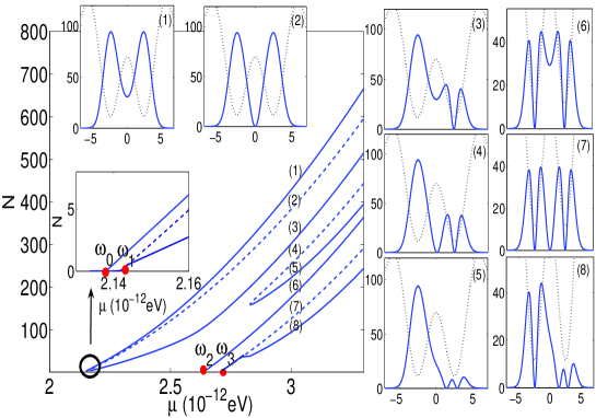
Figure 1: (Color online) Number of atoms as a function of the chemical potential for the different states. The potential parameters are $\Omega=0.1$, $k=\pi/5.37$ $\mu\text{m}^{-1}$ and $V_{0}=1.16\times 10^{-12}$ eV. The insets show the densities of the different states for $\mu=3\times 10^{-12}$ eV.

Fig. 1 shows the number of atoms as a function of the chemical potential for different branches of solutions. The insets show the spatial density profiles for $\mu=3\times 10^{-12}$ eV, with the units of the horizontal and vertical axes being given by $\mu m$ and $1/\mu m$, respectively.

Branch (1) corresponds to the states with the largest number of atoms, for fixed chemical potential. The respective states are symmetric and have no nodes. Continuation of this symmetric branch to the linear limit ends at the eigenvalue $\omega_{0}$, corresponding to the ground state of the linear problem.

The second branch [branch (2)] starts from the first excited state in the linear limit, $\mu\rightarrow\omega_{1}$ as $N\rightarrow 0$. The wavefunctions of the states of this branch are antisymmetric and have a node at the center of the barrier, while their densities are symmetric. From this density symmetric one-soliton branch, two asymmetric one-soliton branches, namely branch (3) and its mirror image with respect to the $z=0$ axis, bifurcate close to the linear limit, at $\mu\simeq 2.144\times 10^{-12}$ eV – see the close-up inset. Let us define a local occupation number, i.e., number of atoms in the different wells, as the integral over the density up to the center of the barrier (see also Sec. V below). The occupation number in the well with the node is then smaller than the occupation number without the node. This can be explained by the fact that the state with one node is the first excited state, characterized by a higher energy than the one without a node, which is the ground state. Thus, in order to balance the chemical potential in both wells one needs a larger interaction energy (i.e., more atoms) in the well without a node. Note that the macroscopic quantum self-trapping (MQST) state as predicted in Ref smerzi is not considered in what follows. The reason for that is that the MQST is a running phase state while our bifurcation analysis below focuses on the stationary states of the system. Branches (4) and (5) have no linear counterparts since at $\mu\simeq 2.828\times 10^{-12}$ eV they “collide” and disappear. The states that belong to these branches are asymmetric, exhibiting two nodes. The state with larger number of atoms (for a fixed chemical potential) has one node approximately at the barrier and one node in one well. The other state has both nodes in one well. Once again, the occupation number in the well with two nodes is less than the one of the well with one node, so as to balance the chemical potential.

Branch (6) starts from the second excited state of the linear problem, hence $\mu\rightarrow\omega_{2}$ as $N\rightarrow 0$. Therefore, the density of the respective state is symmetric and there is one node in each well.

Branch (7) starts from the third excited state of the linear problem, and $\mu\rightarrow\omega_{3}$ as $N\rightarrow 0$. The states belonging to this branch have three nodes, one located in each well and one at the barrier, and are symmetric. Close to the linear limit, at $\mu\simeq 2.795\times 10^{-12}$ eV, two asymmetric three-soliton branches, namely branch (8) and its mirror image with respect to the $z=0$ axis, bifurcate from this state. This state has two nodes in one well and one in the other. The occupation number in the well with more nodes is smaller than in the well with just one node in order to balance the chemical potential. Notice that there exist two more three-soliton branches without linear counterparts, but they only occur at higher chemical potentials — where the BEC has occupied four-wells rather than two — so they will not be considered here.

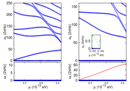
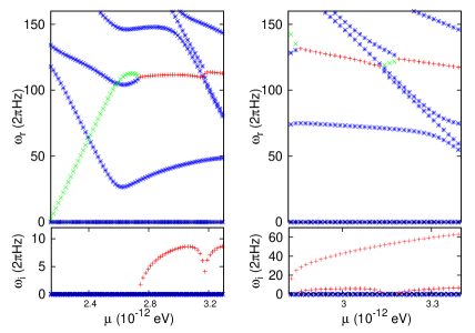
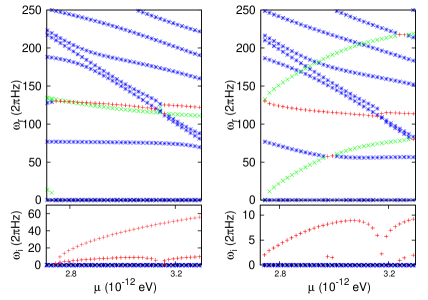
Figure 2: (Color online) BdG Spectrum of the states shown in Fig. 1. First panel shows the spectrum of the first branch, second panel the spectrum of the second branch and so forth. The (blue) $\divideontimes$ symbol denotes an eigenmode of positive Krein sign (or zero Krein sign for a vanishing eigenfrequency), the (green) $\times$ symbol an eigenmode of negative Krein sign, and the (red) $+$ symbol an eigenmode associated to a vanishing Krein sign with complex/imaginary eigenfrequency.

Next, let us study the stability of the states belonging to the above mentioned branches by considering the respective excitation spectra, shown in Fig. 2. In this figure, the (blue) $\divideontimes$ symbol denotes a positive Krein sign mode (or a zero one for a vanishing frequency), the (green) $\times$ symbol a negative Krein sign mode, i.e., a negative energy anomalous mode, and the (red) ($+$) symbol a vanishing Krein sign, i.e., an eigenmode associated with complex/imaginary eigenfrequency. Generally speaking, there are two different kinds of instability, corresponding to the cases of either a purely imaginary eigenfrequency, or a genuinely complex eigenfrequency. The latter case gives rise to the so-called oscillatory instability, stemming from the collision of a negative energy mode with one of positive energy.

The first panel of Fig. 2 shows the BdG spectra along the first branch. The imaginary part is zero for every value of the chemical potential, a fact reflecting the stability of this state. The absence of negative energy modes is expected, as this state is actually the ground state of the system. Since the BdG spectrum refers to all excitations of the state, one can attribute in the linear limit to each mode an excited state of the linear problem. The energy gap between the ground state and the first excited state corresponds to the energy of the first mode. Since the frequency of the so-called bosonic Josephson junction, namely the oscillation frequency characterizing the transfer of atoms between the two wells, is equal to this frequency in the linear limit, this mode is connected to the oscillation of atoms between the two wells. We investigate this fact in more detail below (see Sec. V) by direct simulations in the framework of Eq. (1). The frequency value of the second nonzero BdG mode of the ground state spectrum is correspondingly equal to the energy gap between the ground state and the second excited state in the linear limit, and so forth. We define the difference in the way that these frequency differences are positive.

The second panel shows the BdG spectra along the second branch, solutions of which represent states with a density minimum at the center of the barrier. In the linear limit one can assign to each mode an energy difference of the linear problem similar as in the BdG spectrum of the ground state. However in this case the frequency difference of the first excited state to the ground state is negative (according to our definition) leading to a negative energy mode. As one can see in the inset, the lowest mode has negative energy close to the linear limit. However, increasing the chemical potential the eigenfrequency of this mode is moving rapidly towards the origin of the spectrum and, at $\mu=2.1437\times 10^{-12}$ eV, becomes and remains purely imaginary, thus carrying zero energy (red $+$ symbols). This happens exactly at the point where the third branch bifurcates as one can see in the inset of Fig. 1. For the above mentioned potential parameters, this bifurcation happens in the weakly-interacting regime, where Eq. (3) reduces to the cubic NLS equation. Thus, one can apply the Galerkin-type approach of Ref. Theo06 and find that the critical value of the norm $N$ at which the bifurcation occurs is given by

$$N_{\text{cr}}=\frac{\omega_{1}-\omega_{0}}{3B-A_{1}},$$ (17)

where $\omega_{0,1}$ are the first two lowest eigenvalues of the operator $1+\hat{H}$, $A_{1}=\int{\psi_{1}^{4}dz}$, $B=\int{\psi_{0}^{2}\psi_{1}^{2}dz}$, while $\psi_{0,1}$ denote the ground state and the first excited state of the operator $1+\hat{H}$, respectively. One can also determine the critical chemical potential at which the symmetry breaking is expected to occur, namely $\mu_{cr}=1+\omega_{0}+3BN_{\text{cr}}$ Theo06 leading for (these parameter values) to $\mu_{\text{cr}}=2.1436\times 10^{-12}$ eV, which is in very good agreement with our numerical findings.

The third panel shows the BdG spectra along the third branch which bifurcates at $\mu=2.1437\times 10^{-12}$ eV from the second one. All the eigenfrequencies of the arising asymmetric state are real close to the linear limit, thus it is concluded that this state is linearly stable and that the bifurcation is a supercritical pitchfork. This state has one negative energy mode as well, since it is a one-soliton state. The eigenfrequency of the negative energy mode increases with increasing chemical potential, passes through the mode corresponding to the second excited state of the linear limiting case, and finally collides at some critical value of the chemical potential, $\mu=2.76\times 10^{-12}$ eV, with the mode corresponding to the third excited state; this results in the generation of a quartet of unstable eigenfrequencies and, at this point, the state becomes oscillatory unstable. However, the magnitude of the instability is much smaller than in the previous case of the purely imaginary eigenfrequency.

The fourth and fifth panel show the spectra along the fourth and fifth branch, the solutions of which correspond to asymmetric two-soliton states having no linear counter-part. The previous one has got one imaginary and one negative energy mode and the latter one has two negative energy modes. These modes result from the presence of two dark solitons. The state considered in the fourth panel has two dark solitons, one soliton located approximately at the barrier and one soliton in one well. The eigenfrequency corresponding to the former one is purely imaginary and looks similar to the mode of the symmetric one soliton state of the second panel. The eigenfrequency of the other anomalous mode decreases with increasing chemical potential and collides with a mode with positive energy, thus generating a quartet of complex eigenfrequencies. The magnitude of the imaginary part is again much smaller than the magnitude of the purely imaginary eigenfrequency. The generation of dynamic instabilities is illustrated e.g. in panel five. The collision of one of the anomalous modes with a mode of positive Krein sign could lead to the emergence of a quartet of complex eigenfrequencies, resulting in the concurrent presence of an apparent level crossing in the real part of the eigenfrequency along with a nonzero imaginary part of the relevant eigenfrequency mode.

At $\mu\simeq 2.828\times 10^{-12}$ eV, the states of the fourth and fifth branch collide and disappear as can be seen in Fig. 1. Just before the collision (for slightly larger $\mu$), the state of the fourth branch is unstable due to the presence of a mode with imaginary eigenfrequency in the BdG spectrum, while the state of the fifth branch is linearly stable since all the BdG eigenfrequencies have only real parts. Thus, it can be concluded that, at this critical point, a saddle-node bifurcation occurs, readily destroying these two states.

The sixth panel shows the BdG spectra along the sixth branch, the solutions of which correspond to symmetric two-soliton states. This branch has a linear counterpart, and we can assign to each mode in the linear limit an energy difference of the linear problem. The negative energy modes occur for negative energy differences, e.g., at the energy difference to the ground state and the first excited state. The anomalous modes here are close to being degenerate. Physically speaking, this reflects the fact that the dark solitons are essentially decoupled at the linear limit due to the presence of the optical lattice. The negative energy modes are not the modes with the lowest eigenfrequency. The energy gaps between the second excited state and the third and fourth excited state, respectively, are smaller than the gaps between the ground state and the first excited state. Therefore, these modes with positive energy occur in the linear limit at lower frequencies. One of the negative energy modes collides at some critical value of the chemical potential with the mode stemming from the fourth excited state and forms a quartet of complex frequencies, thus leading to an oscillatory instability.

The seventh panel shows the BdG spectra along the seventh branch, the solutions of which corresponds to the symmetric three-soliton state exhibiting a linear counterpart. The negative energy modes occur at the energy gaps to the ground state, the first and the second excited states. The eigenfrequency of the latter becomes, for increasing $\mu$, purely imaginary at the point where the eighth branch bifurcates. The other two anomalous modes are almost degenerate, reflecting again the fact that the solitons in the different wells are almost decoupled. One of the negative energy modes collides with a mode with positive energy and forms a quartet of complex frequencies. However, the magnitude of the imaginary part is much smaller than the magnitude of the purely imaginary mode. The behavior of the purely imaginary mode is similar to the behavior of the mode in panel two (describing a single soliton at the center of the barrier). The behavior of the other two modes is similar to the modes in panel six describing one soliton in each well.

Finally, the eighth panel shows the BdG spectra along the eighth branch, the solutions of which corresponds to the asymmetric three-soliton state. This state, which has two solitons in one well and one soliton in the other well, emerges at $\mu\sim 2.74\times 10^{-12}$ eV, where the seventh state (i.e., the one corresponding to the nonlinear continuation of the third excited state), becomes unstable. The critical value of the number of atoms for which the bifurcation occurs can be predicted in the same way as for the bifurcation of the one soliton branch; the result is:

$$N_{\text{cr}}^{(3)}=\frac{\omega_{3}-\omega_{2}}{3D-C_{1}},$$ (18)

where $\omega_{2,3}$ are the third and fourth lowest eigenvalues of operator $1+\hat{H}$, $C_{1}=\int{\psi_{3}^{4}dz}$, $B=\int{\psi_{2}^{2}\psi_{3}^{2}dz}$, while $\psi_{2,3}$ denote the second and third excited state of the operator $1+\hat{H}$, respectively. The corresponding critical chemical potential is then given by $\mu_{cr}^{(3)}=1+\omega_{2}+3BN_{\text{cr}}^{(3)}$ leading (for these parameters) to $\mu_{\text{cr}}^{(3)}=2.7420\times 10^{-12}$ eV, which is in very good agreement with the numerical critical point given above.

Right after the bifurcation, the asymmetric three soliton states are stable and, thus, we can conclude that the bifurcation is of the supercritical pitchfork type. Two modes look similar to the negative energy modes in panel five describing a two-soliton state in one well and the third mode looks similar to a mode of one-soliton in a harmonic trap.

From the above analysis, we can readily derive some general conclusions concerning dark soliton states in a double well potential. The sum of negative energy modes and imaginary eigenfrequency modes is equal to the number of nodes in the wavefunction profile which, for large values of the chemical potential, represent dark solitons. In the linear limit, the BdG eigenfrequencies of a state correspond to the energy differences between that and other states of the linear system. For a negative energy difference the corresponding mode has a negative energy. Dark solitons located at the center of the barrier are known to be linearly unstable (for sufficiently high chemical potential) associated with a purely imaginary eigenfrequency weol ; ichihara . Thus, symmetric states with an odd number of nodes always have a mode which, above a critical value of the chemical potential, becomes purely imaginary. At this critical point additional stable asymmetric dark-soliton states emerge through supercritical pitchfork bifurcations.

IV Statics vs. dynamics of dark soliton states

IV.1 The one-soliton state

Having investigated in detail the statics of matter-wave dark solitons in double-well potentials, we now proceed to compare these results to the soliton dynamics, using the theoretical background exposed in Sec. III.B. Particularly, considering the case of a single dark soliton, we can readily obtain from Eqs. (12) and (14) the following approximate equation of motion for the dark soliton center:

$$\frac{d^{2}z_{0}}{dt^{2}}=-\omega_{\rm ds}^{2}z_{0}+\frac{1}{2}kV_{0}\sin(2kz_{0}).$$ (19)

It is straightforward to find the fixed points $z_{\rm o},p_{\rm o}\equiv dz_{\rm o}/dt$ of the above dynamical system, which are given by

$$p_{\rm o}=0,\qquad z_{\rm o}=\frac{kV_{0}}{2\omega_{\rm ds}^{2}}\sin(2kz_{\rm o}).$$ (20)

It is clear that the fixed points correspond to intersections of the straight line $f_{1}(z_{\rm o})=z_{\rm o}$ and the sinusoidal curve $f_{2}(z_{\rm o})=\frac{kV_{0}}{2\omega_{ds}^{2}}\sin(2kz_{\rm o})$. The fixed point at $(z_{\rm o},p_{\rm o})=(0,0)$ exists for all choices of ($\Omega,V_{0},k$). This equilibrium corresponds to the symmetric one-soliton state, namely a stationary black soliton located at the center of the potential. In the absence of the optical lattice (i.e., for $V_{0}=0$) this is the only existing fixed point, i.e., in the case of a purely harmonic trap, only a symmetric one-soliton state can exist, which originates from the first excited state of the linear problem. On the other hand, when the optical lattice is present (i.e., for $V_{0}\neq 0$), this situation changes and more fixed points arise when the slope of the curve $f_{2}(z_{\rm o})$ at the origin becomes larger than the one of the straight line $f_{1}(z_{\rm o})$, namely when $k^{2}V_{0}/\omega_{\rm ds}^{2}>1$, two new fixed points appear through a supercritical pitchfork, with the newly emerging states corresponding to the bifurcating asymmetric one-soliton states. Therefore, the bifurcating state appears only for a sufficiently strong optical lattice, such that $V_{0}>V_{0,cr}\equiv\omega_{\rm ds}^{2}/k^{2}$. Note that for even larger values of the parameter $k^{2}V_{0}/\omega_{\rm ds}^{2}$ more fixed points appear, corresponding to solitons located in further (i.e., more remote from the trap center) wells of the optical lattice; for this reason, these states are not considered herein.

Let us now investigate the spectral stability of the fixed points employing the linearization technique (see, e.g., Ref. Strogatz ). Particularly, we first find the corresponding Jacobian matrix (evaluated at the fixed points), which is given by:

$${\bf J}=\left(\begin{array}[]{cc}0&1\\ -\omega_{\rm ds}^{2}+k^{2}V_{0}\cos(2kz_{0})&0\\ \end{array}\right).$$

When evaluated at the trivial fixed point $(z_{\rm o},p_{\rm o})=(0,0)$, the corresponding eigenvalue problem for the Jacobian, $\det({\bf J}-\lambda{\bf I})=0$, leads to eigenvalues $\lambda^{2}=-\omega_{\rm ds}^{2}+k^{2}V_{0}$. It is clear that in the case of $k^{2}V_{0}/\omega_{\rm ds}^{2}<1$, the eigenvalues are imaginary (note that, accordingly, the eigenfrequencies are real since $\omega=i\lambda$) and, thus, the fixed point $(0,0)$ is a center. In this case, if the dark soliton is weakly displaced from the center of the trap, it performs harmonic oscillations around the center with an oscillation frequency given by $\omega_{\rm osc}=\sqrt{\omega^{2}_{\rm ds}-k^{2}V_{0}}$. On the other hand, if $k^{2}\frac{V_{0}}{\omega_{\rm ds}^{2}}>1$ then the eigenvalues become real (and, accordingly, the eigenfrequencies are imaginary), hence $(0,0)$ becomes a saddle point, while the respective imaginary eigenfrequency is given by $\omega_{\rm osc}=i\sqrt{|\omega^{2}_{\rm ds}-k^{2}V_{0}|}$. For the newly bifurcating (stable, since $V_{0}>\omega_{\rm ds}^{2}/k^{2}$) fixed points one can obtain the following eigenfrequency

$$\omega_{\rm osc}=\sqrt{\omega_{ds}^{2}-k^{2}V_{0}\cos(2kz_{0})}.$$ (21)

From the above analysis it is clear that the supercritical pitchfork occurs at

$$V_{0,cr}=\frac{\omega_{\rm ds}^{2}}{k^{2}}.$$ (22)

Based on the above, one can make the following estimates and comparisons to numerical results: in the TF limit, and in the weakly-interacting case (i.e., in the framework of the 1D cubic GP equation), the dark soliton oscillation frequency is predicted to be $\omega_{z}/\sqrt{2}=28.28$Hz. However, as mentioned in Sec. III.B, a larger value of this frequency is expected in the framework of Eq. (1), due to the effect of the dimensionality of the system. Employing a BdG analysis in the case of a pure harmonic trap, we find that the anomalous mode eigenfrequency (i.e., the soliton oscillation frequency) decreases with increasing chemical potential and asymptotically reaches the value $\omega_{\text{ds}}=30.36$Hz (see first panel of Fig. 4 below). Using this value (and for $k=\pi/5.37\mu m^{-1}$), one obtains $V_{0,cr}=9.6\times 10^{-14}$ eV.

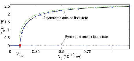
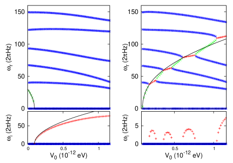
Figure 3: (Color online) Top panel: Fixed points (lines) of the dynamical system (19) and position of the soliton (open circles) calculated by the Eq. (1) with $\mu=3.8\times 10^{-12}$ eV. Bottom left (right) panel: BdG spectra of the symmetric (asymmetric) one-soliton state for $\mu=3.8\times 10^{-12}$ eV as a function of $V_{0}$.

In the top panel of Fig. 3, we show the fixed points of the dynamical system (19) as a function of the optical lattice strength $V_{0}$. The dash-dotted (green) line denotes the non-zero fixed point calculated from Eq. (20) with $\omega_{\rm ds}=\omega_{z}/\sqrt{2}$, while the solid (black) line denotes the non-zero fixed point calculated from Eq. (20) with $\omega_{\text{\rm ds}}=30.36$ Hz. Furthermore, the circles denote the position of the node of the nonlinear stationary state — i.e., the position of the dark soliton — obtained by numerical integration of Eq. (1) with $\mu=3.8\times 10^{-12}$ eV (in the TF limit). Clearly, at $V_{0,cr}\simeq 9.6\times 10^{-14}$ eV, the asymmetric one-soliton branch bifurcates through a supercritical pitchfork bifurcation; notice the excellent agreement between the two approaches.

The bottom left and right panels of Fig. 3 show the BdG spectra of the symmetric and asymmetric one soliton state, respectively, as a function of the optical lattice strength (for a fixed chemical potential, $\mu=3.8\times 10^{-12}$ eV). For sufficiently small lattice strength, $V_{0}<V_{0,cr}$, the symmetric state is stable, while when the lattice strength $V_{0}$ is increased, the magnitude of the instability grows and the prediction of Eq. (21) deviates from the results obtained from the integration of Eq. (3). To explain this discrepancy, it is relevant to recall that the result of the perturbation theory of Sec. II.B is valid only if all perturbation terms are small and of the same order. Nevertheless, for the symmetric one soliton state — with the soliton located at zero — the magnitude of the perturbation term corresponding to the harmonic trap (optical lattice) has its smallest (largest) value; thus, for large $V_{0}$, these perturbations cannot be of the same order. As concerns the asymmetric state, the prediction of Eq. (21) is in fairly good agreement to the results obtained from the numerical integration of Eq. (3). However, Eq. (21) cannot predict oscillatory instabilities (associated with the existence of complex eigenfrequencies), which occur when the anomalous mode collides with a mode of the background condensate. This can readily be understood by the fact that the derivation of the equation of motion of the dark soliton relies on the assumption that the soliton is decoupled from the background (see, e.g., Refs. motion2 and revnonlin for details), which is not the case for oscillatory instabilities.

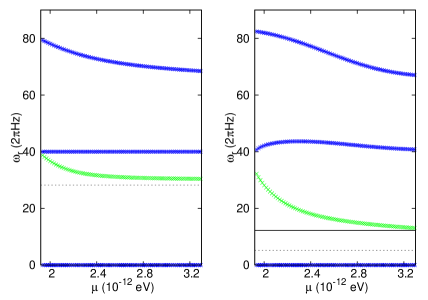
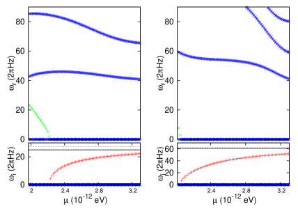
Figure 4: (Color online) BdG spectra for four different values of the optical lattice strength for the symmetric dark soliton state (with the soliton located at the trap center): from left to right, $V_{0}=0$, $V_{0}=8.3\times 10^{-14}$ eV, $V_{0}=1.65\times 10^{-13}$ eV and $V_{0}=4.96\times 10^{-13}$ eV. The solid lines correspond to the predictions of Eq. (21). Symbol $\divideontimes$ (blue) denotes a positive (or zero for a vanishing eigenfrequency), symbol $\times$ (green) a negative and symbol $+$ (red) a vanishing Krein sign mode (for non-zero eigenfrequencies).

Next, let us study the continuation of both symmetric and asymmetric one-soliton states with increasing chemical potential for various values of the optical lattice strength.

First, we consider the symmetric one-soliton state and in Fig. 4 we show the BdG spectra along the corresponding branch. The first panel shows the case of a pure harmonic trap, i.e., $V_{0}=0$, and the dashed line is the prediction from Eq. (21) using $\omega_{\rm ds}=\omega_{z}/\sqrt{2}$. It is clear that the eigenfrequencies are real, indicating the stability of this state for all values of the chemical potential. The figure shows the constant eigenfrequency of the dipolar mode [see straight (blue) line] at the value of the trap frequency $\omega_{z}$ and the anomalous mode bifurcating from the dipolar mode in the linear limit. As mentioned above, the eigenfrequency of the anomalous mode reaches asymptotically the value $\omega_{\text{ds}}=30.36$ Hz.

The second panel of Fig. 4 shows the BdG spectrum for $V_{0}=8.3\times 10^{-14}$ eV. All eigenfrequencies are real, so the state is still stable. The dashed line is the prediction by Eq. (21) using $\omega_{ds}=\omega_{z}/\sqrt{2}$, while the solid line is the prediction with $\omega_{\text{ds}}=30.36$ Hz. The dipole mode remains approximately constant for such a small optical lattice strength. However, the degeneracy of the anomalous mode and the dipole mode in the linear limit disappears.

The third panel shows the spectra for $V_{0}=1.65\times 10^{-13}$ eV. In this case, the anomalous mode becomes purely imaginary for increasing chemical potential, reflecting the fact that the state becomes unstable. Notice that the numerical result and the analytical prediction, $\omega_{ODE}=i\sqrt{|\omega^{2}_{\rm ds}-k^{2}V_{0}|}$, are in a good agreement for large values of the chemical potential, where the TF limit is reached and Eq. (19) is valid. Since $V_{0}>{V}_{0,cr}$, this state is expected to be unstable in the TF limit.

The fourth panel shows the spectra for $V_{0}=4.96\times 10^{-13}$ eV. In this case, the anomalous mode becomes purely imaginary already at small chemical potentials. Furthermore, the dipole mode eigenfrequency is now significantly modified, upon the reported interval of changes of the chemical potential. The analytical prediction agrees again well with the numerical BdG result in the TF limit.

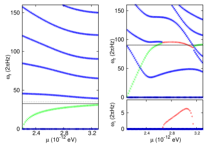
Figure 5: (Color online) BdG spectra for $V_{0}=1.65\times 10^{-13}$ eV (left panel) and $V_{0}=8.3\times 10^{-13}$ eV (right panel) for the asymmetric dark soliton state, bifurcating from the symmetric one. The notation of eigenstates is the same as in Fig. 4.

Next, we consider the continuation with increasing chemical potential of the asymmetric states bifurcating from the symmetric one when the latter becomes unstable. Fig. 5 shows the BdG spectra along the asymmetric one-soliton state for $V_{0}=1.65\times 10^{-13}$ eV and $V_{0}=8.3\times 10^{-13}$ eV. The analytical predictions of Eq. (21) with $\omega_{\rm ds}=\omega_{z}/\sqrt{2}$ and $\omega_{\text{ds}}=30.36$Hz, respectively plotted with dashed and solid lines are in good agreement with the respective anomalous mode eigenfrequencies. In the case of $V_{0}=8.3\times 10^{-13}$ eV, the difference between the result of Eq. (21) using $\omega_{ds}=\omega_{z}/\sqrt{2}$ and $\omega_{\text{ds}}=30.36$ Hz is small, showing that the dynamics is mostly governed by the potential term stemming from the optical lattice.

IV.2 Two dark-soliton states

We now consider the case of the two-soliton state, for which we need to incorporate the interaction potential in order to describe their dynamics. Particularly, according to the theoretical framework of Sec. II.B, the effective potential describing the dynamics of two solitons located at $z_{1}$ and $z_{2}$ has the following form:

$$V_{\text{eff}}(z_{1},z_{2})=\omega_{\rm ds}^{2}(z_{1}^{2}+z_{2}^{2})+\frac{V_{0}}{2}(\cos(2kz_{1})+\cos(2kz_{2}))+\frac{2n_{0}}{\sinh^{2}(\sqrt{n_{0}}(z_{2}-z_{1}))}.$$ (23)

Using $d^{2}z_{i}/dt^{2}=-(1/2)dV_{\text{eff}}(z_{1},z_{2})/dz_{i}$ (with $i=1,2$) as per Eq. (12), it is straightforward to derive the following system of equations of motion,

$$\frac{d^{2}z_{1}}{dt^{2}} = -\omega_{\rm ds}^{2}z_{1}+\frac{1}{2}kV_{0}\sin(2kz_{1})-2n_{0}^{3/2}\coth(\sqrt{n_{0}}(z_{2}-z_{1})){\rm csch}^{2}(\sqrt{n_{0}}(z_{2}-z_{1})),$$ (24)

$$\frac{d^{2}z_{2}}{dt^{2}} = -\omega_{\rm ds}^{2}z_{2}+\frac{1}{2}kV_{0}\sin(2kz_{2})+2n_{0}^{3/2}\coth(\sqrt{n_{0}}(z_{2}-z_{1})){\rm csch}^{2}(\sqrt{n_{0}}(z_{2}-z_{1})),$$ (25)

which, accordingly, leads to the following system for the fixed points ($z^{(1)}_{\rm o}$, $z^{(2)}_{\rm o}$):

$$z^{(1)}_{\rm o} = \frac{V_{0}k}{2\omega_{\rm ds}^{2}}\sin(2kz^{(1)}_{\rm o})-\frac{n_{0}^{3/2}}{\omega_{\rm ds}^{2}}\coth(\sqrt{n_{0}}(z^{(2)}_{\rm o}-z^{(1)}_{\rm o})){\rm csch}^{2}(\sqrt{n_{0}}(z^{(2)}_{\rm o}-z^{(1)}_{\rm o})),$$ (26)

$$z^{(2)}_{\rm o} = \frac{V_{0}k}{2\omega_{\rm ds}^{2}}\sin(2kz^{(2)}_{\rm o})+\frac{n_{0}^{3/2}}{\omega_{\rm ds}^{2}}\coth(\sqrt{n_{0}}(z^{(2)}_{\rm o}-z^{(1)}_{\rm o})){\rm csch}^{2}(\sqrt{n_{0}}(z^{(2)}_{\rm o}-z^{(1)}_{\rm o})).$$ (27)

Thus, the fixed points for the two soliton states depend on the density of the background cloud and thereby on the chemical potential. Due to the presence of the external potentials, the density of the background is inhomogeneous. In our analysis, we replace the inhomogeneous density, with the density of the background at $z=0$ using the TF approximation; namely, $n_{0}\rightarrow n_{0}(z=0)=((\mu-V_{0})^{2}-1)/4$.

Considering small deviations from the fixed points, i.e., $z_{i}=z^{(i)}_{\rm o}+\epsilon\eta_{i}\exp(i\omega t)$ (with $i=1,2$), leads to the eigenvalue problem for the normal modes:

$$\omega^{2}\mathbf{\eta}=\left(\begin{array}[]{cc}A(z^{(1)}_{\rm o})+B(z^{(1)}_{\rm o},z^{(2)}_{\rm o})&-B(z^{(1)}_{\rm o},z^{(2)}_{\rm o})\\ -B(z^{(1)}_{\rm o},z^{(2)}_{\rm o})&A(z^{(2)}_{\rm o})+B(z^{(2)}_{\rm o},z^{(1)}_{\rm o})\\ \end{array}\right)\mathbf{\eta}$$ (28)

with

$$A(x) = \omega_{\rm ds}^{2}-V_{0}k^{2}\cos(2kx)$$ (29)

$$B(x,y) = 4n_{0}^{2}\coth^{2}(\sqrt{n_{0}}(x-y)){\rm csch}^{2}(\sqrt{n_{0}}(x-y))+2n_{0}^{2}{\rm csch}^{4}(\sqrt{n_{0}}(x-y)).$$ (30)

Diagonalizing the above matrix, we obtain the eigenfrequencies of the two anomalous modes of the two-soliton states. Notice that since different two soliton states lead to different fixed points, the oscillation frequencies for the two solitons will differ as well. Negative eigenvalues of this $2\times 2$ system lead to imaginary frequencies describing unstable states; however, as mentioned in the previous section, one cannot describe oscillatory instabilities.

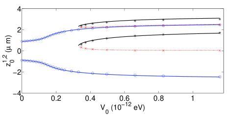
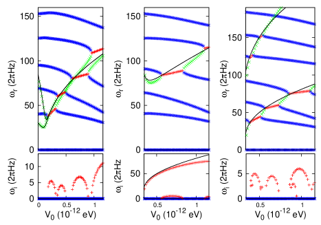
Figure 6: (Color online) Top panels: Fixed points (lines) of the system (26)-(27) and position of the solitons (circles for the symmetric two-soliton state, $\times$ for the two-soliton branch with one soliton near the center and one in one well, and stars for the state with both dark solitons in the same well) calculated by the numerical integration of Eq. (1) for $\mu=3.8\times 10^{-12}$ eV. Bottom panels: BdG spectra of the two-soliton states for $\mu=3.8\times 10^{-12}$ eV as a function of $V_{0}$; left corresponds to the symmetric two-soliton state, middle to the always unstable state with one soliton near the center and one in one well, while the right corresponds to the state with both dark solitons in the same well. Notice also the agreement of the theoretically predicted modes from Eq. (28) with the numerical ones.

In the top panel of Fig. 6, we show the fixed points of the system (26)-(27) and the zero points of the solutions with two nodes of Eq. (1) corresponding to the positions of the two solitons as a function of $V_{0}$ (the chemical potential is fixed: $\mu=3.6\times 10^{-13}$ eV). For small $V_{0}$ there exists only the symmetric solution with two nodes. However, for $V_{0,cr}=3.4\times 10^{-12}$ eV, two asymmetric states appear stemming from a saddle-node bifurcation. For all three states, the agreement between the fixed points obtained from Eqs. (26)-(27) and the position of the solitons is excellent.

The bottom panels of Fig. 6 show the BdG spectra for the symmetric and the two asymmetric two soliton states as a function of $V_{0}$ for fixed $\mu=3.8\times 10^{-12}$ eV. The solid lines correspond to the normal modes of Eqs. (24)-(25) around the corresponding fixed points. For a small optical lattice strength $V_{0}$, the two anomalous modes of the symmetric states have a different magnitude, which indicates that the solitons are coupled. However, for increasing $V_{0}$, this difference decreases and, thus, the coupling between the soliton becomes weaker. Notice that for an optical lattice strength $V_{0}\simeq 3.6\times 10^{-12}$ the two modes become of the same order, a fact that indicates that the two solitons become eventually decoupled. The prediction of Eqs. (24)-(25) agrees very well with the numerical results obtained via the BdG analysis for the anomalous modes. The second panel shows the BdG spectrum of the asymmetric state with one soliton located approximately at the center of the barrier. The latter, leads to a purely imaginary mode with an increasing magnitude with increasing $V_{0}$. The increase of the magnitude of this mode results from the increase of the height of the barrier. For large $V_{0}$ the prediction of Eqs. (24)-(25) deviates from the result obtained in the framework of Eq. (1): the contributions of the perturbation terms are not of the same order and, thus, perturbation theory fails in this case. The third panel shows the BdG spectrum for the second asymmetric state with two solitons in one well. The difference between the modes is always large, a fact indicating the strong coupling between the two solitons. With increasing lattice strength $V_{0}$, the eigenfrequencies of the anomalous modes increases too. The predictions of Eqs. (24)-(25) agree once again well with the BdG results; nevertheless, as in previous cases, Eqs. (24)-(25) cannot predict oscillatory instabilities.

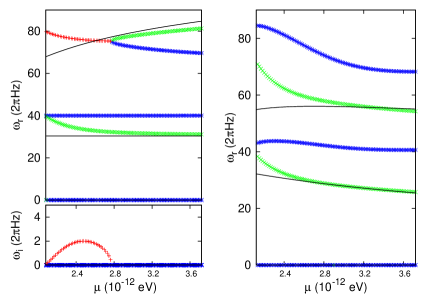
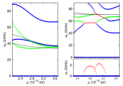
Figure 7: (Color online) BdG spectra for different values of the optical lattice strength; from left to right, $V_{0}=0$, $V_{0}=8.3\times 10^{-14}$ eV, $V_{0}=1.65\times 10^{-13}$ eV and $V_{0}=4.96\times 10^{-13}$ eV. The solid lines are the predictions of Eqs. (24)-(25) with a numerically determined oscillation frequency ($\omega_{\rm ds}$).

Next, let us consider a continuation with respect to the chemical potential. Fig. 7 shows the BdG spectra, and the predicted oscillation frequencies, for the symmetric two soliton state for different values of the optical lattice strength: $V_{0}=0$, $V_{0}=8.3\times 10^{-14}$ eV, $V_{0}=1.65\times 10^{-13}$ eV and $V_{0}=4.96\times 10^{-13}$ eV. In the case of a purely harmonic potential, $V_{0}=0$, one observes the constant eigenfrequency of the dipolar mode at $\omega_{z}$, as well as the eigenfrequency of one anomalous mode bifurcating from the dipolar mode in the linear limit. The eigenfrequency at $2\omega_{z}$ is imaginary due to a degeneracy of a negative and a positive Krein sign mode. The former one corresponds to the second anomalous mode and the latter one to the quadrupole mode. This degeneracy is lifted for increasing chemical potential. The predictions of Eqs. (24)-(25) agree very well with the BdG results for the anomalous modes in the case of large chemical potentials.

For $V_{0}=8.3\times 10^{-14}$ eV the degeneracy between the anomalous modes and the dipolar and the quadrupole mode is lifted in the linear limit. Thus, there exists an energy gap between the anomalous mode and the dipolar mode and, more importantly, an energy gap between the second anomalous mode and the quadrupole mode. A particularly useful conclusion stemming from the above findings is that the two soliton state can be stabilized in a harmonic trap by adding a small optical lattice.

For $V_{0}=1.65\times 10^{-13}$ eV the system is stable as well. The anomalous modes decrease with increasing chemical potential and reach similar values for a large chemical potential. This denotes that the two solitons are decoupled for a large chemical potential. This can be understood at least in the framework of the effective potential (23): the range of the interaction potential scales with the density $n_{0}$ of the background atom cloud and thereby with the chemical potential as well. Thus, for a large chemical potential, i.e., a large density, the interaction between solitons is strong but of short range too.

For $V_{0}=4.96\times 10^{-13}$ eV the anomalous modes have similar values even in the linear limit. Thus, the two solitons are already almost decoupled in the linear limit due to their large separation. The two anomalous modes collide with the dipolar and quadrupole modes for increasing chemical potential, leading to oscillatory instabilities, and bifurcate from these modes again for a larger chemical potential. Although the predictions of Eqs. (24)-(25) agree qualitatively with the BdG results, there is no quantitative agreement due to the crossings and collisions of the soliton modes with the modes of the condensate.

V Dark soliton dynamics: numerical results

So far, we have examined the existence, stability and bifurcations of the branches of dark-solitonic states in the double-well potential setting. We now proceed to investigate the dynamics of these states by direct numerical integration of Eq. (1), using as initial conditions stationary soliton states, perturbed along the direction of eigenvectors associated with particular eigenfrequencies (especially ones associated with instabilities). To better explain the above, we should recall that anomalous modes are connected to the positions and oscillation frequencies of the solitons; therefore, perturbations of stationary dark soliton states along the directions of the eigenvectors of the anomalous modes result in the displacement of the positions of the solitons, thus giving rise to interesting soliton dynamics.

Before proceeding with the dynamics of the (excited) soliton states, let us make a remark concerning the ground state of the system. As mentioned above, the value of the lowest BdG mode of the ground state is given, in the linear limit, by the energy difference between the ground state and the first excited state. However, this energy gap determines the oscillation frequency of atoms between the wells of the double-well potential, which suggests that the lowest BdG mode is connected to an oscillation between the wells. Let us define the atom numbers $N_{\rm L}$ and $N_{\rm R}$ in the left and right well, respectively, as $N_{\rm L}=\int_{-\infty}^{0}|\psi|^{2}dz$ and $N_{\rm R}=\int_{0}^{+\infty}|\psi|^{2}dz$ (the total number of atoms is $N=N_{\text{L}}+N_{\text{R}}$). In Fig 8, we show the time evolution of $N_{\text{L}}$ (solid line) and $N_{\text{R}}$ (dashed line) for the ground state, when perturbed by the eigenvector corresponding to the lowest BdG mode (parameter values are $\mu=3\times 10^{-12}$ eV and $V_{0}=1.12\times 10^{-12}$ eV). One can clearly observe the oscillation of the atom numbers in the different wells, with a characteristic frequency known as Josephson oscillation frequency smerzi , determined by the magnitude of the respective BdG eigenmode.

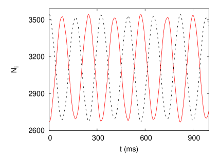
Figure 8: (Color online) Time evolution of the number of atoms $N_{\text{L}}$ (solid line) and $N_{\text{R}}$ (dashed line) in the left and right well of the double-well potential, respectively, for the ground state of the system perturbed by the lowest BdG mode. Parameter values are $\mu=3\times 10^{-12}$ eV and $V_{0}=1.12\times 10^{-12}$ eV.

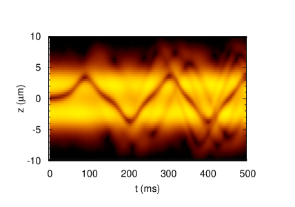
Figure 9: (Color online) Contour plot showing the space-time evolution of the density of the condensate, which carries the symmetric one-soliton state; dark corresponds to minimal and white to maximal density. The soliton is unstable and departs from the trap center after a short time period, performing subsequently large amplitude oscillations. Parameter values are $\mu=3\times 10^{-12}$ eV and $V_{0}=4.96\times 10^{-13}$.

Let us now proceed with the one-soliton states. Fig. 9 shows the time evolution of the symmetric one soliton state perturbed by the eigenvector corresponding to the unstable mode, for $\mu=3\times 10^{-12}$ eV and $V_{0}=4.96\times 10^{-13}$ eV. The instability manifests itself as a drift of the soliton from the trap center to the rims of the background atom cloud, where the soliton is reflected back and forth. One clearly observes that the soliton is located at an unstable position, since a small perturbation leads to a large amplitude oscillation of the soliton.

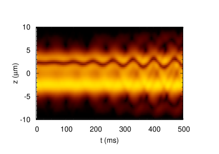
Figure 10: (Color online) Same as in Fig. 9, but for the asymmetric one-soliton state, for $\mu=3\times 10^{-12}$ eV for $V_{0}=8.27\times 10^{-13}$ eV.

On the other hand, Fig. 10 shows the time evolution of the asymmetric one soliton state perturbed by the eigenvector corresponding to the unstable mode for $\mu=3\times 10^{-12}$ eV for $V_{0}=8.27\times 10^{-13}$ eV. The corresponding state is subject to an oscillatory instability, which results in a growing amplitude of the soliton oscillation. However, in comparison to the previous case, the magnitude of the instability is much smaller and, thus, the increase of the amplitude is smaller (for the same time scale) as well.

Next, we consider the multi-soliton states and start with the symmetric two-soliton state which, for $\mu=3.3\times 10^{-12}$ eV and $V_{0}=8.27\times 10^{-14}$ eV, is found to be linearly stable. Numerical simulations, using as initial conditions this state perturbed by the eigenvectors corresponding to both anomalous modes, reveal that the two solitons perform oscillations with a constant amplitude and different frequencies. Specifically, the mode with smaller amplitude performs an in-phase oscillation (with the two solitons moving towards the same direction), whereas the mode with larger amplitude performs an out-of-phase oscillation (with the two solitons moving towards opposite directions) with a larger oscillation frequency. The existence of two different oscillation frequencies indicates the coupling of the dark solitons. This situation changes for a large optical lattice strength (e.g., $V_{0}=1.65\times 10^{-13}$ eV): in this case, the two dark solitons are decoupled, since the numerical simulations show that both the in-phase and out-of phase oscillations are characterized by almost the same frequency.

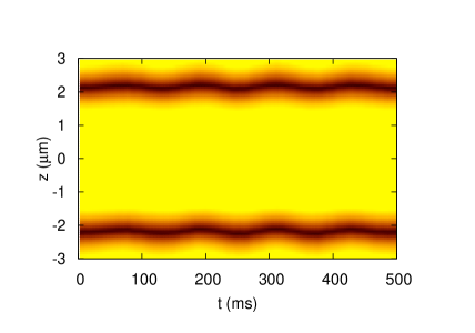
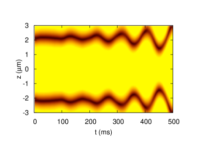
Figure 11: (Color online) Same as in Fig. 9, but for the symmetric two-soliton state with in-phase (left) anomalous mode and out-of-phase (right) imaginary mode perturbations, for $\mu=3.1\times 10^{-12}$ eV and $V_{0}=4.96\times 10^{-13}$ eV. The former anomalous eigenmode is stable, while the latter is unstable (as concluded also from the BdG analysis).

Fig. 11 shows the time evolution of the symmetric two-soliton state for $\mu=3.1\times 10^{-12}$ eV and $V_{0}=4.96\times 10^{-13}$ eV perturbed by the eigenvector corresponding to the anomalous mode associated with in-phase (left panel) and by the eigenvector corresponding to the imaginary mode out-of-phase (right panel) oscillations of the dark solitons. For these parameters, the BdG analysis predicts that the former mode is stable while the latter is unstable. This is confirmed by the direct simulations: it is clearly observed that the amplitude of the out-of-phase oscillation increases whereas the amplitude of the in-phase oscillation remains constant.

Figure 12: (Color online) Same as in Fig. 11, but for the symmetric two-soliton state, for $\mu=2.8\times 10^{-12}$ eV and $V_{0}=4.96\times 10^{-13}$ eV. Notice the reversal of stability of the two anomalous modes with respect to Fig. 11.

Finally, in Fig. 12 we show the time evolution of the symmetric two soliton state for $\mu=2.8\times 10^{-12}$ eV and $V_{0}=4.96\times 10^{-13}$ perturbed by the eigenvector corresponding to the anomalous mode with in-phase (left panel) and by the eigenvector corresponding to the imaginary mode out-of-phase (right panel) oscillations. For these parameters, the simulations show that the out-of-phase oscillation of the solitons is stable and the in-phase oscillation unstable, in agreement with the predictions of the BdG analysis.

VI Conclusions

In this work, we have performed a detailed study of the statics and dynamics of matter-wave dark solitons in a cigar-shaped Bose-Einstein condensate (BEC) confined in a double-well potential. The latter, was assumed to be formed as a combination of a usual harmonic trap and a periodic (optical lattice) potential. For our analysis, we have adopted and used an effectively 1D mean-field model, namely a Gross-Pitaevskii (GP)-like equation with a non-cubic nonlinearity, which has been used successfully in other works to describe dark solitons in BECs in the dimensionality crossover regime between 1D and 3D.

As a first step in our analysis, we studied the existence and stability of both the one- and multiple-dark soliton states. In particular, starting from the respective linear problem, we have used the continuation with respect to the chemical potential (number of atoms) to reveal the different branches of purely nonlinear solutions, including the ground state, as well as excited states, in the form of single or multiple dark solitons. We have shown that the presence of the optical lattice is crucial for the existence of nonlinear states that do not have a linear counterpart: these are actually asymmetric dark soliton states, with solitons located in one well (rather than in both wells) of the double-well potential, and do not exist in the non-interacting — linear — limit. We have systematically studied the bifurcations of the various branches of solutions and showed how each particular state emerges or disappears for certain chemical potential thresholds; the latter were determined analytically, in some cases, by using a Galerkin-type approach, in very good agreement with the numerical results. For each branch, we have also studied the stability of the pertinent solutions via a Bogoliubov-de Gennes (BdG) analysis. This way, we have discussed the role of the anomalous (negative energy) modes in the excitation spectra and revealed two types of instabilities of dark solitons, corresponding to either purely imaginary or genuinely complex eigenfrequencies; the latter were found to occur due to the collision of an anomalous mode with a positive energy mode and are associated with the so-called oscillatory instabilities of dark solitons.

We have also adopted a simple analytical model to study small-amplitude oscillations of the one- and multiple-dark-soliton states. Particularly, equations of motion for the single and multiple solitons were presented in the weakly-interacting limit (where the model becomes the usual cubic 1D GP equation), and modified them to take into regard the dimensionality of the system (i.e., the effect of transverse directions). The analysis of these equations of motion led to the determination of the characteristic soliton frequencies, which were then compared to the eigenfrequencies found in the framework of the BdG analysis; the agreement between the two was generally found to be very good. Perhaps even more importantly, the simple physical (i.e., particle) picture we adopted allowed us to reveal the role of the optical lattice strength (i.e., the height of the barrier in the double-well setting) in the stability of the dark solitons, as well as its role on the coupling between solitons. Particularly, it was found that sufficiently strong barriers lead to instability of symmetric and asymmetric soliton states, while it results in an effective decoupling of multi-solitons: the coupling between neighboring solitons as described by an effective repulsive potential, becomes negligible for sufficiently strong barriers. We should also note that generally the states possessing a dark soliton at the center of the trap were found to be most strongly unstable, due to the emergence of a progressively larger (the larger the nonlinearity) imaginary eigenfrequency.

Finally, we have performed systematic numerical simulations, based on direct numerical integration of the quasi-one-dimensional model, to investigate the dynamics of dark solitons in the double-well setup. We studied the manifestation of instabilities, when present, and found in all cases, a very good agreement between the predictions based on the BdG analysis and the numerical results. Instabilities have been observed to manifest themselves through the exponential divergence of the soliton from its initial location (when associated with an imaginary pair of eigenfrequencies) or the oscillatory growth (when associated with a complex quartet of eigenfrequencies).

An interesting direction for a future study would be a similar analysis in a higher-dimensional setting: this would refer to vortices confined in double-well potentials (or more complex “energy surfaces” such as quadruple-well potentials chenyu2d ) in higher-dimensional BECs. Such studies are presently in progress.

References

- (1) L. Pitaevskii and S. Stringari, Bose-Einstein Condensation (Oxford University Press, Oxford, 2003).
- (2) C. J. Pethick and H. Smith, Bose-Einstein Condensation in Dilute Gases (Cambridge University Press, Cambridge, 2001).
- (3) R. Carretero-González, D. J. Frantzeskakis, and P. G. Kevrekidis, Nonlinearity 21, R139 (2008).
- (4) P. G. Kevrekidis, D. J. Frantzeskakis, and R. Carretero-González (eds), Emergent Nonlinear Phenomena in Bose-Einstein Condensates: Theory and Experiment (Springer, Heidelberg, 2007).
- (5) S. Burger, K. Bongs, S. Dettmer, W. Ertmer, K. Sengstock, A. Sanpera, G. V. Shlyapnikov, and M. Lewenstein, Phys. Rev. Lett. 83, 5198 (1999).
- (6) J. Denschlag, J. E. Simsarian, D. L. Feder, C. W. Clark, L. A. Collins, J. Cubizolles, L. Deng, E. W. Hagley, K. Helmerson, W. P. Reinhardt, S. L. Rolston, B. I. Schneider, and W. D. Phillips, Science 287, 97 (2000).
- (7) Z. Dutton, M. Budde, C. Slowe, and L. V. Hau, Science 293, 663 (2001).
- (8) B. P. Anderson, P. C. Haljan, C. A. Regal, D. L. Feder, L. A. Collins, C. W. Clark, and E. A. Cornell, Phys. Rev. Lett. 86, 2926 (2001).
- (9) N. S. Ginsberg, J. Brand, and L. V. Hau, Phys. Rev. Lett. 94, 040403 (2005).
- (10) P. Engels and C. Atherton, Phys. Rev. Lett. 99, 160405 (2007).
- (11) C. Becker, S. Stellmer, P. Soltan-Panahi, S. Dörscher, M. Baumert, E.-M. Richter, J. Kronjäger, K. Bongs, and K. Sengstock, Nature Phys. 4, 496 (2008).
- (12) S. Stellmer, C. Becker, P. Soltan-Panahi, E.-M. Richter, S. Dörscher, M. Baumert, J. Kronjäger, K. Bongs, and K. Sengstock, Phys. Rev. Lett. 101, 120406 (2008).
- (13) A. Weller, J. P. Ronzheimer, C. Gross, J. Esteve, M. K. Oberthaler, D. J. Frantzeskakis, G. Theocharis, and P. G. Kevrekidis, Phys. Rev. Lett. 101, 130401 (2008).
- (14) I. Shomroni, E. Lahoud, S. Levy, and J. Steinhauer, Nature Phys. 5, 193 (2008).
- (15) G. Theocharis, A. Weller, J. P. Ronzheimer, C. Gross, M. K. Oberthaler, P. G. Kevrekidis, and D. J. Frantzeskakis, arXiv:0909.2122
- (16) W. H. Zurek, Phys. Rev. Lett. 102, 105702 (2009).
- (17) B. Damski and W. H. Zurek, arXiv:0909.0761.
- (18) J. Anglin, Nature Phys. 4, 437 (2008).
- (19) A. Negretti and C. Henkel, J. Phys. B: At. Mol. Opt. Phys. 37, L385 (2004).
- (20) A. Negretti, C. Henkel, and K. Mølmer, Phys. Rev. A 78, 023630 (2008).
- (21) P. O. Fedichev, A. E. Muryshev, and G. V. Shlyapnikov, Phys. Rev. A 60, 3220 (1999).
- (22) D. L. Feder, M. S. Pindzola, L. A. Collins, B. I. Schneider, and C. W. Clark, Phys. Rev. A 62, 053606 (2000).
- (23) A. E. Muryshev, G. V. Shlyapnikov, W. Ertmer, K. Sengstock, and M. Lewenstein, Phys. Rev. Lett. 89, 110401 (2002).
- (24) Th. Busch and J. R. Anglin, Phys. Rev. Lett. 84, 2298 (2000).
- (25) D. J. Frantzeskakis, G. Theocharis, F. K. Diakonos, P. Schmelcher, and Yu. S. Kivshar, Phys. Rev. A 66, 053608 (2002).
- (26) V. V. Konotop and L. Pitaevskii, Phys. Rev. Lett. 93, 240403 (2004).
- (27) G. Theocharis, P. Schmelcher, M. K. Oberthaler, P. G. Kevrekidis, and D. J. Frantzeskakis, Phys. Rev. A 72, 023609 (2005).
- (28) D. E. Pelinovsky, D. J. Frantzeskakis, and P. G. Kevrekidis, Phys. Rev. E 72, 016615 (2005).
- (29) V. A. Brazhnyi, V. V. Konotop, and L. P. Pitaevskii, Phys. Rev. A 73, 053601 (2006).
- (30) M. Coles, D.E. Pelinovsky, P.G. Kevrekidis, arXiv:0910.5249.
- (31) N. G. Parker, N. P. Proukakis, M. Leadbeater, and C. S. Adams, Phys. Rev. Lett. 90, 220401 (2003).
- (32) F. Kh. Abdullaev, B. B. Baizakov, S. A. Darmanyan, V. V. Konotop, and M. Salerno, Phys. Rev. A 64, 043606 (2001).
- (33) A. V. Yulin and D. V. Skryabin, Phys. Rev. A 67, 023611 (2003).
- (34) G. L. Alfimov, V. V. Konotop, and M. Salerno, Europhys. Lett. 58, 7 (2002).
- (35) V. V. Konotop and M. Salerno, Phys. Rev. A 65, 021602(R) (2002)
- (36) P. J. Y. Louis, E. A. Ostrovskaya, and Yu. S. Kivshar, J. Opt. B: Quantum Semiclass. Opt. 6, S309 (2004).
- (37) P. G. Kevrekidis, R. Carretero-González, G. Theocharis, D. J. Frantzeskakis, and B. A. Malomed, Phys. Rev. A 68, 035602 (2003) [see also Erratum: Phys. Rev. A 72, 069908(E) (2005)].
- (38) N. G. Parker, N. P. Proukakis, C. F. Barenghi, and C. S. Adams, (2004) J. Phys. B: At. Mol. Opt. Phys. 37, S175 (2004).
- (39) G. Theocharis, D. J. Frantzeskakis, R. Carretero-González, P. G. Kevrekidis, and B. A. Malomed, Phys. Rev. E 71, 017602 (2005).
- (40) G. Theocharis, D. J. Frantzeskakis, P. G. Kevrekidis, R. Carretero-González, and B. A. Malomed, Math. Comput. Simul. 69, 537 (2005).
- (41) M. Albiez, R. Gati, J. Fölling, S. Hunsmann, M. Cristiani, and M. K. Oberthaler, Phys. Rev. Lett. 95, 010402 (2005).
- (42) M. H. Anderson, C. G. Townsend, H.-J. Miesner, D. S. Durfee, D. M. Kurn, and W. Ketterle, Science 275, 637 (1997).
- (43) S. Raghavan, A. Smerzi, S. Fantoni, and S. R. Shenoy, Phys. Rev. A 59, 620 (1999); S. Raghavan, A. Smerzi and V. M. Kenkre, Phys. Rev. A 60, R1787 (1999); A. Smerzi and S. Raghavan, Phys. Rev. A 61, 063601 (2000).
- (44) E. A. Ostrovskaya, Y. S. Kivshar, M. Lisak, B. Hall, F. Cattani, and D. Anderson, Phys. Rev. A 61, 031601(R) (2000).
- (45) K. W. Mahmud, J. N. Kutz and W. P. Reinhardt, Phys. Rev. A 66, 063607 (2002).
- (46) V. S. Shchesnovich, B. A. Malomed, and R. A. Kraenkel, Physica D 188, 213 (2004).
- (47) D. Ananikian, and T. Bergeman, Phys. Rev. A 73, 013604 (2006).
- (48) P. Ziń, E. Infeld, M. Matuszewski, G. Rowlands, and M. Trippenbach, Phys. Rev. A 73, 022105 (2006).
- (49) T. Kapitula and P. G. Kevrekidis, Nonlinearity 18, 2491 (2005).
- (50) G. Theocharis, P.G. Kevrekidis, D.J. Frantzeskakis, and P. Schmelcher, Phys. Rev. E 74, 056608 (2006).
- (51) D. R. Scherer, C. N. Weiler, T. W. Neely, and B. P. Anderson, Phys. Rev. Lett. 98, 110402 (2007).
- (52) R. Carretero-González, B. P. Anderson, P. G. Kevrekidis, D. J. Frantzeskakis, and C. N. Weiler, Phys. Rev. A 77, 033625 (2008).
- (53) C. Lee, E. A. Ostrovskaya, and Yu. S. Kivshar, J. Phys. B: At. Mol. Opt. Phys. 40, 4235 (2007).
- (54) R. Ichihara, I. Danshita, and T. Nikuni, Phys. Rev. A 78, 063604 (2008).
- (55) C. Menotti and S. Stringari, Phys. Rev. A 66, 043610 (2002).
- (56) G. Theocharis, P.G. Kevrekidis, M. K. Oberthaler, and D. J. Frantzeskakis, Phys. Rev. A 76, 045601 (2007).
- (57) F. Gerbier, Europhys. Lett. 66, 771 (2004).
- (58) L. Salasnich, A. Parola, and L. Reatto, Phys. Rev. A 65, 043614 (2002).
- (59) A. Muñoz Mateo and V. Delgado, Phys. Rev. A 75, 063610 (2007); ibid 77, 013617 (2008); Annals of Phys. 324, 709 (2009).
- (60) R. S. MacKay, in Stability of Equilibrium of Hamiltonian Systems, R. S. MacKay and J. D. Meiss (eds.) (Hilger, Bristol, 1987) p.137.
- (61) F. G. Bass, V. V. Konotop, and S. A. Puzenko, Phys. Rev. A 46, 4185 (1992).
- (62) V. E. Zakharov and A. B. Shabat, Zh. Eksp. Teor. Fiz. 64, 1627 (1973) [Sov. Phys. JETP 37, 823 (1973)].
- (63) K. J. Blow and N. J. Doran, Phys. Lett. A 107, 55 (1985).
- (64) N. Akhmediev and A. Ankiewicz, Phys. Rev. A 47, 3213 (1993).
- (65) L. Gagnon, J. Opt. Soc. Am. B 10, 469 (1993).
- (66) Yu. S. Kivshar, T. J. Alexander, and S. K. Turitsyn, Phys. Lett. A 278, 225 (2001).
- (67) P. G. Kevrekidis, V. V. Konotop, A. Rodrigues, and D. J. Frantzeskakis, J. Phys. B: At. Mol. Opt. Phys. 38, 1173 (2005).
- (68) G. L. Alfimov and D. A. Zezyulin, Nonlinearity 20, 2075 (2007).
- (69) Yu. S. Kivshar, and X. Yang, Phys. Rev. E 49, 1657 (1994).
- (70) S. H. Strogatz, Nonlinear Dynamics and Chaos (Perseus Books, 2000).
- (71) C. Wang, G. Theocharis, P.G. Kevrekidis, N. Whitaker, K.J.H. Law, D.J. Frantzeskakis and B.A. Malomed, Phys. Rev. E 80, 046611 (2009).