Accurate estimate of the critical exponent $\nu$ for self-avoiding walks via a fast implementation of the pivot algorithm

Abstract

We introduce a fast implementation of the pivot algorithm for self-avoiding walks, which we use to obtain large samples of walks on the cubic lattice of up to $33\times 10^{6}$ steps. Consequently the critical exponent $\nu$ for three-dimensional self-avoiding walks is determined to great accuracy; the final estimate is $\nu=0.587\; 597(7)$. The method can be adapted to other models of polymers with short-range interactions, on the lattice or in the continuum.

The self-avoiding walk (SAW) model is an important model in statistical physics Madras1993Books . It models the excluded-volume effect observed in real polymers, exactly capturing universal features such as critical exponents. It is also the $n\rightarrow 0$ limit of the $n$-vector model, which includes the Ising model ($n=1$) as another instance, thus serving as an important model in the study of critical phenomena. Exact results are known for self-avoiding walks in two dimensions Nienhuis1982SAW ; Lawler2004SAW and for $d\geq 4$ (mean-field behavior has been proved for $d\geq 5$ Hara1992SAW ), but not for the most physically interesting case of $d=3$.

We have efficiently implemented the pivot algorithm via a data structure we call the SAW-tree, which allows rapid Monte Carlo simulation of SAWs of millions of steps. We discuss this implementation in general terms here, and then use this implementation to accurately calculate the critical exponent $\nu$ for ${\mathbb{Z}}^{3}$. More details about the implementation can be found in a companion article Clisby2009bSAW . This new algorithm can also be adapted to other models of polymers with short-range interactions, on the lattice and in the continuum, and hence promises to be widely useful.

An $N$-step SAW on ${\mathbb{Z}}^{d}$ is a mapping $\omega:\{0,1,\ldots,N\}\to{\mathbb{Z}}^{d}$ with $|\omega(i+1)-\omega(i)|=1$ for each $i$ ($|x|$ denotes the Euclidean norm of $x$), and with $\omega(i)\neq\omega(j)$ for all $i\neq j$. We generate three-dimensional SAWs via the pivot algorithm, and calculate various observables which characterize the size of the SAWs: the squared end-to-end distance $R_{\mathrm{e}}^{2}$, the squared radius of gyration $R_{\mathrm{g}}^{2}$, and the mean-square distance of a monomer from its endpoints $R_{\mathrm{m}}^{2}$, where

$$R_{\mathrm{e}}^{2} =|\omega(N)-\omega(0)|^{2},$$

$$R_{\mathrm{g}}^{2} =\frac{1}{2(N+1)^{2}}\sum_{i,j=0}^{N}|\omega(i)-\omega(j)|^{2},$$

$$R_{\mathrm{m}}^{2} =\frac{1}{2(N+1)}\sum_{i=0}^{N}\left[|\omega(i)-\omega(0)|^{2}+|\omega(i)-\omega(N)|^{2}\right].$$

We seek to calculate the mean values of these observables over all SAWs of $N$ steps, where each SAW is given equal weight. Their asymptotic forms are expected to be described by

$$\langle R_{x}^{2}\rangle_{N} =D_{x}N^{2\nu}\left[1+\frac{a_{1}}{N}+\frac{a_{2}}{N^{2}}+\cdots\right.$$

$$\left.+\frac{b_{x}}{N^{\Delta_{1}}}+\frac{b_{1}}{N^{2\Delta_{1}}}+\cdots+\frac{c_{0}}{N^{\Delta_{2}}}+\cdots\right]+\mathrm{af},$$ (1)

with $0<\Delta_{1}<\Delta_{2}<\cdots$, and where additional terms of the form $c/N^{k_{0}+k_{1}\Delta_{1}+k_{2}\Delta_{2}+k_{3}\Delta_{3}+\cdots}$ ($k_{0},k_{1},k_{2},k_{3},\cdots\geq 0$) are not shown. In addition, $\mathrm{af}$ indicates terms arising from the anti-ferromagnetic singularity, which occurs in models on loose-packed lattices such as ${\mathbb{Z}}^{d}$; these terms are negligible compared with terms included in fits. The exponents $\nu$, $\Delta_{1}$, and $\Delta_{2}$ are universal, i.e. they are dependent only on the dimensionality of the lattice and the universality class of the model, while the amplitudes $D_{x}$ are observable dependent. However, amplitude ratios, such as $D_{\mathrm{g}}/D_{\mathrm{e}}$ and $b_{\mathrm{g}}/b_{\mathrm{e}}$, are universal quantities.

The pivot algorithm is a powerful approach to the study of self-avoiding walks, invented by Lal Lal1969SAW and later elucidated and popularized by Madras and Sokal Madras1988SAW . From an initial SAW of length $N$, such as a straight rod, new $N$-step walks are successively generated by choosing a site of the walk at random, and attempting to apply a lattice symmetry operation, or pivot, to one of the parts of the walk; if the resulting walk is self-avoiding the move is accepted, otherwise the move is rejected and the original walk is retained. The group of lattice symmetries for ${\mathbb{Z}}^{3}$ has 48 elements, and we use all of them except the identity as potential pivot operations; other choices are possible. Thus a Markov chain is formed in the ensemble of SAWs of fixed length; this chain satisfies detailed balance and is ergodic, ensuring that SAWs are sampled uniformly at random. Furthermore, as demonstrated by Madras and Sokal Madras1988SAW through strong heuristic arguments and numerical experiments, the Markov chain has a short integrated autocorrelation time for global observables, thus making the pivot algorithm extremely efficient in comparison to Markov chains utilizing local moves. See Madras1988SAW ; Li1995SAW for detailed discussion.

The implementation of Madras and Sokal utilized a hash table to record the location of each site of the walk. They showed that the pivot algorithm has integrated autocorrelation time $O(N^{p})$, with $p$ dimension-dependent but close to zero ($p\lesssim 0.2$), and argued convincingly that the CPU time per successful pivot is $O(N)$ for their implementation.

Madras and Sokal argued that $O(N)$ is best possible because it takes time of order $N$ to merely write down an $N$-step SAW. However, Kennedy Kennedy2002aSAW recognized that it is not necessary to write down the SAW for each successful pivot, and from clever use of geometric constraints developed an algorithm that broke the $O(N)$ barrier. The CPU time for this implementation grows as a dimension-dependent fractional power of $N$ (see Table 1).

I Method

We have extended this idea to obtain a radical further improvement: for ${\mathbb{Z}}^{2}$ and ${\mathbb{Z}}^{3}$ the mean CPU time per attempted pivot, which we denote $T(N)$, is now only $O(\log N)$ for the range of $N$ studied, and we have a theoretical argument that the large $N$ behavior is $O(1)$. The key observation is that although there are typically $O(N)$ nearest neighbor contacts for a SAW of length $N$, the number of contacts between two halves of a SAW is typically $O(1)$, as shown via renormalization group Muller1998SAW and Monte Carlo Baiesi2001SAW methods. When we attempt to pivot part of a SAW, it is guaranteed that each of the two sub-walks remain self-avoiding, and hence we only need to determine if the sub-walks intersect. If the resulting walk is self-avoiding, then we expect, on average, that there will be a constant number of contacts between the two sub-walks.

We will now briefly discuss the relevant data structure and algorithms; full details can be found in Clisby2009bSAW . We implement a binary tree data structure (see e.g. Sedgewick1998Books ) which we call a SAW-tree. The root node of the SAW-tree contains information about the whole walk, including $R_{\mathrm{e}}^{2}$, $R_{\mathrm{g}}^{2}$, $R_{\mathrm{m}}^{2}$, and its minimum bounding box, which is the smallest rectangular prism with faces of the form $x_{i}=c$ which completely contains the walk. The two children of the root node are valid SAW-trees, and contain bounding box information for the first and second halves of the SAW, etc., until the leaves of the tree store individual sites. The SAW-tree is related to the R-tree Guttman1984CS , a data structure used in the field of computational geometry, but with additional information encoding the state of the SAW. Thus far the SAW-tree has been implemented for ${\mathbb{Z}}^{d}$, but can be straightforwardly adapted to other lattices and the continuum, as well as other polymer models with short-range interactions. To guarantee optimal performance, we implement the SAW-tree so that it is balanced, i.e. so that the depth never exceeds some fixed constant times $\log N$. We define the level of a node as the number of generations between a node and the leaves.

Bounding boxes enable us to rapidly determine if two sub-walks intersect after a pivot attempt: if two bounding boxes do not intersect, then the sub-walks which they contain cannot intersect. If a pivot attempt is successful, then it is necessary to resolve all intersections between bounding boxes of different nodes in the tree on opposite sides of the pivot site. Our implementation ensures that intersection tests are typically performed between bounding boxes of nodes which are at the same level. We argue in Clisby2009bSAW that the nodes at fixed level in the SAW-tree form a renormalized walk, and the intersections between bounding boxes correspond to contacts in the original walk. This implies that at each level there are $O(1)$ intersections, and as the tree has $O(\log N)$ levels this leads to the conclusion that a successful pivot takes time $O(\log N)$. Successful pivots occur with probability $O(N^{-p})$, so overall mean time spent on successful pivots is $O(N^{-p}\log N)$. When a pivot attempt is unsuccessful, with high probability the first intersection occurs near the pivot site. Thus only a small fraction of the SAW-tree needs to be traversed to find the intersection, and we argue in Clisby2009bSAW that this takes mean time $O(1)$. Unsuccessful pivots occur with probability $O(1)$, and so the overall behavior is $T(N)=O(N^{-p}\log N+1)=O(1)$. In Fig. 1 we show $T(N)$ for ${\mathbb{Z}}^{2}$ and ${\mathbb{Z}}^{3}$ from a separate data run, with maximum length $N=2^{28}-1\approx 2.68\times 10^{8}$. In both cases it is apparent there is a crossover due to the shorter latency of cache versus main memory. In Clisby2009bSAW we argue that O(1) behavior may be reached only for very large $N$, which makes interpretation of Fig. 1 difficult. For ${\mathbb{Z}}^{2}$ some curvature is visible, and the trend appears consistent with $T(N)$ approaching a constant for sufficiently large $N$. The exponent $p$ is smaller for ${\mathbb{Z}}^{3}$ ($p\approx 0.11$) compared with ${\mathbb{Z}}^{2}$ ($p\approx 0.19$); hence, the approach to a constant is far slower, and in fact almost no curvature is visible for ${\mathbb{Z}}^{3}$. We believe the numerical evidence provides a strong case that $T(N)$ is at most $O(\log N)$, and is consistent with $T(N)=O(1)$; see Clisby2009bSAW for more details.

$T(N)$ is shown for the various implementations in Table 1. For SAWs of length $N=10^{6}$ on the cubic lattice, the performance gain for our implementation is approximately 200 when compared with Kennedy’s, and over a thousand when compared with that of Madras and Sokal . The dramatic performance gain from the new implementation not only makes it possible to obtain large samples of walks with millions of steps, it also makes the regime of very long walks, of up to $10^{9}$ steps, accessible to computer experiments.

Table 1: $T(N)$, mean time per attempted pivot for $N$-step SAWs.

Lattice	Madras and Sokal	Kennedy	This Letter
Square	$O(N^{0.81})$	$O(N^{0.38})$	$O(1)$
Cubic	$O(N^{0.89})$	$O(N^{0.74})$	$O(1)$

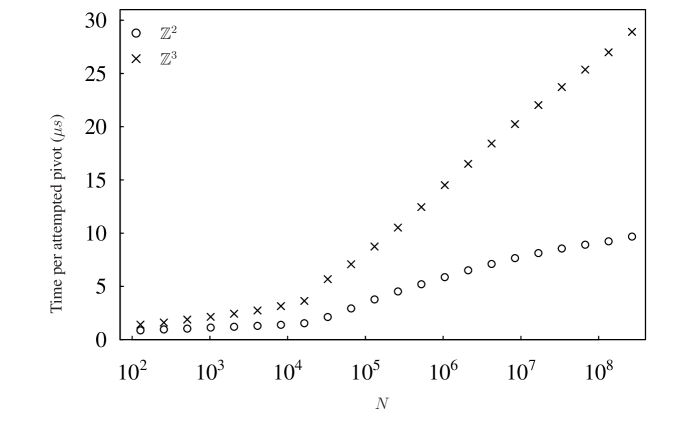
Figure 1: $T(N)$ for ${\mathbb{Z}}^{2}$ and ${\mathbb{Z}}^{3}$. Note that these estimates were obtained in a separate data run on a different computer from the main experiment, with lengths from $N=2^{7}-1$ to $N=2^{28}-1$.

For SAWs of length $N$, it is expected that the exponential autocorrelation time is approximately $O(N/f)$ Madras1988SAW , where $f$ is the fraction of pivot attempts which are successful. The first $20N/f$ configurations were discarded, ensuring that for all practical purposes SAWs were sampled from the uniform distribution. Batch estimates of $\langle R_{\mathrm{e}}^{2}\rangle_{33554431}$, using a batch size of $10^{8}$, are shown in Sec. 4 of Clisby2009bSAW ; in this case the first 50 batches were discarded, while initialization bias is visually apparent for (at most) the first 10 batches.

The computer experiment was performed on a cluster of AMD Opteron Barcelona 2.3GHz quad core processors, for a total of 16500 CPU hours. Code was written in C, and compiled with gcc. $10^{11}$ pivot attempts were made on SAWs of length ranging from 15 to $3.36\times 10^{7}$, for a grand total of $1.89\times 10^{13}$ pivot attempts. Data were collected from every pivot attempt for $f$ and the Euclidean-invariant moments $R_{x}^{2k}=\left(R_{x}^{2}\right)^{k}$ with $x\in\{\mathrm{e,g,m}\},1\leq k\leq 5$ . The longest walks with $N=3.36\times 10^{7}$ required 3GB of memory; much longer walks could conceivably be simulated in the future. By comparing fits from the whole data set ($N\leq 3.36\times 10^{7}$) with fits from a reduced data set ($N\leq 2.1\times 10^{6}$), we confirmed that data from the longest walks were indeed highly useful in tying down the various estimates (see Fig. 1 in Clisby2009aSAW ). However, the greatest benefit from the simulation of truly long walks, of say $10^{9}$ steps, may be the ability to directly simulate properties of realistic systems, such as DNA knotting, rather than determination of universal parameters.

Monte Carlo estimates of global parameters are collected in Tables II-V, Sec. 2 of Clisby2009aSAW , with confidence intervals calculated using the standard binning technique. For all lengths studied the integrated autocorrelation time of the Markov chain is much less than the batch size of $10^{8}$. We confirm the accuracy of the confidence interval estimates by studying the effect of batch size in Sec. 5 of Clisby2009bSAW .

II Analysis

We estimated the critical exponents $\nu$ and $\Delta_{1}\approx 1/2$ and associated amplitudes $D_{x}$ and $b_{x}$ by fitting the leading term and leading correction of Eq. (1) via weighted non-linear regression. We truncated the data set by requiring $N\geq N_{\mathrm{min}}$, with $N_{\mathrm{min}}$ a free parameter. We shifted the value of $N$ of Eq. 1 by an amount $\delta N_{x}$ to obtain smoother convergence by altering the sub-leading corrections (see e.g. Clisby2007SAW ); estimates for $\nu$, $\Delta_{1}$, $D_{x}$, and $b_{x}$ are unaffected in the limit $N_{\mathrm{min}}\rightarrow\infty$. With $\delta N_{\mathrm{e}}=.35$, $\delta N_{\mathrm{g}}=1$, $\delta N_{\mathrm{m}}=0.4$, our final model was

$$\langle R_{x}^{2}\rangle_{N} =D_{x}(N+\delta N_{x})^{2\nu}\left[1+\frac{b_{x}}{(N+\delta N_{x})^{\Delta_{1}}}\right],$$ (2)

Unfortunately we cannot fit the next-to-leading corrections with exponents $1$, $\Delta_{2}\approx 1$, and $2\Delta_{1}\approx 1$ as the differences between them are far too small to resolve. For sufficiently large $N_{\mathrm{min}}$ we found that reduced $\chi^{2}$ values for all fits approached 1 from above, indicating Eq. 2 is asymptotically correct.

Final estimates of parameters have been made directly from Figs. 2 and 3, combining multiple sources visually in an attempt to make estimates robust, and allow the reader to critically evaluate our final results. We do not distinguish between subjective and statistical errors, as we believe that in this context the distinction is itself quite subjective . We provide here some guidance for the interpretation of Figs. 2 and 3, and refer the interested reader to Guttmann1989Books for (much) more information on series analysis.

• We plot estimates against $N_{\mathrm{min}}^{-y}$, where $y$ is chosen such that $N_{\mathrm{min}}^{-y}$ is of the same order as the residual error from the fit. The estimates for $\Delta_{1}$ and $b_{x}$ have $y=1-\Delta_{1}\approx 0.47$, and $y=1$ for $\nu$ and $D_{x}$.

• We seek to extrapolate the fits to $N_{\mathrm{min}}=\infty$, or $N_{\mathrm{min}}^{-y}=0$. Depending upon whether the true value $y_{\mathrm{exact}}$ is less than, equal to, or greater than $y$, the estimates would approach a limiting value at $N_{\mathrm{min}}^{-y}=0$ with infinite, finite, or zero slope respectively.

• Successive estimates are highly correlated, and so any trend which lies within the error bars should be disregarded. Only some of the error bars are plotted in order to reduce visual noise.

• There are no bounds on the errors of the truncated asymptotic formulae, and hence the interpretation of the graphs is subjective. The underlying systematic error is observable dependent, and so combining estimates from a variety of observables improves robustness.

In Fig. 2 we plot estimates of $\Delta_{1}$ with our final result plotted at 0; the error bar reflects the scatter between observables. In Fig. 3 we plot estimates for $\nu$, biased with the lower and upper limits of our range for $\Delta_{1}$, with our final result at 0. Similar plots for the amplitudes are given in Figs. 5 and 6 of Clisby2009aSAW . We have conservatively chosen the error bar for the final result to encompass estimates from all observables $\langle R_{x}^{2}\rangle$. As the amplitudes $D_{x}$ are highly correlated with estimates for $\Delta_{1}$, the biasing of $\Delta_{1}$ greatly extends the range over which stable fits can be obtained. This is the reason the biased fits are preferred over the unbiased fits shown in Fig. 3 of Clisby2009aSAW .

Figure 2: Estimates for $\Delta_{1}$.

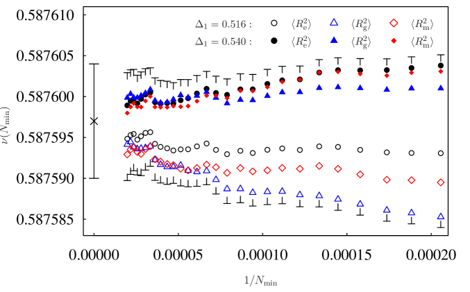
Figure 3: Estimates for $\nu$ from fits with biased $\Delta_{1}$. We show the envelope of maximum and minimum values of endpoints of error bars for all observables.

III Results

We report our final results in Table 2, and in addition we have $D_{\mathrm{m}}=0.58687(12)$, $b_{\mathrm{e}}=-0.49(5)$, $b_{\mathrm{g}}=-0.1125(125)$, and $b_{\mathrm{m}}=-0.295(30)$. If one assumes the hyperscaling relation $d\nu=2-\alpha$, then one also obtains $\alpha=0.237209(21)$. The estimates of $\nu$, $D_{\mathrm{e}}$, and $D_{\mathrm{g}}$ are in accordance with previous results, although considerably more accurate. The estimate for $\Delta_{1}$ is more accurate than the previous Monte Carlo value Li1995SAW , but less accurate than the Monte Carlo renormalization group estimate of Belohorec1997SAW , which relies upon an uncontrolled although accurate approximation. The claimed accuracy of the field theory estimates Guida1998SAW for $\Delta_{1}$ is also comparable, but as discussed by Li et al. Li1995SAW these calculations have underlying systematic errors of uncertain magnitude. Any desired amplitude ratios can be calculated from the amplitude estimates. The rational number with smallest denominator within 3 standard deviations of $\nu=0.587597$ is $161/274$, suggesting that $\nu$ cannot be expressed as a rational number with small denominator.

Table 2: Comparison of parameter estimates.

Source	$\nu$	$\Delta_{1}$	$D_{\mathrm{e}}$	$D_{\mathrm{g}}$
This Letter	0.587597(7)	0.528(12)	1.22035(25)	0.19514(4)
Clisby2007SAW Series	0.58774(22)		1.2178(54)
Prellberg2001SAW MC	0.5874(2)
MacDonald2000SAW Series	0.58755(55)		1.225
Guida1998SAW FT $d=3$	0.5882(11)	0.478(10)
Guida1998SAW FT $\epsilon$ bc	0.5878(11)	0.486(16)
Belohorec1997SAW MCRG	0.58756(5)	0.5310(33)
Li1995SAW MC	0.5877(6)	0.56(3)	1.21667(50)	0.19455(7)

We would like to stress that, due to the neglect of sub-leading terms, there are underlying systematic errors in our estimates which are not and cannot be controlled. We have the luxury of high quality data from long walks, and have attempted to be conservative with our claimed errors, but acknowledge there is a risk that the (subjective) confidence intervals may not be sufficiently large.

IV Conclusion

In summary, an efficient version of the pivot algorithm for SAWs has been implemented and used to calculate $\nu$; the algorithms developed promise to be widely useful in the Monte Carlo simulation of SAWs and related models of polymers.

- (1) Neal Madras and Gordon Slade. The Self-Avoiding Walk. Birkhaüser, Boston, 1993.
- (2) Bernard Nienhuis. Exact critical point and critical exponents of O() models in two dimensions. Phys. Rev. Lett., 49:1062–1065, 1982.
- (3) Gregory F. Lawler, Oded Schramm, and Wendelin Werner. On the scaling limit of planar self-avoiding walk. In Fractal Geometry and Applications: a Jubilee of Benoit Mandelbrot, Part 2. Proc. Sympos. Pure Math., volume 72, pages 339–364. Am. Math. Soc., Providence, 2004.
- (4) Takahashi Hara and Gordon Slade. Self-avoiding walk in five or more dimensions I. The critical behaviour. Commun. Math. Phys., 147:101–136, 1992.
- (5) Nathan Clisby. Fast implementation of the pivot algorithm for self-avoiding walks. J. Stat. Phys. (submitted), 2010.
- (6) Moti Lal. ‘Monte Carlo’ computer simulation of chain molecules. I. Mol. Phys., 17:57–64, 1969.
- (7) Neal Madras and Alan D. Sokal. The pivot algorithm: A highly efficient Monte Carlo method for the self-avoiding walk. J. Stat. Phys., 50:109–186, 1988.
- (8) Bin Li, Neal Madras, and Alan D. Sokal. Critical exponents, hyperscaling, and universal amplitude ratios for two- and three-dimensional self-avoiding walks. J. Stat. Phys., 80:661–754, 1995.
- (9) Tom Kennedy. A faster implementation of the pivot algorithm for self-avoiding walks. J. Stat. Phys., 106:407–429, 2002.
- (10) S. Müller and L. Schäfer. On the number of intersections of self-repelling polymer chains. Eur. Phys. J. B, 2:351–369, 1998.
- (11) Marco Baiesi, Enzo Orlandini, and Attilio L. Stella. Peculiar scaling of self-avoiding walk contacts. Phys. Rev. Lett., 87:070602, 2001.
- (12) Robert Sedgewick. Algorithms in C, Parts 1–4. Addison-Wesley, Reading, MA, 3rd ed., 1998.
- (13) Antonin Guttman. R-trees: A dynamic index structure for spatial searching. In SIGMOD ’84, pages 47–57. ACM Press, New York, 1984.
- (14) See supplementary material at http://link.aps.org/supplemental/10.1103/PhysRevLett.104.055702 for additional graphs and raw data. Free download from http://ftp.aip.org/epaps/phys_rev_lett/E-PRLTAO-104-055702/.
- (15) Nathan Clisby, Richard Liang, and Gordon Slade. Self-avoiding walk enumeration via the lace expansion. J. Phys. A: Math. Theor., 40:10973–11017, 2007.
- (16) A. J. Guttmann. Asymptotic analysis of power-series expansions. In Phase Transitions and Critical Phenomena, volume 13, pages 1–234. Academic Press, New York, 1989.
- (17) Peter Belohorec. Renormalization group calculation of the universal critical exponents of a polymer molecule. Ph.D. thesis, University of Guelph, 1997.
- (18) R. Guida and J. Zinn-Justin. Critical exponents of the -vector model. J. Phys. A: Math. Gen., 31:8103–8121, 1998.
- (19) T. Prellberg. Scaling of self-avoiding walks and self-avoiding trails in three dimensions. J. Phys. A: Math. Gen., 34:L599–L602, 2001.
- (20) D. MacDonald, S. Joseph, D. L. Hunter, L. L. Moseley, N. Jan, and A. J. Guttmann. Self-avoiding walks on the simple cubic lattice. J. Phys. A: Math. Gen., 33:5973–5983, 2000.