Witnessing the active assembly phase of massive galaxies since $z$ = 1

Abstract

We present an analysis of $\sim$60 000 massive (stellar mass $M_{\star}>10^{11}M_{\odot}$) galaxies out to $z=1$ drawn from 55.2 deg² of the United Kingdom Infrared Telescope (UKIRT) Infrared Deep Sky Survey (UKIDSS) and the Sloan Digital Sky Survey (SDSS) II Supernova Survey. This is by far the largest survey of massive galaxies with robust mass estimates, based on infrared ($K$-band) photometry, reaching to the Universe at about half its present age. We find that the most massive ($M_{\star}>10^{11.5}M_{\odot}$) galaxies have experienced rapid growth in number since $z=1$, while the number densities of the less massive systems show rather mild evolution. Such a hierarchical trend of evolution is consistent with the predictions of the current semi-analytic galaxy formation model based on $\Lambda$CDM theory. While the majority of massive galaxies are red-sequence populations, we find that a considerable fraction of galaxies are blue star-forming galaxies. The blue fraction is smaller in more massive systems and decreases toward the local Universe, leaving the red, most massive galaxies at low redshifts, which would support the idea of active ’bottom-up’ formation of these populations during $0<z<1$.

1 Introduction

Understanding the origin and evolution of galaxies, in particular the most massive, is one of the major challenges in modern astrophysics. Many massive galaxies today are giant early-type systems; hence the formation of spheroids should proceed to a certain extent in locked step with the mass assembly. The compelling theory of hierarchical galaxy formation predicts that galaxies are assembled through successive mergers of smaller systems in overdensities, or haloes, of hypothetical cold dark matter (CDM) (White & Rees, 1978). Massive galaxies therefore emerge in the last phase of the formation history. Alternatively, massive galaxies could form through the rapid collapse of gas followed by a single prominent starburst at high redshifts (Eggen, Lynden-Bell, & Sandage, 1962; Larson, 1975). This ’monolithic’ scenario is supported by, for example, the tight colour–luminosity relation of early-type galaxies found in galaxy clusters (e.g., Bower, Lucey, & Ellis, 1992; Ellis et al., 1997).

While different evolution in different models makes distant massive galaxies a unique test-bed for galaxy formation scenarios, observations have not yet provided evidence for the evolutionary path of those galaxies. The major obstacle in observations originates from the scarcity of galaxies at the high end of the galaxy mass function; it means that not only it is hard to find the population but also cosmic variance, the field-to-field variation of observed volume density arising from large-scale structure, is significant. In the last decade, many large programmes of optical-band imaging have been carried out, providing excellent data sets with which to investigate distant red old galaxies in wide fields of sky exceeding a whole deg² (e.g., Bell et al., 2004; Borch et al., 2006; Cimatti, Daddi, & Renzini, 2006; Willmer et al., 2006; Brown et al., 2007; Faber et al., 2007). They consistently suggest that the total stellar mass locked in red galaxies with luminosities around $L\sim L^{*}$, where $L^{*}$ is the characteristic luminosity of the luminosity function, has at least doubled since $z\sim 1$. Some of them also claim little growth in the number of very luminous galaxies well above $L\sim L^{*}$. However, while luminous red galaxies roughly correspond to massive galaxies, it is not clear how well the evolution in the number of galaxies at the steep high end of the mass function is understood from these results, since the much more numerous, less massive galaxies with mass-to-luminosity ratios slightly less than average could easily dominate the observed numbers of luminous galaxies. The above authors also reveal that a field of view of the order of a whole deg² is still not sufficient to conquer the uncertainty arising from cosmic variance for the high-end populations of the galaxy mass function.

The advent of the United Kingdom Infrared Telescope (UKIRT) InfraredDeep Sky Survey (UKIDSS; Lawrence et al., 2007) provides a unique opportunity to produce an ideal sample to trace various aspects of massive galaxies in the distant Universe. Here we report the results of a $K$-band survey with optical ($u$, $g$, $r$, $i$, $z$ band) and near-infrared ($Y$, $J$, $H$ band) photometry and optical spectra, focusing on massive ($M_{\star}>10^{11}M_{\odot}$) galaxies out to $z=1$ in an unprecedented large area covering 55.2 deg². The $K$-band photometry provides robust estimates of galaxy stellar masses (e.g., Matsuoka et al., 2008) while the very large field of view significantly suppresses cosmic variance, which allow us to conduct a unique analysis of the mean properties of distant massive galaxies.

This paper is organized as follows. In Section 2 we describe the data sources and reduction process to extract the galaxy sample from the available data. Photometric redshifts and stellar masses are measured for each galaxy in Section 3. In Section 4, the number-density evolution of massive galaxies and the associated uncertainties are explored. We then discuss the star-forming properties of galaxies and the compatibility of the present results with previous measurements in Section 5. A summary follows in Section 6. Throughout this paper, we adopt the concordance cosmology of $H_{0}$ = 70 km s^-1 Mpc^-1, $\Omega_{\rm M}=0.3$, and $\Omega_{\Lambda}=0.7$. Magnitudes are expressed in the Vega magnitude system for the UKIDSS near-infrared bands and in the AB magnitude system for the optical bands.

2 Data Sources and Reduction

2.1 Near-Infrared Photometry

We extract from the Data Release 3 (DR3; Warren et al., in preparation) of the UKIDSS/Large Area Survey (LAS) the $K$-band sources with right ascensions from 1^h 15^m to 3^h 6^m on the Sloan Digital Sky Survey (SDSS; York et al., 2000) southern equatorial stripe (see Section 2.2). The range in right ascension is chosen so that the $K$-band observations are fairly complete within the sample area. More than half of the $K$-band sources have also been observed in the $Y$, $J$ and/or $H$ bands. We exclude the sources assigned with serious quality flags corresponding to ppErrBits attributes larger than 31, or near (within 20 arcsec of) the detector edges of any exposure. We also exclude those sources near bright sources. This is achieved by searching for bright point and extended sources in the Two-Micron All-Sky Survey (2MASS; Skrutskie et al., 2006) catalogues and rejecting all the LAS sources within sufficiently large distances of the bright 2MASS sources. The total effective area of the observations defining our sample is 55.2 deg².

We retrieved all the images in our sample area from the DR3 data base, and used the SOURCE EXTRACTOR, version 2.5 (Bertin & Arnouts, 1996) for magnitude measurements. The total magnitudes ($m_{\rm tot}$) of the sources are measured with the SOURCE EXTRACTOR total magnitude algorithm MAG_AUTO. We measure the aperture magnitudes ($m_{\rm ap}$) with circular apertures of several diameters, 4.5, 3.3, 2.8 and 2.6 arcsec, which correspond to 20 kpc at $z$ = 0.3, 0.5, 0.7 and 0.9, respectively. Since the seeing condition is generally superior in the UKIDSS LAS ($\sim$0.8 arcsec) to that in the optical observations by the SDSS ($\sim$1.5 arcsec), the near-infrared images were smoothed with the Gaussian kernel in such a way that the resultant full widths at half-maximum (FWHMs) of stellar profiles are similar to those in the optical images of the same field. The seeing measurements and smoothing were performed in each of the small rectangular subareas of approximately 9 $\times$ 13 arcsec². Then we ran the SOURCE EXTRACTOR on the smoothed images to measure the aperture magnitudes of the sources.

The detection completeness of the $K$-band sources can be estimated by comparing the numbers of the LAS detections with those of the much deeper UKIDSS Deep Extragalactic Survey (DXS; Lawrence et al., 2007) in an overlapping field. This 0.6-deg² field is a part of the DXS VIMOS 4 field, which is centred at RA 22^h 17^m, Dec. $+$00^∘ 24’ on the celestial equator. While the field is outside the RA range of our LAS fields, we confirmed that the evaluation sample of this field has a similar distribution of magnitudes and their errors to those for our actual sample. Below we show that the derived detection-completeness function reproduces the galaxy number counts from our sample, in excellent agreement with previous measurements, while it gives the lower limit of the detection completeness for our massive galaxies. We define our sample as being brighter than the limiting total magnitude $K_{\rm tot}$ = 17.9 mag, where the detection completeness is higher than 0.5.

2.2 Optical Photometry

We use the optical $u$, $g$, $r$, $i$ and $z$-band images on the SDSS southern equatorial stripe. The stripe has been observed repeatedly in the SDSS-II Supernova Survey (Frieman et al., 2008) during 2005– 2007, as well as in the original SDSS. We retrieved all the available images taken on the stripe from the SDSS Data Release 6 Supplemental and Supernova Survey data bases (Adelman-McCarthy et al., 2008), and stacked them in each of the five bands. The images observed in runs 2738 and 3325 are set apart from others, since they are taken with the standard survey conditions of the original SDSS and can work as the reference frames for stellar photometry. We measure, for each retrieved image, the mean and root-mean-square (rms) of the sky counts and the sky transparency at the observation by comparing the stellar photometry of the relevant frame with that of the reference frames. After discarding the worst 5 per cent of the retrieved images with the largest rms of sky counts, which we find is sufficient to reject apparently flawed exposures, the images are zero-shifted and scaled according to the sky-count statistics and then stacked by the inverse-of-variance weighted average using IRAF. The photometric calibration of the stacked images is achieved by comparing the stellar photometry with that of the reference frames. We find that the stellar magnitudes on the stacked and reference frames are in excellent agreement, with rms less than 0.05 mag (Fig. 1). Fig. 2 shows the comparison of the original and stacked r-band images of the same field. More than 100 original SDSS frames contribute to each of the stacked frames, and the latter images are on average $>$2mag deeper than the former images.

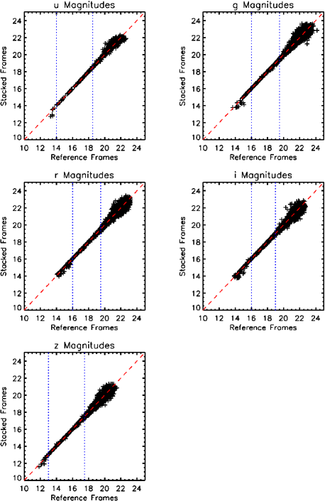
Figure 1: Comparisons of stellar magnitudes in the stacked and reference frames in $u$ (top left), $g$ (top right), $r$ (middle left), $i$ (middle right) and $z$ (bottom left) bands. The dashed lines represent the locus where the two measurements are identical. The rms errors of the photometric calibration are calculated in the magnitude ranges shown by the dotted lines, where the stellar photometry is most reliable.

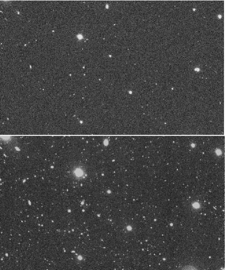
Figure 2: Original (top) and stacked (bottom) SDSS $r$-band images of the same field.

We run the SOURCE EXTRACTOR on the stacked images to extract detected sources. The groups with four or more pixels whose counts are 1.5$\sigma$ above the local background level are identified as sources. For every detection, we measure the aperture magnitudes in the 4.5-, 3.3-, 2.8- and 2.6-arcsec diameter apertures as we did for the near-infrared images. The photometry errors are calculated from the source photon counts and the background noise. The extracted sources are cross-identified with the $K$-band sources within the maximum paring tolerance of 1.0 arcsec. Owing to the deep stacking of the SDSS images, nearly 90 per cent of the $K$-band sources have counterparts in the $g$, $r$, $i$ and $z$ bands. Nearly 40 per cent of the $K$-band sources also have counterparts in the $u$ band.

2.3 Optical Spectroscopy

We exploit the two redshift surveys carried out on the SDSS southern equatorial stripe; the VIMOS-VLT Deep Survey (VVDS; Le Fèvre et al., 2005) and the DEEP2 Redshift Survey (Davis et al., 2003). Among the four fields of the VVDS ’Wide’ survey, we use the 4-deg² field of the F22 (2217$+$00), which lies on the celestial equator, centred at RA 22^h 17^m 50^s.4 and Dec. $+$00^∘ 24^m 00^s. This field coincides with the UKIDSS DXS VIMOS 4, and is observed in both the LAS and the DXS. We use Field 4 (RA 02^h 30^m, Dec. $+$00^∘ 00^m) of the DEEP2, one of the ’1-h survey’ fields placed on our LAS field. The VVDS adopts a pure $I$-band flux-limited selection of the sample while the DEEP2 imposes strict colour pre-selection on the spectroscopic targets to favour galaxies at $z>0.7$; thus the two surveys are complementary in terms of the sample selection. We use only the spectroscopic sample with high redshift-quality flags, zflag/zQ = 3 or 4 for the VVDS/DEEP2. As a result, we obtain 253 LAS $K$–VVDS and 375 LAS $K$–DEEP2 galaxies, as well as 1084 DXS $K$–VVDS galaxies. We note that the redshift surveys are deep enough that essentially all the LAS $K$ sources could be sampled.

2.4 Star/Galaxy Classification

The $K$-band sources separate clearly into stars and galaxies on the $r-z$ versus $z-K$ diagram as shown in Fig. 3. The colours are measured with the 2.8-arcsec diameter aperture magnitudes. We define the demarcation between stars and galaxies along the minimum surface density on this diagram, i.e. the sources redder than $z-K=0.52(r-z)+1.74$ are classified as galaxies. The additional criterion of $r-z<4$ is set for galaxies to exclude cool dwarf stars from the sample. We obtain 259 082 galaxies with these classification criteria. The VVDS classification based on spectra confirms that the above scheme works very well, yielding a rate of misclassification (stars classified as galaxies and vice versa) of less than $\sim$1 per cent. The $K$-band sources without $r$- and/or $z$-band detections are excluded from the sample, since their extremely red colours suggest that they are mostly galaxies beyond $z=1$. Actually, we find that more than 95 per cent of the LAS $K$–VVDS and LAS $K$–DEEP2 galaxies are detected in both $r$ and $z$ bands in any redshift bins at $z\leq 1$.

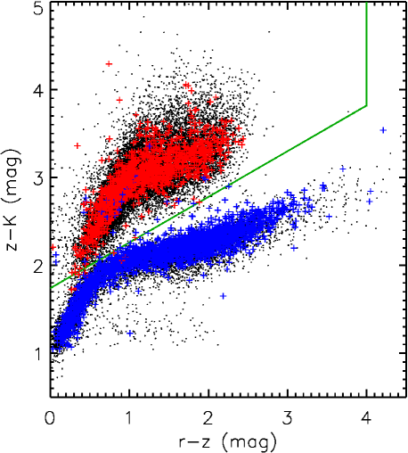
Figure 3: The $r-z$ versus $z-K$ diagram for a subset of $K$-band sources (black), on which the VVDS stars (blue) and galaxies (red) are superimposed. The green line represents the adopted star/galaxy classification criteria.

We show the $K$-band differential number counts of the extracted galaxies in Fig. 4. They are in excellent agreement with previous measurements (Daddi et al., 2000; Huang et al., 2001) down to the limiting magnitude of $K_{\rm tot}$ = 17.9 mag after the detection-completeness correction is applied. This suggests that we have successfully constructed a well-defined sample of galaxies through the above processes.

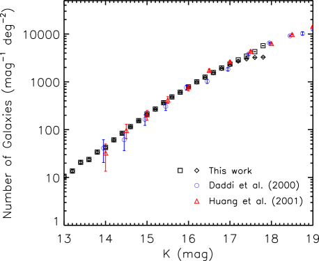
Figure 4: The $K$-band differential number counts of the extracted galaxies with (squares) and without (diamonds) detection-completeness correction. The error bars denote Poisson noise. The blue circles and the red triangles represent the measurements of Daddi et al. (2000) and Huang et al. (2001), respectively.

3 Redshift and Stellar mass Measurements

3.1 Photometric Redshift

We estimate the redshifts of galaxies from the observed broad-band colours, measured in the 2.8-arcsec diameter aperture, with the optimized template-fitting method following Ilbert et al. (2006). We present a short summary of the method below, while the full description of the concept and details can be found in the above reference.

We choose the DXS $K$–VVDS galaxies to optimize the spectral templates, leaving the LAS $K$–VVDS and LAS $K$–DEEP2 galaxies as the evaluation sets of the redshift measurements (Table 1). First, the DXS $K$–VVDS galaxies are classified into five spectral types, Ell, Sbc, Scd, Irr and starburst (SB) by least-$\chi^{2}$ fitting with the appropriate amounts of dust extinction assuming the extinction laws of the Small Magellanic Cloud (SMC) by Pei (1992) for Scd and Irr and that of starburst galaxies by Calzetti et al. (2000) for SB. The initial spectral templates are taken from Coleman, Wu, & Weedman (1980) for Ell, Sbc, Scd and Irr and from Kinney et al. (1996) for SB. Then, for each filter $f$, we minimize the sum

$$\psi^{2}=\sum_{\rm galaxy}\biggl{(}\frac{F_{\rm obs}^{f}-A\times F_{\rm model}^{f}-s^{f}}{\sigma_{\rm obs}^{f}}\biggr{)}^{2},$$ (1)

where $F_{\rm obs}^{f}$ and $\sigma_{\rm obs}^{f}$ are the observed flux and its error in the filter $f$. The sum is taken over all the sample galaxies. The parameters $F_{\rm model}^{f}$ and $A$ represent the best-fitting template flux and its normalization factor taken from the initial least-$\chi^{2}$ fitting. The last term $s^{f}$ is a free parameter. While this term should be zero in the case of a completely random uncertainty in the photometry, we find that it has a non-zero value in every filter. These values are at most 0.05 mag and are comparable with the expected uncertainty in the photometric zero-point calibration.

Table 1: Summary of the spectroscopic sample.

Sample	Number	Use∗1
DXS $K$ – VVDS	1084	training
LAS $K$ – VVDS∗2	253	evaluation
LAS $K$ – DEEP2	375	evaluation

^∗1Use in the photometric-redshift measurements.
^∗2Approximately 70% of the LAS $K$ – VVDS galaxies are also the members of the DXS $K$ – VVDS galaxies.

The DXS $K$–VVDS galaxies are re-classified into five spectral-type groups with the terms $s^{f}$ considered. In each group, the observed broad-band fluxes of galaxies are converted to the rest frame according to the spectroscopic redshifts, after being normalized and de-reddened by the best-fitting normalization factor $A$ and the dust extinction. Since the galaxies have various redshifts, this conversion generates a continuous spectral energy distribution for each spectral type of galaxies over the relevant rest-frame wavelength range. We sort the rest-frame fluxes according to their wavelengths and bin them by groups of points, and connect the median flux in each bin to produce the optimized templates. We keep the extrapolations provided by the initial templates in ultraviolet and infrared wavelengths where no broad-band data are available. The starburst template is not optimized, in order to retain the emission lines in the template. Finally, these optimized templates are interpolated to produce a total of 62 templates, the first being Ell and the last being SB, to improve the sampling of the redshift–colour space. Below we define the spectral type of each galaxy using the best fits from among these 62 templates.

The created spectral templates are fitted to the observed colours of the actual sample to measure their redshifts. We evaluate the measurement accuracy by applying the same procedure to the LAS $K$–VVDS and LAS $K$–DEEP2 galaxies, as well as the DXS $K$–VVDS galaxies. The DXS $K$–VVDS galaxies are reduced in number according to the LAS $K$-band detection completeness and are given additional random photometry errors in order to simulate the LAS $K$-band galaxies.We find that the photometric redshifts ($z_{\rm phot}$) are well correlated with the spectroscopic redshifts ($z_{\rm spec}$) as shown in Fig. 5, thanks to our wide and relatively fine wavelength coverage in the $u$ through $K$ bands. The deviation between the two (photometric and spectroscopic) measurements closely follows a Gaussian distribution with standard deviation $\sigma_{{\Delta}z/(1+z)}\sim 0.04$ (${\Delta}z=z_{\rm spec}-z_{\rm phot}$) for all three sets of the evaluation sample. Note that $\sim$70 per cent of the LAS $K$–VVDS galaxies are also members of the DXS $K$–VVDS galaxies and account for about a quarter of the sample used to build up the spectral templates, so that the LAS $K$–VVDS galaxies do not provide a completely independent test of the photometric-redshift accuracy. As a further test, we created another template set from the DXS $K$–VVDS galaxies omitting these LAS $K$–VVDS galaxies and repeated the photometric-redshift measurement. This test again gives $\sigma_{{\Delta}z/(1+z)}\sim 0.04$, which indicates that it is a robust estimate of the photometric-redshift uncertainty. We show the uncertainty as a function of redshift and stellar mass (as determined below) in Table 2. They are relatively large in the lowest and highest redshift bins for larger stellar mass classes, for which relatively small numbers of sample contribute to the spectral templates. We also show the uncertainty as a function of spectral type in Table 3, which suggests there is little variation of uncertainty among the different spectral types.

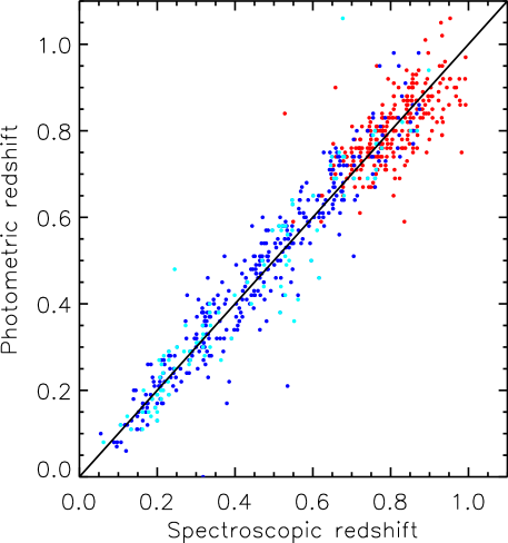
Figure 5: Comparison of the photometric and spectroscopic redshift measurements of LAS $K$–VVDS (light blue), DXS $K$–VVDS (blue) and LAS $K$–DEEP2 (red) galaxies. The solid line shows the locus where the two measurements are identical.

Table 2: Uncertainty ($\sigma_{{\Delta}z/(1+z)}$) in photometric redshift.

		log $M_{\star}$
Redshift	10.0 – 10.5	10.5 – 11.0	11.0 – 11.5	11.5 – 12.0
0.2 – 0.4	0.037 (50)	0.046 (51)	0.043 ( 6)	— ( 0)
0.4 – 0.6	0.040 (35)	0.037 (55)	0.039 (25)	— ( 0)
0.6 – 0.8	0.021 (35)	0.030 (73)	0.032 (93)	0.034 (20)
0.8 – 1.0	0.033 (17)	0.038 (71)	0.046 (55)	0.047 ( 7)

Note — Numbers in parentheses represent the number in the evaluation samples.

Table 3: Uncertainty ($\sigma_{{\Delta}z/(1+z)}$) in photometric redshift.

Spectral type	$\sigma_{{\Delta}z/(1+z)}$
Ell – Sbc	0.035 (386)
Sbc – Scd	0.037 (171)
Scd – Irr	0.036 ( 35)
Irr – SB	— ( 0)

Note — Numbers in parentheses represent the number in the evaluation samples.

3.2 Stellar Mass

The stellar masses ($M_{\star}$) of galaxies are determined by fitting to the observed colours the stellar population synthesis models of Bruzual & Charlot (2003). The aperture magnitudes ($m_{\rm ap}$) of the 4.5-, 3.3-, 2.8- and 2.6-arcsec apertures are used for the fitting of galaxies with photometric redshifts $z$ = 0.2–0.4, 0.4–0.6, 0.6–0.8, and 0.8–1.0, respectively, so that we sample the stellar populations consistently within the central $\sim$20 kpc of all the galaxies. The resultant stellar mass is then scaled by $10^{0.4(K_{\rm ap}-K_{\rm tot})}$ to correct for aperture loss. We adopt the standard configurations with the Padova 1994 stellar evolutionary tracks and BaSel 3.1 spectral library for the Bruzual & Charlot (2003) models. We assume three values of metallicity: 0.2, 1 and 2.5 $Z_{\odot}$, where $Z_{\odot}$ is the solar metallicity. The star-formation history is assumed to take the exponentially declining form $\tau^{-1}$ exp($-t/\tau$), where the $e$-folding time $\tau$ is a free parameter, with the Salpeter (1955) initial mass function (IMF). Our stellar mass estimates can be approximately converted to those with another commonly used IMF, that of Chabrier (2003), by adding $\sim$0.25 dex. Other free parameters are the age $t$ of the stellar population and the colour excess $E(B-V)$ due to the dust extinction of the stellar radiation, following the SMC extinction curve of Pei (1992). These parameters are varied over the plausible ranges of 10 Myr $\leq\tau\leq$ 10 Gyr ($\Delta$log $\tau$ = 0.2), 10 Myr $\leq t\leq$ 10 Gyr ($\Delta$log $t$ = 0.1), and $0.0\leq E(B-V)\leq 0.5$ mag ($\Delta$$E(B-V)$ = 0.05), and the best-fitting parameter set is searched for by the least-$\chi^{2}$ method for each galaxy (the values in parentheses represent the grid intervals). The additional error of 0.05 mag is added in quadrature to all band magnitudes in the fitting in order to take into account the uncertainty in the photometric zero-point calibration.

We derive two kinds of stellar mass for the spectroscopic sample, i.e. the stellar mass with spectroscopic redshifts ($M_{\star,spec}$) and the stellar mass with photometric redshifts ($M_{\star,phot}$). The difference between the two measures, $\Delta{\rm log}M_{\star}={\rm log}M_{\star,spec}-{\rm log}M_{\star,phot}$, is found to be clearly correlated with the photometric redshift deviation ${\Delta}z=z_{\rm spec}-z_{\rm phot}$. Such a correlation is expected, since a larger $z_{\rm phot}$ leads to a larger estimate of the galaxy luminosity, which then leads to a larger estimate of stellar mass $M_{\star,phot}$. The observed relation between ${\Delta}z$ and $\Delta{\rm log}M_{\star}$ is actually quite consistent with this expected correlation. Another expected cause of the correlation between ${\Delta}z$ and $\Delta{\rm log}M_{\star}$ comes from the fact that larger estimates of $z_{\rm phot}$ lead to systematically shorter rest-frame wavelengths to which each of the observing wavebands corresponds. After removal of the above first component of the systematic correlation, we found marginal evidence for the second correlation in our sample, which is $\Delta{\rm log}M_{\star}$ = $+/-$ ($0.04\pm 0.07$) when ${\Delta}z$ is negative/positive. In addition, we consider the uncertainty associated with the least-$\chi^{2}$ model fitting. It is evaluated by the 1$\sigma$ confidence surface of the $\chi^{2}$ distributions in the fitting parameter space.

We show the total amplitudes of the stellar mass uncertainty ($\sigma_{\Delta{\rm log}M_{\star}}$) as a function of redshift and stellar mass in Table 4. Those as a function of spectral type are shown in Table 5. The above estimates of error amplitudes and the correlations between ${\Delta}z$ and $\Delta{\rm log}M_{\star}$ are taken into account in the Monte Carlo simulation presented below. Note that further different assumptions on the stellar mass estimation, such as different stellar population synthesis models and different IMF, can cause additional uncertainty in the derived properties of galaxies. We will address this issue in Section 5.

Table 4: Uncertainty ($\sigma_{\Delta{\rm log}M_{\star}}$) in stellar mass.

		log $M_{\star}$
Redshift	10.0 – 10.5	10.5 – 11.0	11.0 – 11.5	11.5 – 12.0
0.2 – 0.4	0.19 (50)	0.20 (51)	0.22 ( 6)	— ( 0)
0.4 – 0.6	0.19 (35)	0.17 (55)	0.16 (25)	— ( 0)
0.6 – 0.8	0.12 (35)	0.16 (73)	0.17 (93)	0.19 (20)
0.8 – 1.0	0.14 (17)	0.17 (71)	0.19 (55)	0.25 ( 7)

Note — Numbers in parentheses represent the number in the evaluation samples.

Table 5: Uncertainty ($\sigma_{\Delta{\rm log}M_{\star}}$) in stellar mass

Spectral type	$\sigma_{\Delta{\rm log}M_{\star}}$
Ell – Sbc	0.16 (386)
Sbc – Scd	0.17 (171)
Scd – Irr	0.17 ( 35)
Irr – SB	— ( 0)

Note — Numbers in parentheses represent the number in the evaluation samples.

4 Results

We define our massive galaxy sample using two stellar mass classes, i.e. $10^{11.0-11.5}M_{\odot}$ galaxies with $10^{11.0}M_{\odot}<M_{\star}<10^{11.5}M_{\odot}$ and $10^{11.5-12.0}M_{\odot}$ galaxies with $10^{11.5}M_{\odot}<M_{\star}<10^{12.0}M_{\odot}$. The galaxies are grouped into four redshift bins, $z$ = 0.2 – 0.4, 0.4 – 0.6, 0.6 – 0.8, and 0.8 – 1.0. Total numbers included in the sample are summarized in Table 6. The median photometry errors in the $r$-, $z$-, and $K$-band aperture magnitudes and in the $K$-band total magnitudes ($r_{\rm ap}$, $z_{\rm ap}$, $K_{\rm ap}$, $K_{\rm tot}$) are also listed. The aperture magnitude errors are generally smaller than the typical uncertainty in the photometric zero-point calibration ($\sim$0.05 mag).

Table 6: Summary of the massive galaxy sample.

	log $M_{\star}$ =	11.0 – 11.5	log $M_{\star}$ =	11.5 – 12.0
Redshift	Number	Photometry Error∗	Number	Photometry Error∗
0.2 – 0.4	9,720	($<$0.01, $<$0.01, 0.01, 0.05)	1,408	($<$0.01, $<$0.01, $<$0.01, 0.03)
0.4 – 0.6	15,300	($<$0.01, $<$0.01, 0.02, 0.08)	572	($<$0.01, $<$0.01, 0.01, 0.04)
0.6 – 0.8	18,582	(0.02, 0.02, 0.03, 0.13)	815	(0.01, 0.01, 0.02, 0.09)
0.8 – 1.0	12,371	(0.04, 0.02, 0.04, 0.16)	613	(0.03, 0.02, 0.03, 0.12)

Note (^∗) — Median photometry errors in the r-, z- and K-band aperture magnitudes and in the K-band total magnitudes ($r_{\rm ap}$, $z_{\rm ap}$, $K_{\rm ap}$, $K_{\rm tot}$).

We show the differential number counts of the massive galaxies in Fig. 6. It shows that the number-count distributions of the $10^{11.5-12.0}M_{\odot}$ galaxies have faint-end drop-offs at magnitudes brighter than the limiting magnitude, which assures the near-complete detection of this population. On the other hand, the faintest of the $10^{11.0-11.5}M_{\odot}$ galaxies at high redshifts ($z>0.6$) fall below the limiting magnitude, and are thus left uncounted. In order to estimate the lost fraction of $10^{11.0-11.5}M_{\odot}$ galaxies at these redshifts, we derive the detection completeness specifically for these galaxies as follows. We take each of the $10^{11.0-11.5}M_{\odot}$ galaxies in the lowest redshift bin and assign random redshifts in the $0.6<z<0.8$ and $0.8<z<1.0$ ranges. The galaxies are dimmed and reduced in apparent size according to the assigned redshifts, placed on random positions of the LAS $K$-band images, and then extracted by SOURCE EXTRACTOR in the same way as the actual sample sources are detected. The recovery rate of the embedded objects as a function of their magnitudes gives the detection completeness of the galaxies, which we find is significantly better than that of the whole sample derived before. The 50 per cent detection completeness is actually achieved at $K_{\rm tot}$ = 18.6 mag instead of $K_{\rm tot}$ = 17.9 mag, and almost all galaxies brighter than $K_{\rm tot}$ = 17.9 mag are detected. With the new detection-completeness function taken into account, the fractions of $10^{11.0-11.5}M_{\odot}$ galaxies fainter than the formal limiting magnitude ($K$ = 17.9 mag, thus uncounted) are 11 and 16 per cent at $z$ = 0.6–0.8 and 0.8–1.0, respectively

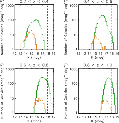
Figure 6: The differential number counts of $10^{11.0-11.5}M_{\odot}$ (green) and $10^{11.5-12.0}M_{\odot}$ (orange) galaxies at $z$ = 0.2–0.4 (top left), 0.4–0.6 (top right), 0.6–0.8 (bottom left) and 0.8–1.0 (bottom right). The black dashed lines represent our formal limiting magnitude of $K_{\rm tot}$ = 17.9 mag.

We estimate the uncertainty in the measured numbers of massive galaxies by a Monte Carlo simulation, as follows. First, we generate a mock galaxy catalogue containing 10 galaxies for each stellar mass ($\Delta$log$M_{\star}=0.1$) and redshift ($\Delta{z}=0.02$) bin in the ranges $8.0<$ log $M_{\star}$ $<13.0$ and $0.0<z<1.4$, where the numbers in parentheses represent the bin widths. Each galaxy is assigned a weighting factor corresponding to the number density of galaxies, following the galaxy mass function of Cole et al. (2001). Next the redshifts of galaxies are given perturbations following the measured uncertainty of the actual sample. The stellar masses are also given perturbations, correlated with the photometric redshift perturbations as explored in Section 3.2. Then the mock galaxies are weighted by their weighting factors and redistributed, and counted in the redshift and stellar mass bins to obtain the output mass function. We repeat the calculation 100 times, varying the random components.

Fig. 7 shows the results of the simulation. We observe both systematic and random components in the resultant error estimates. The systematic component is evident in $M_{\star}>10^{12.0}M_{\odot}$ bins. This is the so-called Eddington bias (Eddington, 1913), caused by the steep slope of the high end of the mass function; simply put, a small portion of the less massive, much more numerous galaxies could contaminate the more massive classes owing to measurement errors, which significantly alters the steep part of the mass function. This is why we limit our massive galaxy sample to those with $M_{\star}<10^{12.0}M_{\odot}$; the systematic increases in number are found to be insignificant for our mass ranges, i.e. negligible for the $10^{11.0-11.5}M_{\odot}$ galaxies and 40–60 per cent for the $10^{11.5-12.0}M_{\odot}$ galaxies. The output number densities from the 100 repeated calculations scatter around the systematic components, which yields the random components of the measurement error. The standard deviations of the scatter are $\sim$5 per cent and $\sim$12 per cent of the numbers of $10^{11.0-11.5}M_{\odot}$ and $10^{11.5-12.0}M_{\odot}$ galaxies, respectively. Note that the current estimate is not perfect, since we assume a non-evolving galaxy stellar mass function at $0<z<1$, while our results show clear signs of its evolution (see below). We will discuss this issue further in the following section.

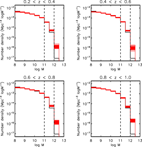
Figure 7: The input (black line) and output (100 red lines) galaxy mass functions of the Monte Carlo simulation at $z$ = 0.2–0.4 (top left), 0.4–0.6 (top right), 0.6–0.8 (bottom left) and 0.8–1.0 (bottom right). The dashed lines show the mass ranges in which our massive galaxy sample is defined.

Another source of uncertainty comes from cosmic variance. We estimate cosmic variance by dividing our sample into five subfields along the right ascension, $\sim$11 deg² each, and then calculating the fractional variation of the measured numbers of massive galaxies in these subfields. We find that the fractional variations are $<$10 per cent and $<$20 per cent for the $10^{11.0-11.5}M_{\odot}$ and $10^{11.5-12.0}M_{\odot}$ galaxies, respectively, in each of the four redshift bins. Considering that the total fields are five times larger than the subfields, we conclude that cosmic variance could affect the measured number of massive galaxies in each redshift bin by up to 5 per cent and 10 per cent for the two classes of galaxies, respectively. The above estimates are roughly consistent with the theoretical predictions provided by Somerville et al. (2004).

We show our results with regard to the number-density measurements in Table 7, and plot them along with the measurements for the local Universe (Cole et al., 2001) in Fig. 8. The error bars take into account all uncertainties considered above, as well as the Poisson noises. The number densities of the $10^{11.5-12.0}M_{\odot}$ galaxies are corrected for Eddington bias, although this correction has little significance for our final conclusions. The local densities were normalized to take into account the assumptions of Cole et al. (2001) with regard to stellar population synthesis that differ from ours; the major difference is that they assume a constant formation redshift of galaxies at $z_{f}=20$, while we vary the age of the stellar population as a free parameter. The normalization factor, $\sim 0.4$, is derived by applying their assumption to our $10^{11.0-11.5}M_{\odot}$ galaxies in the lowest redshift bin $z$ = 0.2–0.4. As seen in the figure, we find that the most massive ($10^{11.5-12.0}M_{\odot}$) galaxies have experienced rapid evolution in number since $z=1$. On the other hand, the number densities of the less massive ($10^{11.0-11.5}M_{\odot}$) systems show a rather mild evolution during the same period.

Table 7: Number densities of the massive galaxies.

	log $M_{\star}$
Redshift	11.0 – 11.5	11.5 – 12.0
0.2 – 0.4	10.9 $\pm$ 0.8	0.98 $\pm$ 0.15
0.4 – 0.6	7.8 $\pm$ 0.6	0.19 $\pm$ 0.03
0.6 – 0.8	6.8 $\pm$ 0.5	0.17 $\pm$ 0.03
0.8 – 1.0	3.7 $\pm$ 0.3	0.11 $\pm$ 0.02

Note — Number densities are given in units of $10^{-4}$ Mpc^-3 log $M_{\star}^{-1}$.

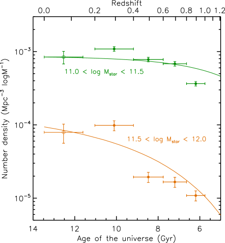
Figure 8: The number densities of massive galaxies versus the age of the Universe or redshift. The green and orange symbols and lines represent the $10^{11.0-11.5}M_{\odot}$ and $10^{11.5-12.0}M_{\odot}$ galaxies, respectively. The filled circles represent our measurements while the open circles represent measurements in the local Universe (Cole et al., 2001). The solid lines represent the predictions of the Millennium Simulation with the semi-analytic galaxy formation model (see text).

5 Discussion

The measured number density evolution of massive galaxies shows clear signs of the hierarchical evolution of these systems. Such a galaxy evolution scenario is predicted in the latest galaxy formation models based on $\Lambda$CDM theory. In Fig. 8 we overlay the predictions of the Millennium Simulation (Lemson et al. 2006), the largest numerical simulation to date based on $\Lambda$CDM theory, with the semianalytic galaxy formation model of De Lucia & Blaizot (2007), scaled to fit to the local observations (by a factor of 0.4). The stellar mass of the Millennium model has been shifted by $+$0.25 dex in order to correct for the different IMFs adopted (the model adopts the Chabrier (2003) IMF). The observed hierarchical pattern of evolution is consistent with the prediction of the model, while we find some discrepancies between the observation and the model (e.g. the $10^{11.0-11.5}M_{\odot}$ galaxies at $z$ = 0.8–1.0). This indicates that the basic idea of the bottom-up construction of galaxy systems is valid at least for the most massive galaxies with $M_{\star}>10^{11}M_{\odot}$.

Meanwhile, we point out that our measurements plotted in Fig. 8 seem to have an apparently unnatural feature at $z$ = 0.2–0.4, where the number densities are significantly high relative to the overall trend considering their estimated errors, implying residual systematic effects from the Eddington bias. We check this by investigating the systematic increases in the number of massive galaxies in the spectroscopic sample, from those obtained with the spectroscopic redshifts to those with photometric redshifts (we consider only those redshift and stellar mass classes with more than five spectroscopic sources). The above Monte Carlo simulation shows that the use of photometric redshifts (and the consequent stellar mass fluctuations) is the dominant source of the Eddington bias. We list the measured systematic increases in Table 8 separately for the VVDS and DEEP2 galaxies, since the amplitudes of the Eddington bias are subject to the redshift distribution of sources. The DXS $K$–VVDS galaxies have been given additional photometry errors and detection incompleteness in order to simulate the LAS $K$ galaxies. The systematic increases estimated in the Monte Carlo simulation are also listed in Table 8. The table shows that the systematic increases measured in the spectroscopic sample are mostly less than the estimates from the Monte Carlo simulation, while the one for the VVDS $10^{11.0-11.5}M_{\odot}$ galaxies at $z=0.2-0.4$ is exceptionally high. While it is based on a small sample, it provides marginal evidence that the Eddington bias is unexpectedly significant in this lowest redshift bin, due to some unquantified sources of systematic uncertainty. In that case, the number densities measured at $z$ = 0.2–0.4 should be regarded as the upper limits.

We also note that we adopt a non-evolving galaxy stellar mass function in the Monte Carlo simulation, while our results suggest the steepening of the high end of the mass function toward high redshifts; thus the estimated amount of Eddington bias should be regarded as a lower limit. When such a steepening of the mass function is taken into account in the correction of the Eddington bias, we obtain even lower numbers of galaxies in the more massive classes at higher redshifts, which would further strengthen our conclusion.

Table 8: Estimates of the Eddington bias^∗1.

	log $M_{\star}$ =	11.0 – 11.5		log $M_{\star}$ =	11.5 – 12.0
Redshift	MCS∗2	VVDS∗3	DEEP2∗3	MCS∗2	VVDS∗3	DEEP2∗3
0.2 – 0.4	$<$ 0.1	0.7 (6)	- (0)	0.6	- (0)	- (0)
0.4 – 0.6	$<$ 0.1	$<$ 0.1 (23)	- (2)	0.5	- (0)	- (0)
0.6 – 0.8	0.1	0.1 (21)	$<$ 0.1 (72)	0.6	0.3 (7)	0.3 (13)
0.8 – 1.0	$<$ 0.1	- (2)	$<$ 0.1 (53)	0.4	- (0)	0.1 (7)

^∗1Rates of increase (increased amounts divided by the original values) of the number densities are listed.

^∗2Estimates from the Monte Carlo simulation.

^∗3Estimates from the VVDS and DEEP2 spectroscopic samples (the number in the samples is shown in the parentheses).

Recently, Marchesini et al. (2009) provided a detailed analysis of random and systematic uncertainties affecting the galaxy stellar mass function. They adopt 14 different stellar mass estimations with different combinations of metallicity, dust extinction law, stellar population synthesis models and IMF, and show that the derived number density of galaxies in a given stellar mass bin could be altered by up to 1 dex. The ’bottom-light’ IMFs in particular, with a deficit of low-mass stars relative to a standard Chabrier (2003) IMF, give significantly different results for the stellar mass function from other classical IMFs. A more top-heavy IMF at higher redshifts is actually suggested by, for example, Davé (2008) and van Dokkum (2008). Thus we point out that our results are subject to a systematic change of these stellar-population properties during $0<z<1$. Future improvements in stellar population models based on new observations are eagerly awaited to overcome these large uncertainties inherent in stellar mass measurements.

In order to probe the star-forming properties of massive galaxies, here we investigate their rest-frame optical colours. Nearby galaxies are known to show a clear bimodality in the optical colour distribution, in which early-type galaxies form a narrow red sequence that is separated from blue star-forming populations by a valley of the galaxy distribution (e.g., Strateva et al., 2001; Hogg et al., 2003). A similar bimodality is observed out to $z>1$ (e.g., Lin et al., 1999; Im et al., 2002; Bell et al., 2004). We calculate the rest-frame $U$- and $V$-band magnitudes of massive galaxies by $k$-correcting the nearest observed $r$, $i$ or $z$-band magnitudes, where the amounts of the $k$-corrections are estimated from the best-fitting spectral population synthesis models. We show the resultant colour distributions in Fig. 9.

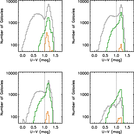
Figure 9: $U-V$ colour distributions of the massive galaxies at $z$ = 0.2–0.4 (top left), 0.4–0.6 (top right), 0.6–0.8 (bottom left) and 0.8–1.0 (bottom right). The grey, green and orange lines represent the $<10^{11.0}M_{\odot}$, $10^{11.0-11.5}M_{\odot}$ and $10^{11.5-12.0}M_{\odot}$ galaxies, respectively. The dotted lines show the demarcation between the blue and red populations.

As Fig. 9 shows, the less massive ($<10^{11.0}M_{\odot}$) galaxies show a clear colour bimodality, as expected, with the peak colour of the red sequence at $U-V\sim 1.2$ and a valley of galaxy distributions at $U-V\sim 1.0$ in all redshift bins. Compared with these galaxies, massive ($>10^{11.0}M_{\odot}$) galaxies are apparently dominated by the red population, with conspicuous peaks at $U-V\sim 1.2$. We divide the galaxies into blue and red populations at $U-V=1.0$ and calculate the blue fractions (fractions of the blue population). The associated errors are estimated by repeatedly giving random fluctuations to the $U-V$ colours, taking into account the uncertainties in the photometry and the amount of $k$-correction, and then re-measuring the blue fractions. We find that the fluctuated blue fractions are systematically larger than the original values, since there is a greater red population than blue around the demarcation $U-V=1.0$, and correct for the effect (the correction amounts are included in the final errors). We plot the measured blue fractions as a function of redshift and stellar mass in Fig. 10, and also list them in Table 9. One can see that the blue fractions are significantly lower in more massive galaxies, and that the fractions in massive systems decrease toward the local Universe. The blue fractions in $<10^{11.0}M_{\odot}$ galaxies increase from z = 0.4–0.6 to 0.2–0.4 because the dominant population within the sample shifts to bluer, less massive galaxies toward the local Universe due to the fainter detection limit. In fact we observe a decreasing blue fraction toward the local Universe, as seen in massive galaxies, if we take the subsample with stellar mass $10^{10.5}M_{\odot}<M_{\star}<10^{11.0}M_{\odot}$ (see Table 9). As discussed above, the $10^{11.0-11.5}M_{\odot}$ galaxies at $z$ = 0.2–0.4 and the $10^{11.5-12.0}M_{\odot}$ galaxies in all redshift bins could have considerable fractions of contamination from less massive galaxies, which likely have bluer $U-V$ colours. Actually, investigating the spectroscopic sample shows that the contamination makes the mean $U-V$ colours bluer by up to 0.1 mag. Thus the true blue fractions in the above classes of galaxies could be even smaller than the present measurements. The lower blue fractions in more massive galaxies and the decreasing trend toward the local Universe implies major star formation at higher redshifts, which is in line with ’downsizing’ of the star formation (e.g., Cowie et al., 1996).

The above measurements suggest that the majority of massive galaxies are fairly quiescent, while of the rest a considerable fraction of galaxies are experiencing active star formation, especially at higher redshifts ($\sim$30 per cent at $z\sim 1$). Such active star formation in massive galaxies is also reported in Conselice et al. (2007), who find that nearly half of their massive ($M_{\star}>10^{11}M_{\odot}$) galaxies at $0.4<z<1.4$ are detected in the Spitzer Space Telescope/MIPS 24-$\mu$m band and the average star-formation rate amounts to $\sim 50M_{\odot}$ yr^-1. Our measurements of blue fractions indicate that the star-formation activity in massive galaxies is gradually quenched toward the local Universe, leaving the most massive galaxies on the red sequence. Star-formation quenching processes above a certain stellar mass limit are actually proposed, such as the internal feedback of mass assembly caused by active galactic nuclei (e.g., Silk & Rees, 1998; Granato et al., 2004; Springel, Di Matteo, & Hernquist, 2005). The above scenario is consistent with our primary results that the active bottom-up formation of massive galaxies is going on during $0<z<1$.

Table 9: The blue population fraction.

		log $M_{\star}$
Redshift	$<$ 11.0 (10.5 – 11.0)	11.0 – 11.5	11.5 – 12.0
0.2 – 0.4	0.54 $\pm$ 0.01 (0.36 $\pm$ 0.01)	0.12 $\pm$ 0.05	$<$ 0.06
0.4 – 0.6	0.47 $\pm$ 0.01 (0.43 $\pm$ 0.01)	0.25 $\pm$ 0.03	0.18 $\pm$ 0.03
0.6 – 0.8	0.51 $\pm$ 0.01 (0.43 $\pm$ 0.01)	0.28 $\pm$ 0.02	0.19 $\pm$ 0.06
0.8 – 1.0	0.59 $\pm$ 0.01 (0.56 $\pm$ 0.01)	0.29 $\pm$ 0.02	0.21 $\pm$ 0.03

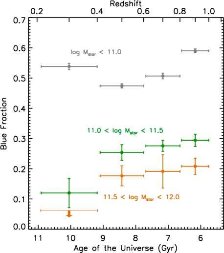
Figure 10: The fraction of the blue population in $<10^{11.0}M_{\odot}$ (grey solid), $10^{11.0-11.5}M_{\odot}$ (green) and $10^{11.5-12.0}M_{\odot}$ (orange) galaxies, respectively, as a function of redshift.

Finally, we comment on the compatibility of the present results with previous studies. There are a number of studies of luminous red galaxies (LRGs) at $z<1$ (e.g., Brown et al., 2007, 2008; Cool et al., 2008) covering up to $\sim$10 deg². Authors consistently suggest that the LRGs show little evolution in number density since $z\sim 1$. However, the mass-to-optical luminosity ratio of galaxies has a significant scatter even for the massive systems, so that galaxies with a certain stellar mass are not quite the equivalent population of galaxies with a certain optical luminosity. This leads to a consequence of most significance for the most massive galaxies: a small portion of the less massive, much more numerous galaxies could contaminate the luminous class of galaxies if their mass-to-luminosity ratios were slightly less than the average, and thus could easily dominate the luminous population. Therefore a subtle (in absolute amplitude) change in the number of most massive galaxies could be drowned out in the measured evolution of the LRGs.

Studies also exist of massive galaxies at $z<1$ with stellar mass measurements based on infrared photometry (e.g., Conselice et al., 2007; Ilbert et al., 2009), although these studies cover a much smaller field of view ($\la$ 1.5 deg²) than ours. In contrast to the present results, they report little evolution in number of the most massive ($>10^{11.5}M_{\odot}$) galaxies. At least part of the discrepancy could be due to small-number statistics and cosmic variance. Actually, while we find $\sim$1000 samples of the most massive galaxies in each redshift bin from our 55.2 deg², the number of samples observed over $\sim$1.5 deg² should be only $\sim$30. We estimate the effects of cosmic variance by dividing our total field into small subfields, each covering $\sim$ 1.5 deg², and measure the number-density fluctuations of massive galaxies among the subfields. As a result, we find that the number densities of the most massive galaxies measured over $\sim$ 1.5 deg² can fluctuate by up to a factor of a few. However, we are not sure whether the above uncertainties alone can account for the discrepancy between the present results and previous ones. The number-density measurements at the steep high end of the galaxy stellar mass function could be heavily affected by contamination arising from less massive galaxies, thus quite accurate analysis is required to unveil the subtle evolution of the most massive galaxies.

In essence, our measurements provide a unique opportunity to investigate the mean properties and evolution of the most massive galaxies, owing to the reliable estimates of photometric redshifts and stellar masses conducted over an unprecedentedly large field of view. What is observationally clear is that we have discovered a substantial deficit of the most massive galaxies out to $z=1$ compared with the local Universe. The analysis of the rest-frame $U-V$ colour distributions indicates that star-formation activity might be responsible for the active build-up of these systems, while it is possible that a so-called dry merger (e.g., Bell et al., 2004; van Dokkum, 2005) is the main driver of the evolution. Actually, some observations suggest that a substantial fraction of massive early-type galaxies go through active evolution in terms of the galaxy structure as well as the star formation since $z\sim$ 1 (e.g., Treu et al., 2005; van der Wel et al., 2008). The present results provide crucial evidence of hierarchical galaxy formation, the missing piece of observation required to chart a course for future theoretical models based on $\Lambda$CDM theory.

6 Summary

We present an analysis of $\sim$60 000 massive galaxies with stellar masses $10^{11}M_{\odot}<M_{\star}<10^{12}M_{\odot}$ in an unprecedentedly large field of view of 55.2 deg². The galaxies are drawn from the UKIDSS Large Area Survey K-band images on the SDSS southern equatorial stripe. We have created deep-stacked $u$, $g$, $r$, $i$ and $z$-band images from the SDSS Supplemental and Supernova Survey image frames, which results in $\sim$90 per cent counterparts of the $K$-band sources in the $g$, $r$, $i$ and $z$ bands. We also exploit the redshift surveys conducted on the SDSS southern equatorial stripe, namely the VIMOS-VLT Deep Survey and the DEEP2 Redshift Survey, in order to obtain accurate photometric redshifts and associated uncertainties for the galaxies. Stellar masses are estimated by comparing the observed broad-band colours with stellar population synthesis models.

In each of the redshift bins $z$ = 0.2–0.4, 0.4–0.6, 0.6–0.8 and 0.8–1.0, we obtain $\sim$10 000 and $\sim$1 000 galaxies with stellar masses $10^{11.0}M_{\odot}<M_{\star}<10^{11.5}M_{\odot}$ and $10^{11.5}M_{\odot}<M_{\star}<10^{12.0}M_{\odot}$, respectively. The galaxies are almost completely detected out to $z=1$, and form by far the largest sample of massive galaxies reaching to the Universe at about half its present age. We find that the most massive ($10^{11.5}M_{\odot}<M_{\star}<10^{12.0}M_{\odot}$) galaxies have experienced rapid growth in number since $z=1$, while the number densities of less massive systems show rather mild evolution. Such a hierarchical trend of evolution is consistent with the predictions of the current semi-analytic galaxy formation model based on $\Lambda$CDM theory. While the majority of the massive galaxies are red-sequence populations, we find that a considerable fraction are blue star-forming galaxies. The blue fraction is less in more massive systems and decreases toward the local Universe, leaving the red, most massive galaxies at low redshifts, which further supports the idea of active bottom-up formation of these populations during $0<z<1$. The present results provide strong evidence that galaxy formation proceeds in a hierarchical way, and place stringent observational constraints on future theoretical models.

References

- Adelman-McCarthy et al. (2008) Adelman-McCarthy J. K., et al., 2008, ApJS, 175, 297
- Bell et al. (2004) Bell E. F., et al., 2004, ApJ, 608, 752
- Bertin & Arnouts (1996) Bertin E., Arnouts S., 1996, A&AS, 117, 393
- Borch et al. (2006) Borch A., et al., 2006, A&A, 453, 869
- Bower, Lucey, & Ellis (1992) Bower R. G., Lucey J. R., Ellis R. S., 1992, MNRAS, 254, 601
- Brown et al. (2007) Brown M. J. I., Dey A., Jannuzi B. T., Brand K., Benson A. J., Brodwin M., Croton D. J., Eisenhardt P. R., 2007, ApJ, 654, 858
- Brown et al. (2008) Brown M. J. I., et al., 2008, ApJ, 682, 937
- Bruzual & Charlot (2003) Bruzual G., Charlot S., 2003, MNRAS, 344, 1000
- Calzetti et al. (2000) Calzetti D., Armus L., Bohlin R. C., Kinney A. L., Koornneef J., Storchi-Bergmann T., 2000, ApJ, 533, 682
- Chabrier (2003) Chabrier G., 2003, PASP, 115, 763
- Cimatti, Daddi, & Renzini (2006) Cimatti A., Daddi E., Renzini A., 2006, A&A, 453, L29
- Cole et al. (2001) Cole S., et al., 2001, MNRAS, 326, 255
- Coleman, Wu, & Weedman (1980) Coleman G. D., Wu C.-C., Weedman D. W., 1980, ApJS, 43, 393
- Conselice et al. (2007) Conselice C. J., et al., 2007, MNRAS, 381, 962
- Cool et al. (2008) Cool R. J., et al., 2008, ApJ, 682, 919
- Cowie et al. (1996) Cowie L. L., Songaila A., Hu E. M., Cohen J. G., 1996, AJ, 112, 839
- Daddi et al. (2000) Daddi E., Cimatti A., Pozzetti L., Hoekstra H., Röttgering H. J. A., Renzini A., Zamorani G., Mannucci F., 2000, A&A, 361, 535
- Davis et al. (2003) Davis M., et al., 2003, SPIE, 4834, 161
- Davé (2008) Davé R., 2008, MNRAS, 385, 147
- De Lucia & Blaizot (2007) De Lucia G., Blaizot J., 2007, MNRAS, 375, 2
- Eddington (1913) Eddington A. S., 1913, MNRAS, 73, 359
- Eggen, Lynden-Bell, & Sandage (1962) Eggen O. J., Lynden-Bell D., Sandage A. R., 1962, ApJ, 136, 748
- Ellis et al. (1997) Ellis R. S., Smail I., Dressler A., Couch W. J., Oemler A. J., Butcher H., Sharples R. M., 1997, ApJ, 483, 582
- Faber et al. (2007) Faber S. M., et al., 2007, ApJ, 665, 265
- Frieman et al. (2008) Frieman J. A., et al., 2008, AJ, 135, 338
- Granato et al. (2004) Granato G. L., De Zotti G., Silva L., Bressan A., Danese L., 2004, ApJ, 600, 580
- Hogg et al. (2003) Hogg D. W., et al., 2003, ApJ, 585, L5
- Huang et al. (2001) Huang J.-S., et al., 2001, A&A, 368, 787
- Ilbert et al. (2006) Ilbert O., et al., 2006, A&A, 457, 841
- Ilbert et al. (2009) Ilbert O., et al., 2009, arXiv, arXiv:0903.0102
- Im et al. (2002) Im M., et al., 2002, ApJ, 571, 136
- Kinney et al. (1996) Kinney A. L., Calzetti D., Bohlin R. C., McQuade K., Storchi-Bergmann T., Schmitt H. R., 1996, ApJ, 467, 38
- Larson (1975) Larson R. B., 1975, MNRAS, 173, 671
- Lawrence et al. (2007) Lawrence A., et al., 2007, MNRAS, 379, 1599
- Le Fèvre et al. (2005) Le Fèvre O., et al., 2005, A&A, 439, 845
- Lemson & Virgo Consortium (2006) Lemson G., the Virgo Consortium, 2006, astro, arXiv:astro-ph/0608019
- Lin et al. (1999) Lin H., Yee H. K. C., Carlberg R. G., Morris S. L., Sawicki M., Patton D. R., Wirth G., Shepherd C. W., 1999, ApJ, 518, 533
- Marchesini et al. (2009) Marchesini D., van Dokkum P. G., Förster Schreiber N. M., Franx M., Labbé I., Wuyts S., 2009, ApJ, 701, 1765
- Matsuoka et al. (2008) Matsuoka Y., et al., 2008, ApJ, 685, 767
- Pei (1992) Pei Y. C., 1992, ApJ, 395, 130
- Salpeter (1955) Salpeter E. E., 1955, ApJ, 121, 161
- Silk & Rees (1998) Silk J., Rees M. J., 1998, A&A, 331, L1
- Skrutskie et al. (2006) Skrutskie M. F., et al., 2006, AJ, 131, 1163
- Somerville et al. (2004) Somerville R. S., Lee K., Ferguson H. C., Gardner J. P., Moustakas L. A., Giavalisco M., 2004, ApJ, 600, L171
- Springel, Di Matteo, & Hernquist (2005) Springel V., Di Matteo T., Hernquist L., 2005, ApJ, 620, L79
- Strateva et al. (2001) Strateva I., et al., 2001, AJ, 122, 1861
- Treu et al. (2005) Treu T., et al., 2005, ApJ, 633, 174
- van der Wel et al. (2008) van der Wel A., Holden B. P., Zirm A. W., Franx M., Rettura A., Illingworth G. D., Ford H. C., 2008, ApJ, 688, 48
- van Dokkum (2005) van Dokkum P. G., 2005, AJ, 130, 2647
- van Dokkum (2008) van Dokkum P. G., 2008, ApJ, 674, 29
- Wake et al. (2006) Wake D. A., et al., 2006, MNRAS, 372, 537
- Warren et al. (2007) Warren S. J., et al., 2007, astro, arXiv:astro-ph/0703037
- White & Rees (1978) White S. D. M., Rees M. J., 1978, MNRAS, 183, 341
- Willmer et al. (2006) Willmer C. N. A., et al., 2006, ApJ, 647, 853
- York et al. (2000) York D. G., et al., 2000, AJ, 120, 1579