Excitonic effects in the optical conductivity of gated graphene

Abstract

We study the effect of electron-electron interactions in the optical conductivity of graphene under applied gate and derive a generalization of Elliott’s formula, commonly used for semiconductors, for the optical intensity. We show that excitonic resonances are responsible for several features of the experimentally measured mid-infrared response of graphene such as the increase of the conductivity beyond the “universal” value above the Fermi blocked regime, the broadening of the absorption at the threshold, and the decrease of the optical conductivity at higher frequencies.

Since its isolation in 2004 nov04 , the demonstration of the presence of electron-electron interactions in the electronic properties of graphene has been elusive rmp . The first clear manifestation of interaction effects comes from the recent measurement of the fractional quantum Hall effect at filling $1/3$ Evafrac ; Kimfrac . To understand the impact of many-body physics in graphene and disentangle it from purely band structure effects it is essential to fully understand graphene’s electronic and transport properties. Furthermore, because Coulomb interactions can be controlled externally by choosing the dielectric constant of the substrate on which graphene is deposited, it is possible to tune the electron-electron interactions in a way that cannot be done in most materials.

An obvious property where to look for correlation effects is the optical response. It is well established that in ordinary semiconductors electron-electron interactions are essential to explain their optical properties Haug2 . For energies below the gap, a particle and a hole created by the excitation process can form a bound state (an exciton), which appears as a well defined peak in the absorption spectra, in the region within the energy gap. For energies above the gap, a renormalization of the band and an enhancement of the optical conductivity is observed and attributed to the Coulomb-mediated scattering between the electron-hole pair. These effects are embodied in the famous Elliott’s formula Haug2 that describes the intensity of optical absorption close to the gap edge. This is true for traditional semiconductors in both three and two dimensions Haug1 . As we are going to show the situation in graphene is, however, quite different.

Firstly, in graphene there is no gap between the lower ($\pi$) and upper ($\pi^{*}$) bands, the effective theory describing graphene’s low energy physics is the massless two-dimensional Dirac equation, and the Coulomb problem in this case has no true bound states, but resonances lin ; coulombpereira ; coulombnovikov ; coulomblevitov . These facts prevent the formation of bound excitons in graphene. On the other hand, exciton resonances can exist and a signature of their presence should be seen in its optical properties kuzmenko ; nair ; mak ; basov ; Crommieopt . Although the system is gapless, the possibility of doping it by using a gate creates an energy interval, of width $2\mu$ ($\mu$ is chemical potential), where light absorption is forbidden due to Pauli’s exclusion principle. In tradicional semiconductors, such a regime is known as the Moss-Burshtein effect. All theoretical investigations of the optical conductivity of gated graphene developed so far evaded the problem of electron-electron interactions and the discussion of excitonic effects nmrPRB06 ; falkovsky ; stauberphonons ; carbotte ; Juan . However, a detailed analysis of the experimental data nair ; basov shows that graphene’s optical conductivity deviates considerably from the non-interacting prediction nair ; basov , even with the inclusion of band structure corrections to the Dirac spectrum staubergeim , disorder, and phonons stauberphonons .

The alluded deviations occur in both neutral and doped graphene, but they are far more evident in the latter case. For neutral graphene, in the visible range of the spectrum at energies around $\sim 3$ eV, the measured percentage of transmitted light, $T$, is smaller than the value $T=1-\pi\alpha\simeq 97.7\%$ ($\alpha$ is the fine structure constant), predicted by the non-interacting theory nair . Band structure effects alone cannot account for the measured deviations staubergeim . In the left inset of Fig. 1 it is shown that calculations based on ab-initio methods can describe, qualitatively, the data (see also Ref. LiLouie, ).

For gated graphene, experiments basov show even more noticeable deviations from the non-interacting picture, which predicts that the optical conductivity of graphene has the form: $\sigma(\omega)=\sigma_{0}\theta(\hbar\omega-2\mu)$, where $\sigma_{0}=\pi e^{2}/(2h)$ is the so-called “universal” AC-conductivity, $\hbar\omega$ is the photon energy, and $\theta(x)$ is the Heaviside step function. The deviations seen in the data are of five different types: (i) finite absorption below $2\mu$, which is due to both inter-band and intra-band elastic and inelastic scattering processes; (ii) broadening of the absorption edge around the energy threshold $2\mu$; (iii) an enhancement of the conductivity above the universal value, $\sigma_{0}$, in the energy range between $2\mu$ and $2\mu+E^{\ast}$, where $E^{\ast}$ is a characteristic energy scale; (iv) a reduction of the conductivity bellow $\sigma_{0}$, at energies above $E^{\ast}$, with the conductivity, as a function of frequency, having a positive curvature; (v) the imaginary part of the conductivity is larger than the value predicted by the non-interacting model for energies $\hbar\omega\gg 2\mu$. Finally, we point out that the optical conductivity curves, for diferent gate voltages basov , collapse on top of each other, when re-plotted as function of $\omega/\mu$, implying that the mechanism causing deviations from the non-interacting approximation must be intrinsic. The analytical microscopic theory we develop in this letter, which includes excitonic effects, accounts for items (ii), (iii), (iv), and (v), and it also partially accounts for item (i), although not completely, since we have not included intra-band scattering in the calculations.

The central result of this work is the calculation of the conductivity of doped graphene, that is, at finite gate voltage, $V_{g}$. The calculation takes into account electron-electron interactions at the exchange level. Its important to stress that the theory given below has no adjustable parameter (except for the use of an effective temperature –see discussion below); the density of impurities is determined by fitting the DC conductivity, that is, it is fixed a priori to the calculations of the optical conductivity. The final result for the latter quantity reads:

$$\sigma=-\frac{ev_{F}}{\pi^{2}}\int d\,\bm{k}\left(\Gamma_{vc,\bm{k}}\chi^{0}_{vc,\bm{k}}d^{x}_{vc,\bm{k}}+\Gamma_{cv,\bm{k}}\chi^{0}_{cv,\bm{k}}d^{x}_{cv,\bm{k}}\right)\,,$$ (1)

where all quantities, to be given below, depend explicitly on $\omega$, and on temperature. In Eq. (1), $e>0$ is the electron charge, $v_{F}$ is the Fermi velocity, $d^{x}_{\lambda\lambda^{\prime},\bm{k}}$ is the matrix element of the dipole operator with $\lambda,\lambda^{\prime}=c,v$ referring to the $\pi^{*}$ ($\pi$) band index, respectively, $\chi^{0}_{\lambda\lambda^{\prime},\bm{k}}$ is the optical susceptibility of graphene in the independent electron approximation, and $\Gamma_{\lambda\lambda^{\prime},\bm{k}}$ is the vertex correction due electron-electron interactions. If we assume $\Gamma_{\lambda\lambda^{\prime},\bm{k}}=1$, Eq. (1) gives the “universal” value for the conductivity of graphene, $\sigma_{0}$. The form of the vertex function reads: $\Gamma_{\lambda\lambda^{\prime},\bm{k}}=[1+s_{vc,\bm{k},1}]^{-1}$, where $s_{vc,\bm{k},1}$ is defined below. This result shows that if $\Gamma_{\lambda\lambda^{\prime},\bm{k}}<1$, its contribution to Eq. (1) acts to reduce $\sigma$ relatively to $\sigma_{0}$. On the other hand, when $\Gamma_{\lambda\lambda^{\prime},\bm{k}}>1$ it contributes to the enhancement of $\sigma$ over $\sigma_{0}$. We show below that the effect of the vertex correction on $\sigma$ depends on $\omega$. The conclusion is then: the importance of electron-electron interactions in graphene can manifest itself in the behavior of $\sigma$ by studying how the data deviates from $\sigma_{0}$. Moreover, the optical conductivity relates to the transmittance by: $T=[(1+\Re\sigma/(2\epsilon_{0}c))^{2}+(\Im\sigma/(2\epsilon_{0}c))^{2}]^{-1}$, where $\epsilon_{0}$ is the vacuum permittivity and $c$ is the speed of light. Our results are summarized in Fig. 1. In the left panel, we depict the real part of the conductivity: the dashed black curve is the non-interacting prediction, considering the effect of disorder; the solid red curve is the prediction taking into account excitonic effects and the same amount of disorder. The right panel refers to the imaginary part of the conductivity. In both panels the experimental data basov is also shown.

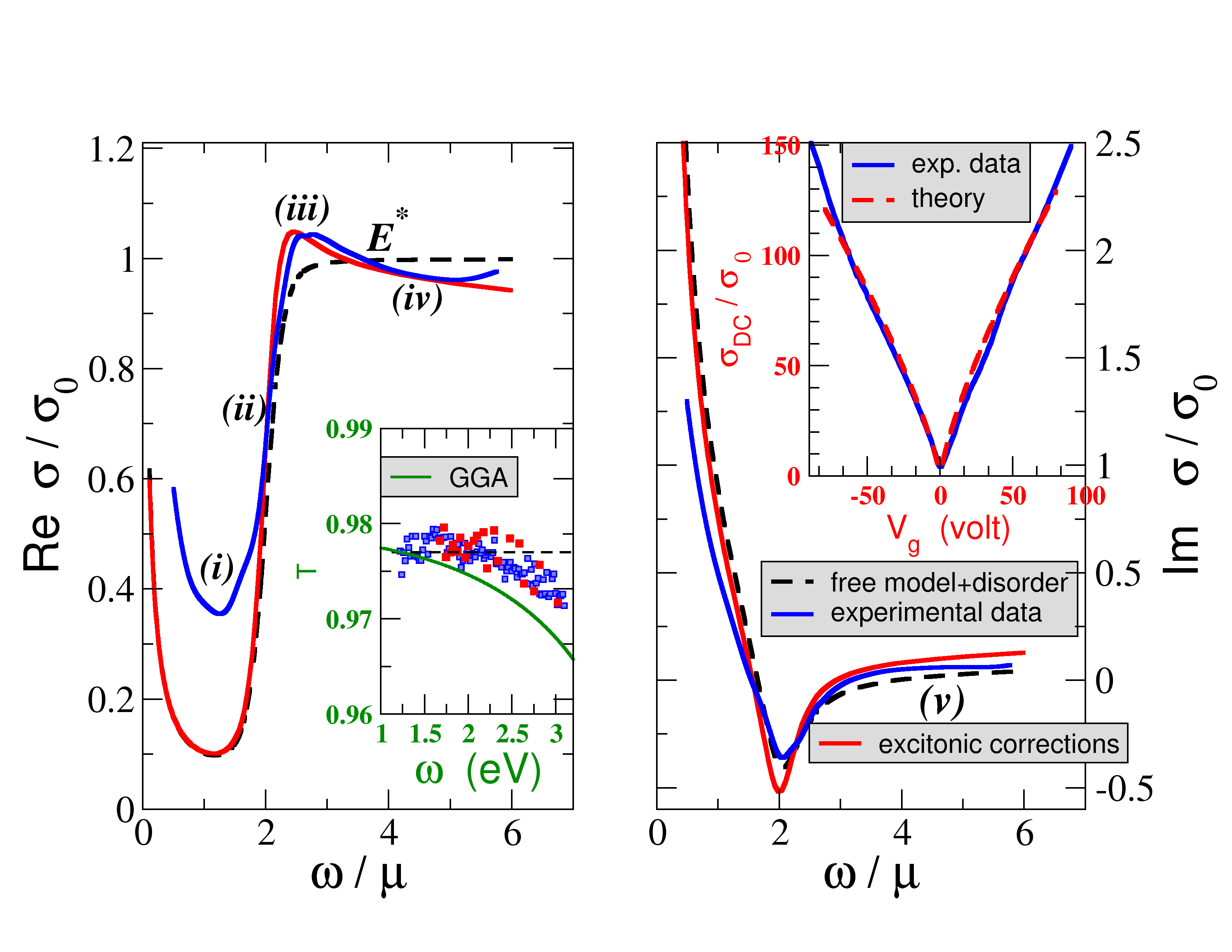
Figure 1: (Color online) Real and imaginary parts of the conductivity. The black dashed line is obtained from the independent electron model with disorder. The solid red line is the model given in the text, which includes excitonic corrections and disorder. The experimental curves, refer to a gate voltage of 28 V, to which corresponds a Fermi energy of $\mu\simeq 0.18$ eV. In the experimentbasov , the chemical potential was given by $\mu=0.03474\sqrt{V}_{g}$ eV. The calculation took an effective temperature of 120 K (see the discussion in point (ii) in the text). In the left inset we give the transmission, $T$, of neutral graphene, as function of $\hbar\omega$, in comparison with the experimental data of Ref. nair, . In the right inset we show the DC conductivity as a function of gate voltage, comparing both the experimental data (blue line) of Ref. basov, and the thoretical fit; the fit fixes the concentration of impurities, to the values of $n_{i}=2\times 10^{11}$ cm^-2, for resonant scatterers, and $n_{i}=1\times 10^{11}$ cm^-2, for charged ones. The determined impurity concentrations are then used in the calculation of the optical conductivity. Therefore, the calculation of the optical conductivity has no fitting parameter. The labels (i), (ii), (iii), (iv), and (v), refer to the five items discussed in the text.

The five items mentioned previously relatively to the data, can easily be observed to be present in the theoretical curve; (i): For $\hbar\omega<2\mu$, there is a finite conductivity, where the non-disordered independent electron model predicts zero absorption. This modification over the naive result is mainly a consequence of disorder, and excitonic effects play no role, as it should be. The discrepancy of about a factor of two between the theory and the data, is to be expected and is a strength of the model, since additional intra-band scattering (the model only includes inter-band scattering) will transfer spectral weight from the Drude peak to this frequency region, enhancing the optical response. (ii): It is clear that disorder and temperature effects combined, account for the broadening of the Fermi step around $2\mu$. As discussed in the context of the optical response of the biased graphene bilayer kuzmenko2 , charge density fluctuations, associated with the random electrostatic potential present at the graphene-SiO₂ interface, smear the Fermi energy, leading to and effective higher temperature than that measured by the finger temperature of the cryostat (in the experimente basov , the temperature of the finger was 54 K); as it is well known, an increase of the temperature broadens Fermi edge staubergeim , as seen in the experiments (we have used the same effective temperature as that used in bilayer graphene, 120 K; this makes sense because the random electrostatic potential alluded above is a property of the substrate). (iii): For $\hbar\omega>2\mu$, an enhancement of the conductivity above $\sigma_{0}$ is seen. This behavior extends to the characteristic energy scale $E^{\ast}$. The energy interval over which $\Re\sigma>\sigma_{0}$ is about the same in the theory and in the data. Finally, we should stress that the results of Fig. 1 were obtained from an approximate analytical solution to the vertex functions. Corrections to this approximation may also account for the small differences between the data and the theoretical curves. (iv): For $\hbar\omega>E^{\ast}$, the conductivity goes below $\sigma_{0}$, over a large energy range, presenting a positive curvature. Exactly the same behavior is seen in our calculations, with the decrease of the conductivity below $\sigma_{0}$ having about the same numerical value. (v): The imaginary part of the conductivity, $\Im{\sigma}$, is larger, for energies above $\sim 3\mu$, than that predicted by the non-interacting model with disorder and fits well the data. In conclusion, Eq. (1) does explain all features, (ii)-(iv), of the experimental data basov , making clear that electron-electron interaction effects are manifestly present in the optical conductivity of gated graphene for $\hbar\omega\geq 2\mu$. Finally, we must note in passing that we have chosen to fit a set of data where no renormalization of the Fermi velocity was measured basov , since our model does not include the renormalization of the electronic velocity For all data sets such that $V_{g}\geq 28$ V, no Fermi velocity renormalization was measured; we have chosen the first of this class of sets, namely that for which $V_{g}=28$ V.

Before discussing the calculation of the electron-electron corrections to the optical conductivity, it is instructive to show that the formalism based on the polarization concept gives the well known result for the “universal” conductivity of graphene. As it will be clear, this formalism bypasses the calculation of the Kubo formula stauberphonons ; carbotte . The low-energy Hamiltonian of graphene, with a vector potential, $\bm{A}(\bm{r},t)$, reads: $H=v_{F}\bm{\sigma}\cdot[\bm{p}+e\bm{A}(\bm{r},t)]=H_{0}+H_{I}\,.$ Assuming an electric field of the form $\bm{E}(t)=E_{0}{\hat{\bf x}}e^{-i\omega t}$, the interaction of the electrons with light is given by $H_{I}=ev_{F}A_{0}\sigma_{x}e^{-i\omega t}=ev_{F}\sigma_{x}A_{0}(t)$, with $A_{0}=-iE_{0}/\omega$. The polarization along the $x-$direction is:

$$P_{x}(t)=\sum_{\sigma}\int d\,\bm{r}\langle\hat{\psi}^{\dagger}_{\sigma}(\bm{r},t)d_{x}\hat{\psi}_{\sigma}(\bm{r},t)\rangle\,,$$ (2)

where $d_{x}$ is the dipole operator, $d_{x}=-v_{F}e\sigma_{x}$, and $\hat{\psi}_{\sigma}(\bm{r},t)$ is the field operator:

$$\hat{\psi}_{\sigma}(\bm{r},t)=\sum_{\bm{k},\lambda}a_{\lambda,\bm{k},\sigma}(t)\psi_{\lambda,\bm{k}}(\bm{r})\,,$$ (3)

with $\psi_{\lambda,\bm{k}}(\bm{r})$ the eigenfunctions of $H_{0}$ rmp , $a_{\lambda,\bm{k},\sigma}$ the destruction operator of an electron in band $\lambda$, with momentum $\bm{k}=(k_{x},k_{y})$, and spin projection $\sigma$ ($\lambda=1$ for $\lambda=c$ and $\lambda=-1$ for $\lambda=v$). The matrix element of the dipole operator reads: $d_{\lambda,\lambda^{\prime},\bm{k}}^{x}=(\lambda^{\prime}e^{i\theta(\bm{k})}+\lambda e^{-i\theta(\bm{k})})/2$, with $\tan\theta(\bm{k})=k_{y}/k_{x}$. Then, the final expression for the polarization (per unit time) $P_{x}(t)$ is, in second quantized form, given by:

$$P_{x}(t)=-Ev_{F}\sum_{\sigma,\lambda,\lambda^{\prime}}\sum_{\bm{k}}\langle a^{\dagger}_{\lambda,\bm{k},\sigma}(t)a_{\lambda^{\prime},\bm{k},\sigma}(t)\rangle d_{\lambda,\lambda^{\prime},\bm{k}}^{x}\,,$$ (4)

and $H_{I}$ reads:
$H_{I}=v_{F}eA(t)\sum_{\sigma,\lambda,\lambda^{\prime}}\sum_{\bm{k}}a^{\dagger}_{\lambda,\bm{k},\sigma}a_{\lambda^{\prime},\bm{k},\sigma}d_{\lambda,\lambda^{\prime},\bm{k}}^{x}\,.$

We introduce the dipolar operator $\hat{P}_{vc,\bm{k}}=a^{\dagger}_{v,\bm{k}}a_{c,\bm{k}}$, and seek the solution of its equation of motion, $-i\hbar\partial\hat{P}_{vc,\bm{k}}/\partial t=[H,\hat{P}_{vc,\bm{k}}]$. The procedure is simple, and gives the following result for the thermal average of the operator $\hat{P}_{vc,\bm{k}}$:

$$\langle\hat{P}_{vc,\bm{k}}\rangle=v_{F}eA_{0}d^{x}_{cv,\bm{k}}\frac{n_{F}(E_{c,\bm{k}})-n_{F}(E_{v,\bm{k}})}{-\omega\hbar-i\Gamma-E_{v,\bm{k}}+E_{c,\bm{k}}}\,,$$ (5)

where $n_{F}(x)$ is the Fermi function, $E_{c/v,\bm{k}}=\pm v_{F}\hbar k$, and $\Gamma(\omega)$ is the level broadening (a similar equation follows for $\langle\hat{P}_{cv,\bm{k}}\rangle$). We note that the broadening $\Gamma(\omega)$ is not a constant, but follows a well prescribed model, where the scattering is dominated by resonant and charged scatterers stauberBZ ; coulombnovikov : $\Gamma(\omega)=n^{(\rm rs)}_{i}v_{F}\hbar\sigma^{(\rm rs)}_{T}(\omega)+n^{(\rm ch)}_{i}v_{F}\hbar\sigma^{(\rm ch)}_{T}(\omega)$, where $n_{i}^{(\rm rs/ch)}$ is the concentration of impurities and $\sigma_{T}^{(rs/ch)}(\omega)$ is the exact transport cross section, for each type of scatterers. Once $\langle\hat{P}_{\lambda\lambda^{\prime},\bm{k}}\rangle$ is known, the calculation of the polarization per unit area, $p_{x}=P_{x}(\omega)/A$, follows from Eq. (4) as:

$$p_{x}=-i\frac{2e^{2}v_{F}^{2}E_{0}}{\omega A}\sum_{\bm{k},\lambda\neq\lambda^{\prime}}s(\bm{k})\frac{n_{F}(E_{\lambda,\bm{k}})-n_{F}(E_{\lambda^{\prime},\bm{k}})}{\omega\hbar-E_{\lambda,\bm{k}}+E_{\lambda^{\prime},\bm{k}}+i\Gamma}\,,$$ (6)

where $s(\bm{k})=\sin^{2}[\theta(\bm{k})]$, and the optical conductivity is simply given by $\sigma=p_{x}/E_{0}$. Equation (6) for the conductivity of graphene is the same one obtained by computing the Kubo formula from the current-current correlation function staubergeim . If we consider, as a simple example, the limiting case where $\Gamma\rightarrow 0$, $\mu=0$, and zero temperature, Eq. (6) gives $p_{x}/E_{0}=\pi e^{2}/(2h)=\sigma_{0}$.

We can extend the formalism above to the case where electron-electron interactions are considered, and use it to derive the central result of this work, Eq. (1). The formalism we present below, gives results equivalent to the solution of the Bethe-Salpeter equation, but following a more straightforward path. Electron-electron interactions in graphene are described by the Hamiltonian:

$$H_{e-e}=\frac{1}{2}\int d\,\bm{r}d\,\bm{r}^{\prime}\hat{\psi}^{\dagger}(\bm{r})\psi^{\dagger}(\bm{r}^{\prime})V(\bm{r}-\bm{r}^{\prime})\psi(\bm{r}^{\prime})\psi(\bm{r})\,,$$ (7)

where $V(\bm{r})$ is the Coulomb potential. Since we are studying the conductivity of gated graphene, the Coulomb potential is screened, and at the level of the Thomas-Fermi approximation (corresponding to the static RPA limit) the Fourier transform of the Coulomb potential reads: $\varphi_{\rm 2D}(\bm{q})=e^{2}[2\epsilon_{0}(q+q_{\rm TF})]^{-1}\,,$ with the Thomas-Fermi momentum, $q_{\rm TF}$, defined as $q_{\rm TF}=4\alpha_{g}\sqrt{\pi n_{e}}$, where $n_{e}$ is the electron density per unit area and $\alpha_{g}=e^{2}/(4\pi\epsilon_{0}v_{F}\hbar)$ (for graphene on top of SiO₂ we replace $\epsilon_{0}$ by $\epsilon_{0}\epsilon_{\rm SiO_{2}}$ and $e^{2}/(4\epsilon_{0}\epsilon_{\rm SiO_{2}}v_{F}\pi\hbar)\approx 1/2$; in our calculations we used $\alpha_{g}=0.4$). Introducing the field operators (3) in Eq. (7), the electron-electron interaction in the momentum representation reads:

$$H_{e-e} = \frac{1}{8A}\sum_{\{\lambda_{i}\}}\sum_{\bm{k},\bm{k}^{\prime},\bm{q}}\sum_{\sigma,\sigma^{\prime}}\varphi_{\rm 2D}(\bm{q})a^{\dagger}_{\lambda_{1},\bm{k}+\bm{q},\sigma}a^{\dagger}_{\lambda_{2},\bm{k}^{\prime}-\bm{q},\sigma^{\prime}}\times$$ (8)

$$a_{\lambda_{3},\bm{k}^{\prime},\sigma^{\prime}}a_{\lambda_{4},\bm{k},\sigma}f(\bm{k}^{\prime},-\bm{q})_{\lambda_{2},\lambda_{3}}f(\bm{k},\bm{q})_{\lambda_{1},\lambda_{4}}\,,$$

where $f(\bm{k},\bm{q})_{\lambda_{a},\lambda_{b}}=(1+\lambda_{a}\lambda_{b}e^{-i[\theta(\bm{k}+\bm{q})-\theta(\bm{k})]})\,.$ As before, we seek the equation of motion for the operator $\hat{P}_{vc,\bm{k}}=a^{\dagger}_{v,\bm{k}}a_{c,\bm{k}}$, but now in the presence of electron-electron interactions. To that end, we need to compute the commutator of $\hat{P}_{vc,\bm{k}}$ with $H_{e-e}$, in addition to the one we have already determined for the non-interacting theory. The evaluation of $\langle[H_{e-e},\hat{P}_{vc,\bm{k}}]\rangle$, after making the usual Hartree-Fock decoupling the quartic terms, gives:

$$\langle[H_{e-e},\hat{P}_{vc,\bm{k}}]\rangle\!\! = \!\!C^{\rm exch.}\!+\!C^{\rm excit.}\!+\!C^{\rm dens.}+C^{\rm n-l}\,,$$ (9)

where the several terms have the following physical interpretation: $C^{\rm exch.}$ is the exchange correction to the bare bands; $C^{\rm excit.}$ are the excitonic contributions, coming from the Coulomb interaction among the electron-hole pair formed by the absorption of light; $C^{\rm dens.}$ is the interaction of the electrons and holes in the bands with the electron gas formed by the gating; and $C^{\rm n-l}$ are non-linear terms in the field intensity, $E_{0}$, due to the interaction of the average of the operator $\hat{P}_{vc,\bm{k}}$ with itself and with the average of the operator $\hat{P}_{cv,\bm{k}}$ (see also Ref. Mishchenko, ).

Let us consider the calculation of the vertex corrections, $\Gamma_{\lambda\lambda^{\prime},\bm{k}}$, entering in Eq. (1). We ignore the non-linear corrections included in the commutator (9). The term $C^{\rm density}$ can be shown to give a zero contribution to the polarization of the material. From the commutator (9), the full equation of motion for the operator $\hat{P}_{vc,\bm{k}}$ gives:

$$(-\omega\hbar-E_{v,\bm{k}}+E_{c,\bm{k}})\langle\hat{P}_{vc,\bm{k}}\rangle=E_{0}\frac{v_{F}e}{i\omega}d^{x}_{cv,\bm{k}}\delta n_{F,\bm{k}}$$ (10)

$$+ \delta n_{F,\bm{k}}\frac{1}{2A}\sum_{\bm{q},\sigma}\varphi_{\rm 2D}(\bm{q})\langle\hat{P}_{vc,\bm{k}-\bm{q}}\rangle F_{+,+}(\bm{k},\bm{q})$$

$$+ \delta n_{F,\bm{k}}\frac{1}{2A}\sum_{\bm{q},\sigma}\varphi_{\rm 2D}(\bm{q})\langle\hat{P}_{cv,\bm{k}-\bm{q}}\rangle F_{-,-}(\bm{k},\bm{q})\,,$$

with $\delta n_{F,\bm{k}}=[n_{F}(E_{c,\bm{k}})-n_{F}(E_{v,\bm{k}})]$ and $F_{\lambda,\lambda}(\bm{k},\bm{q})=1+\lambda\cos[\theta(\bm{k})-\theta(\bm{k}-\bm{q})]$. Eq. (10) and the equivalent one for $\langle\hat{P}_{cv,\bm{k}}\rangle$, obtained from Eq. (10) by interchanging the labels $c$ and $v$, form a set of two coupled integral equations. The approximate solution of this set of equation is obtained as follows: since we are interested in the linear response, we write $P_{vc,\bm{k}}=E_{0}\chi_{vc,\bm{k}}$. Additionally, the function $\chi_{vc,\bm{k}}$ is written in terms of the $\chi^{0}_{vc,\bm{k}}$ (which represents $\chi_{vc,\bm{k}}$ in the absence of electron-electron interactions) as $\chi_{vc,\bm{k}}=\Gamma_{vc,\bm{k}}\chi^{0}_{vc,\bm{k}}$, where $\Gamma_{vc,\bm{k}}$ is the vertex function. After these operations, a set of coupled integral equations for the vertex functions is obtained from Eq. (10), which is then solved by the method of Padé approximants Haug1 . For simplicity, we have only considered the leading approximant. The method of solution described here is equivalent to summing an infinite sub-set of Feynman diagrams, and it gives the analytical solution for the vertex in the form $\Gamma_{\lambda\lambda^{\prime},\bm{k}}\approx[1+s_{vc,\bm{k},1}]^{-1}$ with the $s_{\lambda\lambda^{\prime},\bm{k},1}$ defined as

$$s_{\lambda\lambda^{\prime},\bm{k},1}\!\! = \!\!-\!\frac{\omega}{v_{F}e\sin\theta_{\bm{k}}}\Theta_{\lambda\lambda^{\prime},\bm{k}}^{+}\!\!-\!\!\frac{\omega}{v_{F}e\sin\theta_{\bm{k}}}\Theta_{\lambda^{\prime}\lambda,\bm{k}}^{-}\,.$$ (11)

where,

$$\Theta_{\lambda\lambda^{\prime},\bm{k}}^{\pm}\!\!=\!\!\frac{1}{2\pi^{2}}\int_{0}^{2\pi}\!\!d\theta_{\bm{q}}\int_{0}^{q_{c}}\!\!qdq\varphi_{\rm 2D}(\bm{q}-\bm{k})\chi^{0}_{\lambda\lambda^{\prime},\bm{q}}[1\pm\cos(\theta_{\bm{k}}\!-\!\theta_{\bm{q}})]\,.$$ (12)

This procedure for determining the vertex function is equivalent to the RPA solution of the Bethe-Salpeter equation hanke ; we believe, however, that our method is more straightforward. Equations (11) and (12) can be used to determine the vertex function in closed form. The bare susceptibility, $\chi^{0}_{\lambda\lambda^{\prime},\bm{k}}$, is given by

$$\chi^{0}_{\lambda\lambda^{\prime},\bm{k}}\!=\!-\sin\theta_{\bm{k}}\frac{ev_{F}}{\omega}\!\left(\!\frac{n_{F}(E_{\lambda,\bm{k}})\!-\!n_{F}(E_{\lambda^{\prime},\bm{k}})}{\hbar\omega\!-\!E_{\lambda^{\prime},\bm{k}}\!+\!E_{\lambda,\bm{k}}\!+\!i\Gamma}\!+\!\lambda^{\prime}\frac{\theta(k)}{2v_{F}\hbar k}\right)\,,$$ (13)

where $\theta(k)$ is the Heaviside step function. Unfortunately the integrals cannot be evaluated analytically but can easily be obtained by numerical integration.

In summary, we have developed a general formalism for taking into account excitonic effects in graphene. These effects were computed taking the lowest Padé approximant, but higher order ones can be easily introduced and may improove the fit of the data. Additional many-body effects, such as inelastic phonon scattering can also be easily included, which makes the formalism a powerful one to study the combined effects of disorder, electronic correlations, and phonon scattering in graphene’s optical spectrum. Extending the formalism to visible range of the spectrum is also feasible, by computing the eigenproblem of the free theory including trigonal warping effects. Finally, we have showed that our formalism solves discrepancies between the data basov and the theoretical results provided by the independent electron picture.

AHCN acknowledges DOE grant DE-FG02-08ER46512 and ONR grant MURI N00014-09-1-1063. NMRP acknowledges the FCT grant PTDC/FIS/111524/2009, and T. Stauber and M. Vasilevskiy for comments at an earlier stage of the manuscript.

References

- (1) K. S. Novoselov et al., Science 306, 666 (2004)
- (2) A. H. Castro Neto et al., Rev. Mod. Phys. 81, 109 (2009)
- (3) Xu Du et al., Nature 462, 192 (2009)
- (4) Kirill I. Bolotin et al., Nature 462, 196 (2009)
- (5) H. Haug and S. W. Koch, Phys. Rev. A 39, 1887 (1989)
- (6) C. Ell et al., J. Opt. Soc. Am. B 6, 2006 (1989)
- (7) Q.-G. Lin, Phys. Lett. A 26, 17 (1999)
- (8) Vitor M. Pereira et al., Phys. Rev. Lett. 99, 166802 (2007)
- (9) D. S. Novikov, Phys. Rev. B 76, 245435 (2007)
- (10) A. V. Shytov et al., Phys. Rev. Lett. 99, 236801 (2007)
- (11) A. B. Kuzmenko et al., Phys. Rev. Lett. 100, 117401 (2008)
- (12) R. R. Nair et al. , Science 320, 1308 (2008)
- (13) Kin Fai Mak et al., Phys. Rev. Lett. 101, 196405 (2008)
- (14) Z. Q. Li et al., Nature Phys. 4, 532 (2008)
- (15) Feng Wang et al., Science 320, 206 (2008)
- (16) N. M. R. Peres et al., Phys. Rev. B 73, 125411 (2006)
- (17) L. A. Falkovsky and S. S. Pershoguba, Phys. Rev. B 76, 153410 (2007)
- (18) T. Stauber et al., Phys. Rev. B 78, 085418 (2008)
- (19) V. P. Gusynin et al., New J. Phys. 11, 095013 (2009)
- (20) Adolfo G. Grushin et al., Phys. Rev. B 80, 155417 (2009)
- (21) T. Stauber et al., Phys. Rev. B 78, 085432 (2008)
- (22) Li Yang et al., Phys. Rev. Lett. 103, 186802 (2009)
- (23) A. B. Kuzmenko et al., Phys. Rev. B 80, 165406 (2009)
- (24) T. Stauber et al., Phys. Rev. B 76, 205423 (2007)
- (25) E. G. Mishchenko, Phys. Rev. Lett. 103, 246802 (2009)
- (26) W. Hanke et al., Phys. Rev. B 21, 4656 (1980)