The Dirac operator spectrum: a perturbative approach

Abstract:

By computing the Dirac operator spectrum by means of Numerical Stochastic Perturbation Theory, we aim at throwing some light on the widely accepted picture for the mechanism which is behind the Bank-Casher relation. The latter relates the chiral condensate to an accumulation of eigenvalues in the low end of the spectrum. This can be in turn ascribed to the usual mechanism of repulsion among eigenvalues which is typical of quantum interactions. First results appear to confirm that NSPT can indeed enable us to inspect a huge reshuffling of eigenvalues due to quantum repulsion.

1 Introduction

Chiral symmetry breaking is one the key feature of QCD. There is a very intuitive way of stating the physics of this phenomenon: a small quark mass leads to a macroscopic realignment of the QCD vacuum (this is a strict quotation from [1]). Since the QCD partition function reads

$$Z=\langle\prod_{f}\det({\cal D}+m_{f})\rangle=\langle\prod_{f}\prod_{n}(i\lambda_{n}+m_{f})\rangle$$ (1)

in order for this to be possible there must be an accumulation of Dirac operator eigenvalues near zero (otherwise the effect of a small quark mass would be overwhelmed by much larger eigenvalues). This message is actually encoded in the Banks Casher relation [2]

$$\langle\bar{\psi}\psi\rangle=\frac{\pi\rho(0)}{V}$$ (2)

relating the chiral condensate (the order parameter of the transition associated to spontaneous symmetry breaking) to the density of eigenvalues of the Dirac operator spectrum

$$\rho(\lambda)=\langle\sum_{n}\delta(\lambda-\lambda_{n})\rangle.$$ (3)

Altought not a natural observable in Field Theory, the Dirac operator spectrum has in force of (2) become a natural probe for the chiral transition. Recent work [3] has investigated the field theoretic status of spectral observables, in particular with respect to their renormalization properties. From a numerically point of view, it should be pointed out that Lattice QCD can quite naturally compute (3), once a lattice regularization of the Dirac operator is given.

2 The Dirac spectrum and Perturbation Theory

Since the free Dirac operator has a vanishing eigenvalues density near zero, one is lead to the conclusion that the small eigenvalues are due to gauge interactions. There is actually a natural candidate: any quantum interaction produces a repulsion among the eigenvalues. With this respect Perturbation Theory is in a tantalizing situation:

• on one side, it sits (deep) in the chirally restored regime, while one looks for an effect which lives at its border;

• on the other side, it gives a unique opportunity to follow the fate of eigenvalues in their mutual repulsion.

We want to emphasize that our work is still at a very preliminary stage. In particular, we do not want to address here the subtleties which arise in properly defining a perturbative expansion of (3). We will discuss a quick and dirty procedure in which we first compute the perturbative corrections to the free spectrum eigenvalues

$$\lambda_{n}=\lambda_{n}^{(0)}+\beta^{-1/2}\lambda_{n}^{(1)}+\beta^{-1}\lambda_{n}^{(2)}+\ldots$$

and then resum the expansion at given values of the coupling $\beta$. Given these summations, we can proceed to compute a density of eigenvalues much the same as in non-perturbative computations of the spectrum.

3 The Dirac Spectrum in NSPT

Numerical Stochastic Perturbation Theory [4] relies on an expansion of the solution of Langevin equation. In the case of LGT

$$U_{x\mu}(\tau;\eta)\rightarrow 1+\sum_{k=1}\beta^{-k/2}U^{(k)}_{x\mu}(\tau;\eta).$$ (4)

$\tau$ is the stochastic time of Langevin evolution, with gaussian noise $\eta$. For asymptotic values of the stochastic time, $\eta$-averages $\langle\ldots\rangle_{\eta}$ of observables converge order by order to quantum field theory averages $\langle\ldots\rangle_{QFT}$.

Plugging (4) into the Dirac operator turns the computation of (3) into the typical eigenvalue/eigenvector problem in PT

$$M=M_{0}+N=M_{0}+\sum_{i}g^{i}N_{i}\;\;\;\;\;\;\;\;\;M\,|\alpha\rangle=\epsilon\,|\alpha\rangle$$ (5)

which has to be solved by

$$\epsilon=\epsilon_{0}+g\,\epsilon_{1}+g^{2}\,\epsilon_{2}+\ldots\;\;\;|\alpha\rangle=|\alpha_{0}\rangle+g\,|\alpha_{1}\rangle+g^{2}\,|\alpha_{2}\rangle+\ldots$$ (6)

Due to the (huge) degeneracy of the free field solution, for every eigenvalue we need to explicitly separate components inside and outside the starting (degenerate) eigenspace, i.e.

$$|\alpha\rangle=|\alpha_{0}\rangle+P^{\prime}_{in}|\alpha\rangle+P_{out}|\alpha\rangle.$$ (7)

In the previous formula $|\alpha_{0}\rangle$ is the direction in the free (degenerate) eigenspace singled out as the zeroth order of the solution; $P^{\prime}_{in}$ is the projector onto the component of the free eigenspace which is orthogonal to $|\alpha_{0}\rangle$; $P_{out}$ projects instead outside the free eigenspace. We finally get the iterative solution

$$\epsilon_{n} = \sum_{k=0}^{n}\,\langle\alpha_{0}|N_{n-k}|\alpha_{k}\rangle$$ (8)

$$P_{out}|\alpha\rangle = (\epsilon-M_{0}-P_{out}N)^{-1}\left(\,P_{out}N|\alpha_{0}\rangle+P_{out}NP^{\prime}_{in}|\alpha\rangle\,\right)$$

$$P^{\prime}_{in}|\alpha\rangle = \;(\epsilon-\epsilon_{0}-P^{\prime}_{in}N)^{-1}\;\;\left(\,P^{\prime}_{in}N|\alpha_{0}\rangle+P^{\prime}_{in}NP_{out}|\alpha\rangle\,\right).$$

This is the (closed) solution only provided degeneracy is lifted at first order. Should this not be the case, the formalism should be generalized by introducing a new projector for each level of degeneracy still present (the solution is nevertheless closed also in such a situation, which actually occurs in our computations).

In standard non-perturbative LGT computations of the Dirac operator spectrum one gets distributions of eigenvalues by generating configurations and computing the spectrum on each of them. The density of eigenvalues is then simply obtained by plain histograms of the results. We stress once again that at this stage of our work we will adhere to the naive recipe of first computing the eigenvlaues in PT, then summing the expansions at given values of the coupling and finally constructing histograms much the same way as in the non-perturbative case.

4 Results

In figure (1) we plot examples of our results: we collect all the measurements for first (trivial) and second (one loop) order corrections to free field results for the second lowest lying eigenspace on a $6^{4}$ lattice. We stress that this eigenspace is degenerate (the dimension of this eigenspace is $144$), but on top of this degeneracy the histograms entail the multeplicity which comes from the number of measurements.

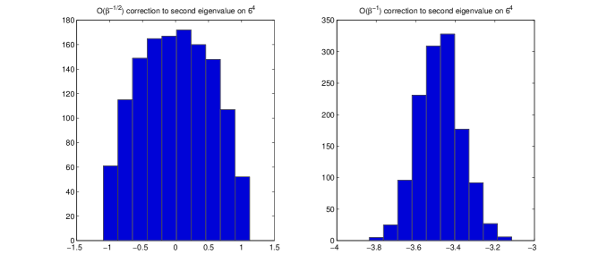
Figure 1: First (trivial) and second (one loop) corrections to the second (lowest lying) free field eigenvalue on a $6^{4}$ lattice (overall distributions of the measures).

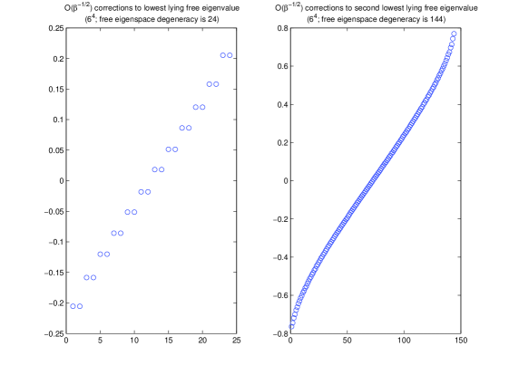
Figure 2: First (trivial) corrections to the first (lowest lying) and second free field eigenvalue on a $6^{4}$ lattice (averages over Langevin histories). Free eigenspace degeneracies are 24 (left) and 144 (right).

Figure (2) displays data once the average over all the measurements has been taken. In this case we plot first order corrections (as one expects, they average to zero) for lowest lying and second lowest lying eigenvalues. There are issues which are worth stressing. First of all, one can ispect degeneracies which are not lifted. Second, the distributions of corrections in the two eigenspaces differ quite a lot.

Figure (3) displays another interesting feature. In this case we plot a third order correction, which enlights how higher orders display long tails. One probably needs to carefully assess when the free field degeneracy is actually lifted, as it is clear from the impact of denominators in (8).

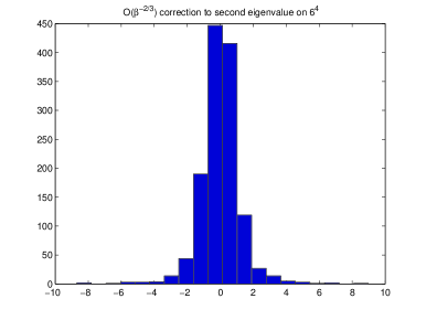
Figure 3: Third correction to the second free field eigenvalue on a $6^{4}$ lattice: while it is centered in zero (as expected), it displays long tails.

With this respect we point out that one can always check the accuracy of the computation by considering quantities like

$$\;\;\;\;\;\;\;\;\langle\mbox{Tr}(D^{\dagger}D)^{k}\rangle=\ldots\;\;\;\;\;\;\;\;\langle\mbox{Tr}(D^{\dagger}D)^{-k}\rangle=\ldots$$

They can be both computed directly and reconstructed from the eigenvalues distribution, eventually validating the latter.

We can now go back to our quick and dirty procedure to inspect the impact of the perturbative corrections. Basically, we can sum the contributions at any given value of the coupling and try to follow the resulting distribution of eigenvalues as the gauge intercation comes into play. We plot in figure (4) what we get at one loop.

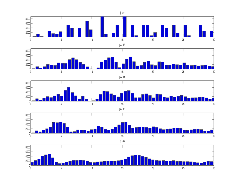
Figure 4: The evoultion of the eigenvalues density: from free field limit ($\beta=\infty$) to the intercating case (at different values of the coupling $\beta$).

Figure (4) is something like a sequence of pictures taken while the interaction is switched on. One starts at zero coupling, where the key feature of the free field is on display: bins are centered where free field eigenvalues sit, and bins heigth simply entails the degeneracy of the various eigenspaces. Notice anyway that at this resolution some bins actually results from the contribution of two free field eigenvalues sitting very close to each other. While the interaction is switched on (i.e. the value of the inverse coupling $\beta$ decreases) the bins spread and overlap and eventually a non-zero density near zero is generated. A natural question arises: where do eigenvalues moving to zero come from? One should remember the point we made on repulsion among eigenvalues. Figure (5) displays an example of how this takes place: we plot the contribution to $\rho$ coming from two eigenvalues starting very close to each other in free field.

It is worth better assessing the impact of the repulsion among the couple of free eigenvalues we have just looked at. It actually turns out that they give a substantial contribution to the rearrangement of the eigenvalues density: one can recognize their splitting on the right of figure (6).

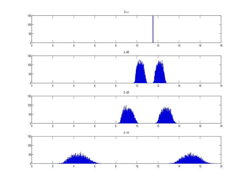
Figure 5: Following the repulsion of two eigenvalues on $6^{4}$. They start very close in free field limit and then strongly repel each other.

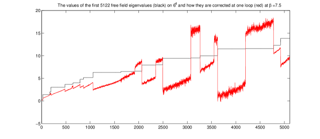
Figure 6: The first 5122 free eigenvalues on a $6^{4}$ lattice (black line): the lenghts of each segment is the degeneracy in free field. Red curve displays how they move at one loop at $\beta=7.5$.

Black line in figure (6) is nothing but another way of plotting the first row of figure (4): we plot the first 5122 free eigenvalues and the lenght of each plateaux is just the degeneracy of each free field eigenspace. The superimposed red line shows the summation (at first loop) of the perturbative series for these eigenvalues at $\beta=7.5$.

Some caveats are of course in order:

• Is this a finite-volume effect? At the moment we have actually got the same qualitative picture at any (still moderate) size we studied.

• Is this a finite $a$ effect? Testing this is more difficult.

• One should carefully take care of the order of limits which is in place in the Banks Casher relation.

A few following steps are on their way: we will repeat the computation in the background of different $Z(3)$ vacua and to try to reconstruct the Polyakov loop from the spectral decomposition of the Dirac operator (this is in the spirit of recent works by Gattringer [5]).

5 Conclusions

Even though at a very preliminary stage, we showed some results of a perturbative computation of the Dirac operator spectrum by means of NSPT. Our results quantitatively support the picture of the repulsion among eigenvalues being responsible for the rearrangement of eigenvalues, ultimately giving rise to Banks Casher.

Some developments of this work are expected to follow these preliminary results.

• We have to carefully assess the huge tails of higher order distributions. One hint is that this asks for some regulator in highly degenerate free field eigenspaces.

• We will move to computations in the background of different $Z(3)$ vacua.

• Having at hand full spectra could in principle enable the computation of a variety of quantities.

References

- [1] J.J.M. Verbaarschot and T. Wettig, Ann. Rev. Nucl. Part. Sci. (2000) 343.
- [2] T. Banks and A. Casher, Nucl. Phys. B169 (1980) 103.
- [3] L. Giusti and M. Luescher, JHEP 0903 (2009) 013.
- [4] F. Di Renzo and L. Scorzato, JHEP 0410 (2004) 073.
- [5] C. Gattringer, Phys. Rev. Lett 97 (2006) 032003.