High loop renormalization constants for Wilson fermions/Symanzik improved gauge action

Abstract:

We present the current status of our computation of quark bilinear renormalization constants for Wilson fermions and Symanzik improved gauge action. Computations are performed in Numerical Stochastic Perturbation Theory. Volumes range from $10^{4}$ to $32^{4}$.
Renormalization conditions are those of the RI’-MOM scheme, imposed at different values of the physical scale. Having measurements available at several momenta, irrelevant effects are taken into account by means of hypercubic symmetric Taylor expansions. Finite volumes effects are assessed repeating the computations at different lattice sizes. In this way we can extrapolate our results to the continuum limit, in infinite volume.

1 Motivations

For a long time, lattice perturbation theory was the only available tool for the computation of Lattice QCD Renormalization Constants (RC’s). Since the introduction of methods that allow the non perturbative computation of the RC’s for generic composite operators [1][2], these techniques are preferred. Nevertheless there is no theoretical obstacle to the perturbative computation of either finite or logarithmically divergent RC’s. In principle, Lattice Perturbation Theory (LPT) provides the connection between lattice simulations and continuum perturbative QCD, that works only at high energy. The main difficulties of LPT are actually practical. First of all, LPT requires much more effort than in the continuum. Because of this, a lot of perturbative results are known only at one loop. Second, LPT series present bad convergence proprieties, so that we should emphasize that a fortiori one loop computations cannot give the correct results. A good example is provided by the computation of the quark mass renormalization constant: there appear to be discrepancies in between determinations coming from perturbative and non-perturbative techniques [3]. The very point is that as long as a comparison is made taking into account one loop, it is virtually impossible to assess the systematics of both results.
In order to obtain higher orders in PT expansions, one can make use of Numerical Stochastic Perturbation Theory (NSPT) [4], a numerical implementation of Stochastic PT [5]. Renormalization constants can be computed in NSPT at 3 (or even 4) loops, as it has been done in the case of Wilson fermions with non-improved gauge actions [6]. A nice aspect is that one can work in the massless limit, where RC’s are often defined, and no chiral extrapolation is needed. We will discuss how one can assess to finite $a$ effects by means of hypercubic Taylor expansion. Moreover, finite volume effects can be corrected by repeating the computations at different lattice sizes. Measuring RC’s for different values of $n_{f}$ is also possible to know the dependence on the number of flavors.

2 RI’-MOM scheme

The scheme we will adhere to is the so called RI’-MOM scheme, which became much popular since the development of non-perturbative renormalization. RI emphasizes that the scheme is regulator independent, which makes the lattice a viable regulator, while the prime signals a choice of renormalization conditions which is slightly different from the original one. An important feature of this scheme is the fact that the relevant anomalous dimensions are known up to three loops in the literature [7].
The main observables in our computations are the quark bilinears between states at fixed off shell momentum $p$:

$$\int dx\langle p|\bar{\psi}(x)\Gamma\psi(x)|p\rangle=G_{\Gamma}(pa)$$ (1)

where $\Gamma$ stands for any of the 16 Dirac matrices, returning the S, V, P, A, T currents. Our notation points out the $pa$ lattice space dependence.
Since these quantities are gauge dependent we need to fix the gauge. We will work in Landau gauge, which is easy to fix on the lattice [8]. This gauge condition also gives an advantage: the anomalous dimension for the quark field is zero at one loop.
Given the quark propagator $S(pa)$, one can obtain the amputated functions

$$G_{\Gamma}(pa)\to\Gamma_{\Gamma}(pa)=S^{-1}(pa)G_{\Gamma}(pa)S^{-1}(pa).$$ (2)

The $\Gamma_{\Gamma}(pa)$ are then projected on the tree-level structure by means of a suitable projector $\hat{P}_{O_{\Gamma}}$

$$O_{\Gamma}(pa)=\mbox{Tr}\left(\hat{P}_{O_{\Gamma}}\Gamma_{\Gamma}(pa)\right).$$

We can finally express the renormalization conditions in terms of the $O_{\Gamma}(pa)$ operator:

$$\left.Z_{O_{\Gamma}}(\mu a,g(a))Z^{-1}_{q}(\mu a,g(a))O_{\Gamma}(pa)\right|_{p^{2}=\mu^{2}}=1.$$

The $Z$’s depend on the scale $\mu$ via the dimensionless parameter $\mu a$, while the dependence on the coupling $g(a)$ is given by the perturbative expansion. The quark field renormalization constant $Z_{q}$ in the formula above is defined by

$$\left.Z_{q}=-i\frac{1}{12}\frac{\mbox{Tr}(/\!\!\!\!\!pS^{-1}(pa))}{p^{2}}\right|_{p^{2}=\mu^{2}}.$$ (3)

To obtain a mass independent scheme, we impose these conditions at the massless point. In the case of Wilson fermions this requires the knowledge of the critical mass. While one and two loop results are known from the literature (and can be used as a consistency test) the third loop is a byproduct of these computations.

3 Finite lattice size effects

At the generic n$th$-loop the RC’s take the form

$$z_{n}=c_{n}+\sum_{j=1}^{n}d_{j}(\gamma)\log^{j}(pa)+F(pa),$$

where logarithmic contributions are known from the literature and one is mainly interested in the finite number $c_{n}$. The first thing to do is then to subtract the divergent $\log$s (again, we take them from the literature). After such a subtraction we still have the irrelevant contribution $F(pa)$, that can be fitted by means of a hypercubic Taylor expansion. We show how this technique works by an example.
Consider the two points function in the continuum limit:

$$\Gamma_{2}(p^{2})=S^{-1}(p^{2}).$$

On the lattice it depends on the dimensionless quantity $\hat{p}=pa$. Furthermore, we explicit write the dependence on the coupling

$$\hat{\Gamma}_{2}(\hat{p},\hat{m}_{cr},\beta^{-1}) = \hat{S}^{-1}(\hat{p},\hat{m}_{cr},\beta^{-1})$$

$$= i\hat{/\!\!\!\!\!p}+\hat{m_{W}}(\hat{p})-\hat{\Sigma}(\hat{p},\hat{m}_{cr},\beta^{-1}),$$

where the $hat$ stands for a dimensionless quantity. Here $\hat{m}_{W}$ is the mass term generated by the Wilson prescription (it is $\mathcal{O}(\hat{p}^{2})$), $\hat{\Sigma}(\hat{p},\hat{m}_{cr},\beta^{-1})$ is the self energy and $\hat{m}_{cr}$ is the quark critical mass. The fermion mass counterterm arises because Wilson regularization breaks chiral symmetry. Both these last two terms are $\mathcal{O}(\beta^{-1})$.
The self energy can be written as

$$\hat{\Sigma}(\hat{p},\hat{m}_{cr},\beta^{-1})=\hat{\Sigma}_{c}(\hat{p},\hat{m}_{cr},\beta^{-1})+\hat{\Sigma}_{V}(\hat{p},\hat{m}_{cr},\beta^{-1})+\hat{\Sigma}_{other}(\hat{p},\hat{m}_{cr},\beta^{-1}).$$

These are the different contribution along the different elements of the Dirac base. In particular, $\hat{\Sigma}_{c}$ is the contribution along the identity, $\hat{\Sigma}_{V}$ the contribution along the gamma matrices.
The self energy $\hat{\Sigma}_{c}$ contains the contribution of the mass:

$$\hat{\Sigma}(0,\hat{m}_{cr},\beta^{-1})=\hat{\Sigma}_{c}(0,\hat{m}_{cr},\beta^{-1})=\hat{m}_{cr}=am_{cr}.$$

To show how hypercubic Taylor expansions work, we can concentrate on the $\hat{\Sigma}_{V}$ term, from which we can in this way extract the quark field RC. We can consider a Taylor expansion of $\hat{\Sigma}_{V}$ in the form

$$\hat{\Sigma}_{V}(\hat{p},\hat{m}_{cr},\beta^{-1})=i\sum_{\mu}\gamma_{\mu}\hat{p}_{\mu}\left(\hat{\Sigma}_{V}^{(0)}(\hat{p},\hat{m}_{cr},\beta^{-1})+\hat{p}^{2}_{\mu}\hat{\Sigma}_{V}^{(1)}(\hat{p},\hat{m}_{cr},\beta^{-1})+\hat{p}^{4}_{\mu}\hat{\Sigma}_{V}^{(2)}(\hat{p},\hat{m}_{cr},\beta^{-1})+\ldots\right)$$ (4)

where the expansion entails an expansion in powers of $a$. The functions $\hat{\Sigma}_{V}^{(i)}(\hat{p},\hat{m}_{cr},\beta^{-1})$ are combinations of hypercubic invariants. As an example, the first term in the expansion (4) can be written as

$$\hat{\Sigma}_{V}^{(0)}(\hat{p},\hat{m}_{cr},\beta^{-1})=\alpha_{1}^{(0)}1+\alpha_{2}^{(0)}\sum_{\nu}p_{\nu}^{2}+\alpha_{3}^{(0)}\sum_{\nu}p_{\nu}^{4}+\alpha_{4}^{(0)}\left(\sum_{\nu}p_{\nu}^{2}\right)^{2}+\mathcal{O}(a^{6})$$ (5)

As a general recipe, all the possible covariant polynomials can be found via a character’s projection of the polynomial representation of the hypercubic group onto the defining representation of the group. One can see that plugging this expansion in the definition (3) of $Z_{q}$ the only term that doesn’t vanish in the continuum limit is $\alpha_{1}^{(0)}$, the first coefficient of the expansion of $\hat{\Sigma}_{V}^{(0)}$.

4 Finite volume effects

In the previous section we have shown how one can overcome the effects due to the discretization. These are not the only systematic effects in a lattice simulation. Though large lattices are available, one can’t neglect the finite volume effects. This means that on a finite lattice we have to consider also a $pL$ dependence in our quantities.
We will now show how the analysis of $\Sigma=\hat{\Sigma}(pa,pL,am_{cr},\beta^{-1})$ can be modified to take care of the finite volume effects. Let us take $\hat{\Sigma}^{(0)}_{V}(pa,pL,am_{cr},\beta^{-1})$ as an example. In the spirit of [9], consider the ansatz

$$\hat{\Sigma}^{(0)}_{V}(pa,pL) = \hat{\Sigma}^{(0)}_{V}(pa)+\left(\hat{\Sigma}^{(0)}_{V}(pa,pL)-\hat{\Sigma}^{(0)}_{V}(pa)\right)$$

$$= \hat{\Sigma}^{(0)}_{V}(pa)+\Delta\hat{\Sigma}^{(0)}_{V}(pa,pL)$$

where $\hat{\Sigma}^{(0)}_{V}(pa)=\hat{\Sigma}^{(0)}_{V}(pa,\infty)$ and to keep the formula simpler we omit the dependence on $\hat{m}_{cr}$ and $\beta^{-1}$ .
We can now expand as in (5):

$$\hat{\Sigma}_{V}^{(0)}(\hat{p},pL)=\alpha_{1}^{(0)}1+\alpha_{2}^{(0)}\sum_{\nu}p_{\nu}^{2}+\alpha_{3}^{(0)}\sum_{\nu}p_{\nu}^{4}+\alpha_{4}^{(0)}\left(\sum_{\nu}p_{\nu}^{2}\right)^{2}+\Delta\hat{\Sigma}^{(0)}_{V}(pL)+\mathcal{O}(a^{6})$$ (6)

where the continuum limit $\Delta\hat{\Sigma}^{(0)}_{V}(pL)=\Delta\hat{\Sigma}^{(0)}_{V}(pa=0,pL)$ has been taken into account. The rationale for this is the following: $pL$ effects are present also in the continuum limit, and $pa$ corrections on top of those are regarded as corrections on corrections. In principle, also these corrections can be taken into account, but this requires a larger number of parameters.
The latter assumption has a strong consequence: measurements on lattices of different size are affected by the same $pL$ effect once one consider the same tuples $\left(n_{1},n_{2},n_{3},n_{4}\right)$

$$p_{\mu}L=\frac{2\pi n_{\mu}}{L}L=2\pi n_{\mu}.$$

The practical implementation is the following. First of all one has to select a collection of lattice sizes and an interval $[(pa)^{2}_{min},(pa)^{2}_{max}]$. Then one considers all the tuples $\vec{n}=\left(n_{1},n_{2},n_{3},n_{4}\right)$ which, for all the lattice sizes, fall in $\left[(pa)^{2}_{min},(pa)^{2}_{max}\right]$ and chooses one representative for all the tuples connected by an H4 transformation. We further add to these data the measure taken at the highest value of $(pa)^{2}$ which falls in the interval $\left[(pa)^{2}_{min},(pa)^{2}_{max}\right]$ on the lattice with the biggest value of $N=L/a$. Assuming that this tuple (which we will call $n^{*}$) is a good approximation to $pL=\infty$, the measure will be considered as a normalization point. Is then possible to fit the parameters in the expansion (in our case the $\alpha_{i}^{(0)}$), and the finite volume corrections, which came in the same number of the considered tuples.
To be explicit, (6) can then be formulated in terms of the $(\vec{n},N)$ dependence:

$$\hat{\Sigma}_{V}^{(0)}(\vec{n}\neq\vec{n^{*}},N)=\alpha_{1}^{(0)}1+\alpha_{2}^{(0)}p^{2}(\vec{n},N)+\alpha_{3}^{(0)}p^{4}(\vec{n},N)+\alpha_{4}^{(0)}\left(p^{2}(\vec{n},N)\right)^{2}+\Delta^{(0)}_{\vec{n}}+\mathcal{O}(a^{6})$$ (7)

where $\vec{n}^{*}$ means the tuple taken as normalization point. For the measure taken at the tuple $\vec{n}^{*}$ the formula is slightly different:

$$\hat{\Sigma}_{V}^{(0)}(\vec{n^{*}},N)=\alpha_{1}^{(0)}1+\alpha_{2}^{(0)}p^{2}(\vec{n^{*}},N)+\alpha_{3}^{(0)}p^{4}(\vec{n^{*}},N)+\alpha_{4}^{(0)}\left(p^{2}(\vec{n^{*}},N)\right)^{2}+\mathcal{O}(a^{6})$$ (8)

In (7) and (8) $p^{2}=\sum_{\nu}p_{\nu}^{2}$ and $p^{4}=\sum_{\nu}p_{\nu}^{4}$. Two issues of the procedure can only be assessed a posteriori: the assumption that the measure at the normalization point is free from finite volume effects and the stability of the fit.

5 Results

In the previous sections, we discussed the procedure to obtain results and keep finite $a$ and $pL$ effects under control. Since the work is still in progress, we only display the first technique at work. We computed at every order relevant expectation values given by (1) and amputated to obtain (2). Finally we projected on the tree level structure and performed the $pa$ analysis by means of the hypercubic Taylor expansion.
We are not presenting any new result (apart a preliminar value for critical mass at three loop), but we can compare some numerical results at leading order with analytical results [10].
The first quantity we consider is the simpler vector one: the measure of the RC for the quark propagator. This is a log free quantity, so we only need to extract the correct $a\to 0$ limit. In figure 1 we show the computation of $Z_{q}$. It’s easy to recognize the effect of different lengths of $\hat{p}_{\mu}$ in the relevant direction.

Figure 1: Computation at one loop of $Z_{q}$. Different “families” of point correspond to the different components of momentum $p$ along the relevant direction. In red measured values at given $(p^{2},p_{\mu})$, in red the fit results and in blue the extrapolation at $a=0$.

As an example of a logarithmically divergent quantity, in figure 2 we show the computation of $Z_{s}$. In the figure, red point are the measurements before the $\log$ subtraction, blue the result after the $\gamma_{s}^{(1)}\log{\hat{p}^{2}}$ subtraction. Since this is a scalar quantity, we haven’t the effect of the length of the components in a given direction.

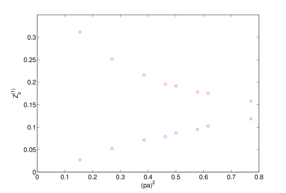
Figure 2: Computation at one loop of $Z_{s}$. The anomalous dimension at one loop is different from zero, and the measure shows a logarithmic divergence (red points). In blue the results after the $\gamma_{s}\log{\hat{p}}^{2}$ contribution subtraction.

In figure 3 we present the preliminar result for the critical mass at three loop, $m_{cr}^{(3)}$. This quantity doesn’t present either vector structure or $\log$ divergences. Critical mass is a byproduct of all the previous computations. The introduction of this counterterm is needed in the computation of the next loop quantities.

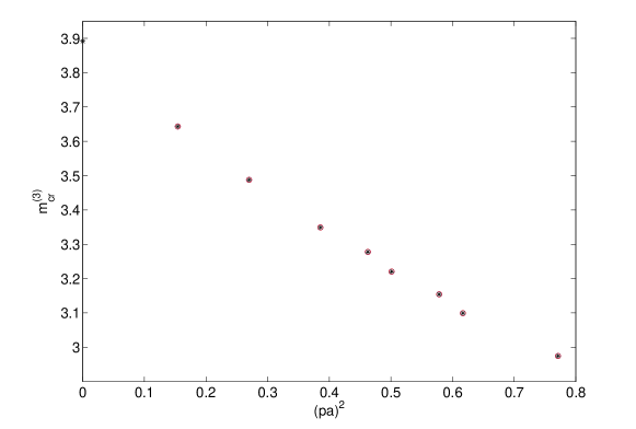
Figure 3: Preliminar result for the critical mass at three loop. In red the result of measurements, in black the result of the fitting procedure.

6 Work in progress

The aim of this work is to compute high order renormalization coefficients for masses, fields and bilinears for different actions. Analytic results are known at most up to 2 loops, while there are NSPT results for Wilson gauge-Wilson fermions up to 3 loops at various $n_{f}$. We are in the process of taking into account $pL$ effects for the latter action. We are now applying the method also to Tree Level Symanzik (current work) and Iwasaki gauge actions. For these actions we’re also interested in computing the $n_{f}$ dependence. Current data are obtained from $32^{4}$ lattices measured on an APE machine, while a C++ code is working on smaller lattices on standard workstations.

References

- [1] G. Martinelli, C. Pittori, C. T. Sachrajda, M. Testa and A. Vladikas, Nucl. Phys. B 445 (1995) 81 [arXiv:hep-lat/9411010].
- [2] M. Luscher, R. Narayanan, P. Weisz and U. Wolff, Nucl. Phys. B 384, 168 (1992) [arXiv:hep-lat/9207009].
- [3] B. Blossier et al. [European Twisted Mass Collaboration], JHEP 0804 (2008) 020 [arXiv:0709.4574 [hep-lat]].
- [4] F. Di Renzo and L. Scorzato, JHEP 0410 (2004) 073 [arXiv:hep-lat/0410010].
- [5] G. Parisi and Y. s. Wu, Sci. Sin. 24, 483 (1981).
- [6] F. Di Renzo, V. Miccio, L. Scorzato and C. Torrero, Eur. Phys. J. C 51 (2007) 645 [arXiv:hep-lat/0611013].
- [7] J. A. Gracey, Nucl. Phys. B 662 (2003) 247 [arXiv:hep-ph/0304113].
- [8] C. T. H. Davies et al., Phys. Rev. D 37 (1988) 1581.
- [9] H. Kawai, R. Nakayama and K. Seo, Nucl. Phys. B 189 (1981) 40.
- [10] S. Aoki, K. i. Nagai, Y. Taniguchi and A. Ukawa, Phys. Rev. D 58 (1998) 074505 [arXiv:hep-lat/9802034].