Towards a precise determination of the topological
susceptibility in the SU(3) Yang-Mills theory

Abstract

An ongoing effort to compute the topological susceptibility for the $SU(3)$ Yang-Mills theory in the continuum limit with a precison of about $2\%$ is reported. The susceptibility is computed by using the definition of the charge suggested by Neuberger fermions for two values of the negative mass parameter s. Finite volume and discretization effects are estimated to meet this level of precision. The large statistics required has been obtained by using PCs of the INFN-GRID.Simulations with larger lattice volumes are necessary in order to better understanding the continuum limit at small lattice spacing values.

1 Introduction

We continue our numerical study on the lattice of the topological charge distribution in the $SU(3)$ Yang-Mills theory adopting the definition suggested by Neuberger fermions as discussed in a series of papers [1]-[6].
Recent numerical studies on this subject can be found in refs.[7, 8, 9] and ref. [10]. In the last paper a systematic study at different volumes and values of the lattice spacing was performed in order to obtain a reliable determination of the topological susceptibility, the first cumulant of the distribution, at the $5\%$ level in the continuum limit at infinite volume. The result supports the Witten-Veneziano explanation for the large mass of the ${\eta}^{\prime}$.
The aim of refs [11, 12] was to look for non-gaussianities in the topological charge distribution of the $SU(3)$ Yang-Mills theory. This is particularly challenging since the contribution of the $n^{\mathrm{th}}$ cumulant to the charge distribution is suppressed as $V^{n-1}$ in its asymptotic expansion, even though the cumulant itself is a quantity of $O(1)$ in the infinite volume limit. It is also worth noting that in order to search for such very small sub-leading effects it is necessary to be sure that all the systematics of the calculation cannot either simulate or hide the effect, and therefore a solid theoretical framework, such as the one provided by the topological charge definition suggested from Ginsparg-Wilson fermions, is indispensable. In ref. [10] three different lattices at the same physical volume of $\sim(1.12{\rm fm})^{4}$ but with about ten time more statistics than in ref. [10], i.e. roughly $3\cdot 10^{4}$ configurations, were studied in order to be able to unveil deviations from the Gaussian distribution. Significant deviations were found, the second cumulant of the distribution gets a value definitively different from zero within errors, and the distribution function agrees at that precision level with a first order modification in $V^{-1}$ of the Gaussian (Edgeworth expansion). The results clearly disfavour the $\theta$ behaviour of the vacuum energy predicted by dilute instanton models, while they are compatible with the expectation from the large $N_{c}$ expansion.

Here we present preliminary results for a measurement on the lattice of the topological susceptibility at the $2\%$ level. In order to keep finite volume and discretization effects below this level of precision, we have exploited data produced in ref. [12] together with new data generated by additional lattices as described below.

All the above challenging Monte Carlo calculation have been made possible by important improvements in algorithms which guarantee the reliability and the feasibility of high statistics. In particular we have used algorithms for zero mode counting with no contamination from quasi zero modes, optimized to run fast on a single processor [13]. The considerable amount of computer time needed has been granted to us by the INFN GRID project. It allowed us to use the computer resources shared in the scientific Italian network provided by INFN along these years. We have also taken in advantage of the computer resources of the Italian organization COMETA.

2 Theoretical framework

In this section we summarize our notation and the necessary theoretical framework, for a complete discussion see for example [12]. In the following we use the plaquette Wilson action of the $SU(3)$ gauge field. The massless lattice Neuberger-Dirac operator $D$ satisfies the Ginsparg-Wilson relation [1, 2]

$$\gamma_{5}D+D\gamma_{5}=\bar{a}D\gamma_{5}D\;,$$ (1)

and the associated topological charge density can be defined as

$$a^{4}q(x)=-\frac{\bar{a}}{2}\,\mathrm{Tr}\Big{[}\gamma_{5}D(x,x)\Big{]},$$ (2)

where ${\bar{a}}=a/(1+s)$, $a$ is the lattice spacing and $s$ is the negative mass parameter. The latter has been fixed in our calculation at the values $s=0.4$ for the study of the volume effects and to $s=0.0$ and $s=0.4$ for the study of the discretization behaviour. The topological charge is obtained from the lattice by computing on each gauge configuration the number and the chirality of the zero modes of $D$ with the algorithm proposed in Ref. [13]. The index $\nu$ of the Dirac operator

$$\nu=n_{+}-n_{-}$$ (3)

is directly related to the topological charge $Q$

$$\nu=Q=a^{4}\sum_{x}q(x)\;.$$

In the Euclidean space-time the ground-state energy $F(\theta)$ is defined as

$$e^{-F(\theta)}=\langle e^{i\theta Q}\rangle\;,$$ (4)

where, as usual, $\langle\dots\rangle$ indicates the path-integral average (our normalization is $F(0)=0$). In the large volume regime $F(\theta)$ is proportional to the size $V$ of the system, a direct consequence of the fact that the topological charge operator $Q$ is the four-dimensional integral of a local density. The function $F(\theta)$ is related to the probability of finding a gauge field configuration with topological charge $Q=\nu$ by the Fourier transform

$$P_{\nu}=\int_{-\pi}^{\pi}\frac{d\theta}{2\pi}e^{-i\theta\nu}e^{-F(\theta)}\;.$$ (5)

Large $N_{c}$ arguments with $N_{c}$ being the number of colors, suggest that the fluctuations of the topological charge are of quantum non-perturbative nature. The $\theta$ dependence of the vacuum energy is expected at leading order in $1/N_{c}$, and the normalized cumulants

$${C}_{n}=(-1)^{n+1}\frac{1}{V}\frac{d^{2n}}{d\theta^{2n}}F(\theta)\Big{|}_{\theta=0}\qquad n=1,2,\dots\;,$$ (6)

which should scale asymptotically as $N_{c}^{2-2n}$, have to be determined with a non-perturbative computation. The normalized cumulants ${C}_{n}$ can thus be defined as the integrated connected correlation functions of $n$ charge densities (correlation functions of an odd number of topological charges vanish thanks to the invariance of the theory under parity):

$${C}_{n}=\frac{a^{8n}}{V}\sum_{x_{1},\dots,x_{2n}}\langle q(x_{1})\dots q(x_{2n})\rangle^{\mathrm{con}}\;.$$ (7)

They have an unambiguous finite continuum limit which is independent of the details of the regularization [14, 5, 6]. At finite lattice spacing they are affected by discretization errors which start at $O(a^{2})$.

The Monte Carlo technique adopted here generates the gauge configurations with a probability density proportional to $e^{-S_{\mathrm{YM}}}$, with $S_{\mathrm{YM}}$ being the chosen discretization of the Yang–Mills action. This algorithm performs an importance sampling of the topological charge with the probability distribution given in Eq. (5). A statistical signal for the $n^{\mathrm{th}}$ cumulant is then obtained when the number of configurations in the sample is high enough to be sensitive to terms suppressed as $V^{n-1}$ in the asymptotic expansion. For instance, the estimators of the first two cumulants

$$\overline{Q^{2}} = \frac{1}{N}\sum_{i=1}^{N}\nu^{2}_{i}\;,$$ (8)

$$\overline{Q^{4,}}\,\!^{\mathrm{con}} = \frac{1}{N}\sum_{i=1}^{N}\nu^{4}_{i}-3\left(\frac{1}{N}\sum_{i=1}^{N}\nu^{2}_{i}\right)^{2}\;,$$ (9)

with $\nu_{i}$ being the value of the topological charge for a given gauge configuration and $N$ the total number of configurations, have variances which, up to sub-leading corrections, are given by $(2\sigma^{4}+\sigma^{2}\tau)/N$ and $(24\sigma^{8}+72\sigma^{6}\tau)/N$ respectively being $\sigma^{2}=V{C}_{1}$ and $\tau={C}_{2}/{C}_{1}$.

3 Lattice data and results

Lat	$\beta$	$L/a$	$r_{0}/a$	$L$[fm]	$N$	$\langle Q^{2}\rangle$	$r_{0}^{4}\chi$
${\rm A}_{1}$	$6.0$	$12$	$5.368$	$1.12$	$34800$	$1.627(13)$	$0.0652(12)$
${\rm B}_{0}$	$5.9138$	$12$	$4.601$	$1.30$	$10000$	$3.271(47)$	$0.0707(15)$
${\rm B}_{1}$	$6.0$	$14$	$5.368$	$1.30$	$30000$	$3.097(26)$	$0.0669(12)$
${\rm B}_{2}$	$6.0808$	$16$	$6.135$	$1.30$	$10000$	$2.914(43)$	$0.0630(14)$
${\rm B}_{3}$	$6.1568$	$18$	$6.902$	$1.30$	$10000$	$2.843(42)$	$0.0615(14)$
${\rm C}_{1}$	$6.0$	$16$	$5.368$	$1.49$	$10000$	$5.314(75)$	$0.0673(14)$
${\rm D}_{1}$	$6.0$	$18$	$5.368$	$1.60$	$10000$	$8.40(12)$	$0.0664(14)$
${\cal B}_{0}$	$5.9138$	$12$	$4.601$	$1.30$	$10000$	$2.501(36)$	$0.0541(11)$
${\cal B}_{1}$	$6.0$	$14$	$5.368$	$1.30$	$10000$	$2.761(40)$	$0.0597(13)$
${\cal B}_{2}$	$6.0808$	$16$	$6.135$	$1.30$	$10000$	$2.723(40)$	$0.0589(13)$
${\cal B}_{3}$	$6.1568$	$18$	$6.902$	$1.30$	$10000$	$2.788(40)$	$0.0602(14)$

Table 1: Simulation parameters and results.The first seven lattices are generated with the parameter value $s=0.4$, while the other four, under the horizontal line, are for $s=0.0$. The topological susceptibility is given by $\chi={\langle Q^{2}\rangle/V}=C_{1}$.

The properties of the lattices considered and the results obtained for the topological susceptibility are reported in Table 1.

On the sets ${\rm A}_{1},\,{\rm B}_{0},\,{\rm B}_{1},\,{\rm B}_{2},\,{\rm B}_{3},\,{\rm C}_{1}$ and ${\rm D}_{1}$ the topological charge is computed with $s=0.4$, while it is determined with $s=0.0$ on the lattices ${\cal B}_{0},\,{\cal B}_{1},\,{\cal B}_{2}$ and ${\cal B}_{3}$.

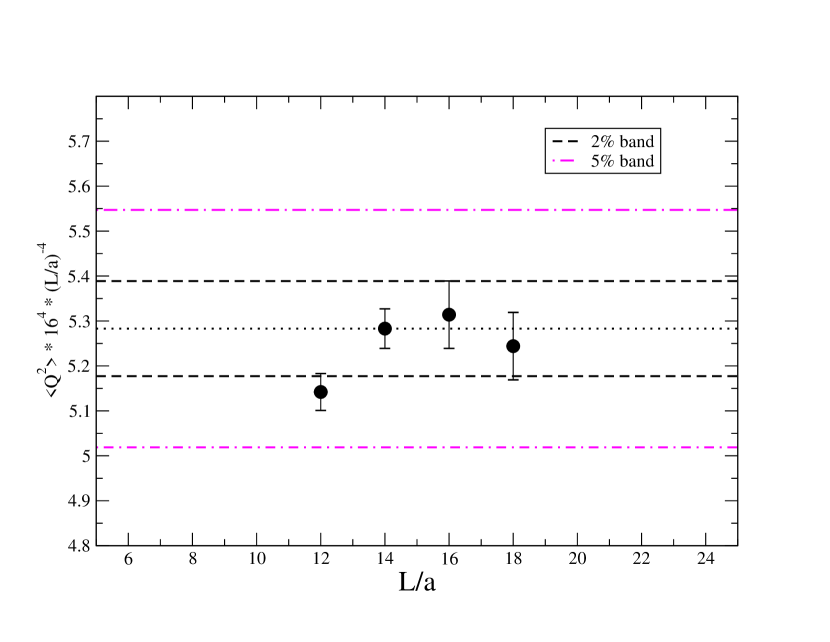
Figure 1: Rescaled topological charge as a function of the lattice size. Bands of $\pm 2\%$ and $\pm 5\%$ centered at the value measured at $L=14$ are also shown.

In order to estimate the magnitude of finite size effects we have considered four lattices (${\rm A}_{1}$, ${\rm B}_{1}$, ${\rm C}_{1}$, ${\rm D}_{1})$) at the same value of the coupling constant corresponding to $\beta=6.0$ and at the same value of the negative mass parameter $s=0.4$. The values of the topological charge rescaled with respect to the reference volume of $16^{4}$ are shown in Fig. 1. It is rather clear that for these volumes the results are scattered in a $2\%$ band centered around the point with $L/a=14$. While we cannot exclude that the point at $L/a=12$ turns out to be lower with respect to the others due to a statistical fluctuation only, the other three points indicate clearly that finite size effects are within our statistical errors for volumes larger or equal than $(1.3\;{\rm fm})^{4}$.
Building on this result, the coupling constant of the other seven lattices have been chosen so that the lattice linear extent is fixed to be $1.3$ fm, while the values of the coupling constant and of the negative mass $s$ are chosen in order to properly estimate discretization errors at this level of precision. The results for the topological susceptibility for all lattices with linear extent of $1.3$ fm are shown in Fig. 2 as a function of $(a/r_{0})^{2}$. The data show a clear trend to converge to the same value in the continuum limit within the statistical precision reached. Nevertheless a better understanding of the behaviour at small lattice spacing values, i.e. larger lattice volumes, seems to be necessary in order to improve the continuum limit study. In fact, data at the $2\%$ level of error indicate a statistically non-negligible (and non-universal) contributions of terms of $O(a^{4})$ to the behaviour of the two curves in this range of values of $\beta$. Simulations at larger values of $\beta$ are underway.

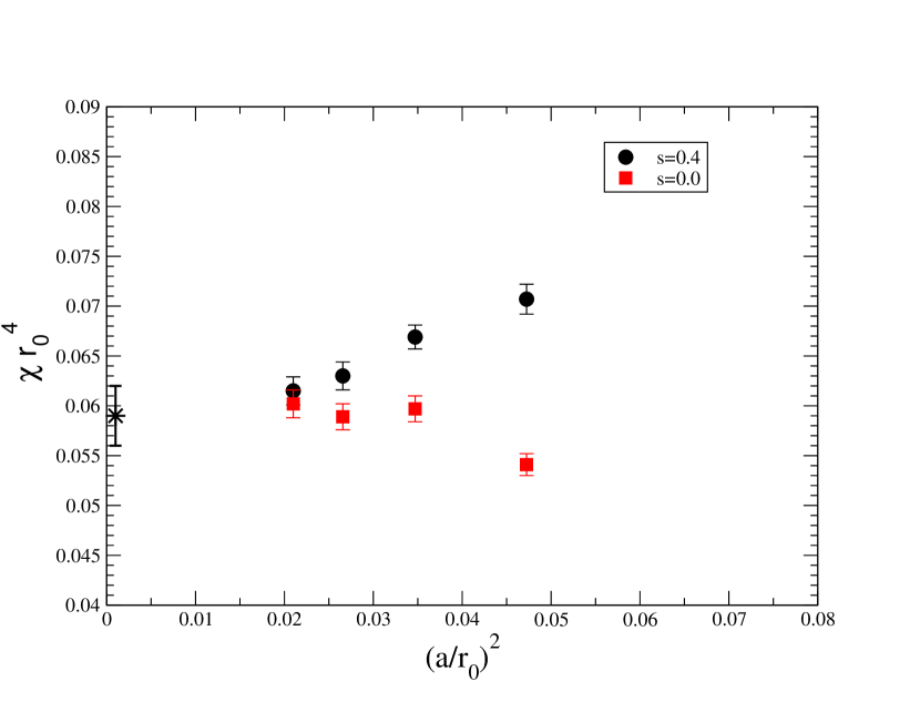
Figure 2: Topological susceptibility as a function of the square of the lattice spacing at a fixed value of the lattice size $L=1.304$ fm: data at mass parameter $s=0$ (squares) and $s=0.4$ (circles) are shown. The continuum limit point is the result quoted in ref. [10].

4 Acknowledgments

We warmly thank G. Andronico for the great organization of Theophys, the virtual organization of INFN Grid Project for theoretical physics. We thank A. De Salvo and A. Colla of the INFN sez. Rome for the continuous effort in helping us during the accomplishment of the project and the COMETA organization for having opened their virtual organization to us.

References

- [1] H. Neuberger, Phys. Lett. B417, 141, (1998), hep-lat/9707022.
- [2] H. Neuberger, Phys. Rev. D57, 5417, (1998), hep-lat/9710089.
- [3] P. Hasenfratz, V. Laliena, F. Niedermayer, Phys. Lett. B427, 125, (1998), hep-lat/9801021.
- [4] M. Lüscher, Phys. Lett. B428, 342, (1998), hep-lat/9802011.
- [5] L. Giusti, G. C. Rossi, M. Testa, Phys. Lett. B587, 157, (2004), hep-lat/0402027.
- [6] M. Lüscher, Phys. Lett. B593, 296, (2004), hep-th/0404034.
- [7] R. G. Edwards, U. M. Heller and R. Narayanan, Phys. Rev. D 59 (1999) 094510, hep-lat/9811030.
- [8] L. Giusti, M. Lüscher, P. Weisz, H. Wittig, JHEP 11, 023 (2003), hep-lat/0309189.
- [9] L. Del Debbio, C. Pica, JHEP 0402, 003 (2004), hep-lat/0309145.
- [10] L. Del Debbio, L. Giusti, C. Pica, Phys. Rev. Lett. 94:032003 (2005), hep-th/0407052.
- [11] L. Giusti, S. Petrarca, B. Taglienti, PoS LAT2006:058,2006,hep-lat/0705.3151.
- [12] L. Giusti, S. Petrarca, B. Taglienti, Phys.Rev. D.76:094510,2007,hep-th/0705.2352.
- [13] L. Giusti, C. Hoelbling, M. Luscher, H. Wittig, Comput. Phys. Commun. 153, 31 (2003), hep-lat/0212012.
- [14] L. Giusti, G. C. Rossi, M. Testa, G. Veneziano, Nucl. Phys. B628, 234, (2002), hep-lat/0108009.