Spin-resolved scattering through spin-orbit nanostructures in graphene

Abstract

We address the problem of spin-resolved scattering through spin-orbit nanostructures in graphene, i.e., regions of inhomogeneous spin-orbit coupling on the nanometer scale. We discuss the phenomenon of spin-double refraction and its consequences on the spin polarization. Specifically, we study the transmission properties of a single and a double interface between a normal region and a region with finite spin-orbit coupling, and analyze the polarization properties of these systems. Moreover, for the case of a single interface, we determine the spectrum of edge states localized at the boundary between the two regions and study their properties.

I introduction

Graphenegeim ; kim — a single layer of carbon atoms arranged in a honeycomb lattice — has attracted huge attention in the physics community because of many unusual electronic, thermal and nanomechanical properties.reviews ; beenakker:2008 In graphene the Fermi surface, at the charge neutrality point, reduces to two isolated points, the two inequivalent corners $K$ and $K^{\prime}$ of the hexagonal Brillouin zone of the honeycomb lattice. In their vicinity the charge carriers form a gas of chiral massless quasiparticles with a characteristic conical spectrum. The low-energy dynamics is governed by the Dirac-Weyl (DW) equationsemenoff ; divincenzomele in which the role of speed of light is played by the electron Fermi velocity. The chiral nature of the quasiparticles and their linear spectrum lead to remarkable consequences for a variety of electronic properties as weak localization, shot noise, Andreev reflection, and many others. Also the behavior in a perpendicular magnetic field discloses new physics. Graphene exhibits a zero-energy Landau level, whose existence gives rise to an unconventional half-integer quantum Hall effect, one of the peculiar hallmarks of the DW physics.

Driven by the prospects of using this material in spintronic applications,spintronics ; Trauzettel:2008 the study of spin transport is one of the most active field in graphene research.expspin1 ; expspin2 ; expspin3 ; expspin4 ; expspin5 ; expspin6 Several experiments have recently demonstrated spin injection, spin-valve effect, and spin-coherent transport in graphene, with spin relaxation length of the order of few micrometers.expspin2 ; expspin6 In this context a crucial role is played by the spin-orbit interaction. In graphene symmetries allow for two kinds of spin-orbit coupling (SOC).kane:2005 The intrinsic SOC originates from carbon intra-atomic SOC. It opens a gap in the energy spectrum and converts graphene into a topological insulator with a quantized spin-Hall effect.kane:2005 This term has been estimated to be rather weak in clean flat graphene.soguinea ; so2 ; so3 ; so4 The extrinsic Rashba-like SOC originates instead from interactions with the substrate, presence of a perpendicular external electric field, or curvature of graphene membrane.soguinea ; so2 ; so3 ; so5 This term is believed to be responsible for spin polarizationrashbagraphene and spin relaxationguinea2009 ; ertler:2009 physics in graphene. Optical-conductivity measurements could provide a way to determine the respective strength of both SOCs.philip

In this article we address the problem of ballistic spin-dependent scattering in the presence of inhomogeneous spin-orbit couplings. Our main motivation stems from a recent experiment that reported a large enhancement of Rashba SOC splitting in single-layer graphene grown on Ni(111) intercalated with a Au monolayer.varykhalov:2008 Further experimental results show that the intercalation of Au atoms between graphene and the Ni substrate is essential in order to observe sizable Rashba effect.rader:2009 ; varykhalov:2009 The preparation technique of Ref. varykhalov:2008, seems to provide a system with properties very close to those of freestanding graphene in spite of the fact that graphene is grown on a solid substrate. The presence of the substrate does not seem to fundamentally alter the electronic properties observed in suspended systems, i.e., the existence of Dirac points at the Fermi energy and the gapless conical dispersion in their vicinity.

These results suggest that a certain degree of control on the SOC can be achieved by appropriate substrate engineering, with variations of the SOC strength on sub-micrometer scales, without spoiling the relativistic gapless nature of quasiparticles. This could pave the way for the realization of spin-optics devices for spin filtration and spin control for DW fermions in graphene. An optimal design would require a detailed understanding of the spin-resolved ballistic scattering through such spin-orbit nanostructures, which is the aim of this paper.

The problem of spin transport through nanostructures with inhomogeneous SOC has already been thoroughly studied in the case of two-dimensional electron gas in semiconductor heterostructures with Rashba SOC.marigliano1 ; khodas ; marigliano2 Here the Rashba SOC rashba:1960 — arising from the inversion asymmetry of the confinement potential — couples the electron momentum to the spin degree of freedom and thereby lifts the spin degeneracy. In this case, a region with finite SOC between two normal regions has properties similar to biaxial crystals: an electron wave incident from the normal region splits at the interface and the two resulting waves propagate in the SO region with different Fermi velocities and momenta. marigliano1 This effect — analogous to the optical double-refraction — produces an interference pattern when the electron waves emerge in the second normal region. Moreover, electrons that are injected in an spin unpolarized state emerge from the SO region in a partially polarized state.

Here we shall focus on the two simplest examples of SO nanostructures in graphene: (i) a single interface between two regions with different strengths of SOC; (ii) a SOC barrier, or double interface, i.e., a region of finite SOC in between two regions with vanishing SOC.

Our analysis shows — in analogy to the case of 2DEG — that the ballistic propagation of carriers is governed by the spin-double refraction. We find that the scattering properties of the structure strongly depend on the injection angle. As a consequence, an initially unpolarized DW quasiparticle emerges from the SOC barrier with a finite spin polarization. In analogy to the edge states in the quantum spin-Hall effect,kane:2005 we also consider the possibility of edge states localized at the interface between regions with and without SOC.

This paper is organized as follows. In Sec. II we introduce the model and the transfer matrix formalism used in the rest of the paper. In Sec. III we discuss the scattering problem at a single interface and the spectrum of edge states. In Sec. IV we address the case of a double interface — a SOC barrier — and the final Sec. V is devoted to the discussion of results and conclusions.

II Model and Formalism

Figure 1: (Color online) Illustration of the kinematics of the scattering at a N-SO interface in graphene. The circles represent constant energy contours.

We consider a clean graphene sheet in the $xy$-plane with SOCskane:2005 ; soguinea ; rashbagraphene ; stauber:2009 ; yamakage:2009 inhomogeneous along the $x$-direction. We shall restrict ourselves to a single-particle picture and neglect electron-electron interaction effects. The length scale over which the SOCs vary is assumed to be much larger than graphene’s lattice constant ($a=0.246$ nm) but much smaller than the typical Fermi wavelength of quasiparticles $\lambda_{\text{F}}$. Since close to the Dirac points $\lambda_{\text{F}}\sim 1/|E|$, at low energy $E$ this approximation is justified. This assumption ensures that we can use the continuum DW description, in which the two valleys are not coupled. Yet close to a Dirac point we can approximate the variation of SOCs as a sharp change. Focusing on a single valley, the single-particle Hamiltonian reads

$$\mathcal{H} =v_{\text{F}}\ {\bm{\sigma}}\cdot{\bf p}+\mathcal{H}_{\text{SO}},$$ (1)

$$\mathcal{H}_{\text{SO}} =\frac{\lambda(x)}{2}\left({\bm{\sigma}}\times{\bf s}\right)_{z}+\Delta(x)\sigma_{z}s_{z},$$ (2)

where $v_{\text{F}}\approx 10^{6}$ m/s is the Fermi velocity in graphene. In the following we set $\hbar=v_{\text{F}}=1$. The vector of Pauli matrices $\bm{\sigma}=(\sigma_{x},\sigma_{y})$ [resp. ${\bf s}=(s_{x},s_{y})$] acts in sublattice space [resp. spin space]. The term $\mathcal{H}_{\text{SO}}$ contains the extrinsic or Rashba SOC of strength $\lambda$ and the intrinsic SOC of strength $\Delta$. While experimentally the Rashba SOC can be enhanced by appropriate optimization of the substrate up to values of the order of $14$ meV, varykhalov:2008 the intrinsic SOC seems at least two orders of magnitude smaller. Yet, the limit of large intrinsic SOC is of considerable interest since in this regime graphene becomes a topological insulator.kane:2005 Thus in this paper we shall not restrict ourself to the experimentally relevant regime $\lambda\gg\Delta$ but consider also the complementary regime.

The wave function $\Psi$ is expressed as

$$\Psi^{\text{T}}=(\Psi_{A\uparrow},\Psi_{B\uparrow},\Psi_{A\downarrow},\Psi_{B\downarrow}),$$

where the superscript ${}^{\text{T}}$ denotes transposition. Spectrum and eigenspinors of the Hamiltonian (1) with uniform SOCs are briefly reviewed in Appendix A. The spectrum consists of four branches $E_{\alpha,\epsilon}({\bf k})$ labelled by the two quantum numbers $\epsilon=\pm 1$ and $\alpha=\pm 1$. Here, the first distinguishes particle and hole branches, the second gives the sign of the expectation value of the spin projection along the in-plane direction perpendicular to the propagation direction ${\bf k}$. The spectrum strongly depends on the ratio

$$\eta=\frac{\Delta}{\lambda}.$$ (3)

For $\eta>1/2$ a gap separates particle and hole branches. The gap closes at $\eta=1/2$ and for $\eta<1/2$ one particle branch and one hole branch are degenerate at ${\bf k}=0$ (see Fig. 8 in App. A).

We now briefly summarize the transfer matrix approach employed in this paper to solve the DW scattering problem. mckellar:1987 ; peeters ; luca1 ; luca2 We assume translational invariance in the $y$-direction, thus the scattering problem for the Hamiltonian (1) reduces to an effectively one-dimensional (1D) one. The wave function factorizes as $\Psi(x,y)=\text{e}^{\text{i}k_{y}y}\chi(x)$, where $k_{y}$ is the conserved $y$-component of the momentum, which parameterizes the eigenfunctions of the Hamiltonian of given energy $E$.

For simplicity we consider piecewise constant profiles of SOCs, and solve the DW equation in each region of constant couplings. Then we introduce the $x$-dependent $4\times 4$ matrix $\Omega(x)$, whose columns are given by the components of the independent, normalized eigenspinor of the 1D DW Hamiltonian at fixed energy.footnote1 Due to the continuity of the wave function at each interface between regions of different SOC, the wave function on the left of the interface can be expressed in terms of the wave function on the right via the transfer matrix

$$\mathcal{M}=\left[\Omega(x_{0}^{-})\right]^{-1}\Omega(x_{0}^{+}),$$ (4)

where $x_{0}$ is the position of the interface and $x_{0}^{\pm}=x_{0}\pm\delta$ with infinitesimal positive $\delta$. The condition $\det\mathcal{M}=1$ guarantees conservation of the probability current across the interface. The generalization to the case of a sequence of $N$ interfaces at positions $x_{i}$, $i=1,\dots,N$, is straightforward since the transfer matrices relative to individual interfaces combine via matrix multiplication:

$$\mathcal{M}=\prod_{i=1}^{N}\left[\Omega(x_{i}^{-})\right]^{-1}\Omega(x_{i}^{+}).$$ (5)

From the transfer matrix it is straightforward to determine transmission and reflection matrices, which encode all the relevant information on the scattering properties.

III The N-SO interface

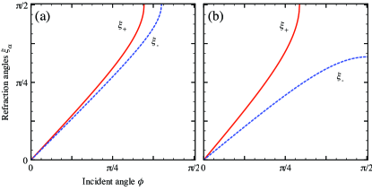
Figure 2: (Color online) Refraction angles as function of the incidence angle for fixed energy and fixed SOCs. Panel (a): $E=5$, $\lambda=0.5$, $\Delta=2$; panel (b): $E=5$, $\lambda=2$, $\Delta=0.5$.

First we concentrate on the elastic scattering problem at the interface separating a normal region N ($x<0$), where SOCs vanish, and a SO region ($x>0$), where SOCs are finite and uniform.

We consider a quasiparticle of energy $E$, with $E$ assumed positive for definiteness and outside the gap possibly opened by SOCs. This quasiparticle incident from the normal region is characterized by the $y$-component of the momentum, or equivalently, the incidence angle $\phi$ measured with respect to the normal at the interface, see Fig. 1. Conservation of $k_{y}$ implies that

$$k_{y}^{\text{N}} =E\sin\phi=E_{\alpha}\sin\xi_{\alpha}=k_{y}^{\text{SO}}$$ (6a)

$$k_{x}^{\text{N}} =E\cos\phi$$ (6b)

$$k_{x\alpha}^{\text{SO}} =E_{\alpha}\cos\xi_{\alpha}$$ (6c)

where $\alpha=\pm 1$ and $E_{\alpha}=\sqrt{(E-\Delta)(E+\Delta-\alpha\lambda)}$. The refraction angles $\xi_{\alpha}$ are fixed by momentum conservation along the interface (6a) and read

$$\xi_{\alpha}=\arcsin\left(\frac{E}{E_{\alpha}}\sin\phi\right)\,.$$ (7)

Figure 1 illustrates the refraction process at the N-SO interface. The incident wave function, assumed to have fixed spin projection in the $z$-direction, in the SO region splits in a superposition of eigenstates of the SOCs Hamiltonian corresponding to states in the different branches of the spectrum. These eigenstates propagate along two distinct directions characterized by the angles $\xi_{\alpha}$, whose difference depends on SOC and is an increasing function of the incidence angle, see Fig. 2. The angles $\xi_{\alpha}$ coincide only for normal incidence or for $\lambda=0$.

Equation (7) implies that there exists a critical angle for each of the two modes given by

$$\tilde{\phi}_{\alpha}=\arcsin\left(\frac{E_{\alpha}}{E}\right).$$ (8)

For $\phi$ larger than both critical angles $\tilde{\phi}_{\alpha}$, the quasiparticle is fully reflected, since there are no available transmission channels in the SO region. For $\phi$ in between the two critical angles the quasiparticle transmits only in one channel.footnote2

After this qualitative discussion of the kinematics, we now present the exact solution of the scattering problem. In the N region $x<0$ a normalized scattering state of energy $E>0$, incident from the left on the interface with incidence angle $\phi$ and spin projection $s$ is given by

$$\chi_{\text{N}}(x)= \left[\delta_{\uparrow,s}|\!\uparrow\rangle+\delta_{\downarrow,s}|\!\downarrow\rangle\right]\begin{pmatrix}1\\ \text{e}^{\text{i}\phi}\end{pmatrix}\frac{\text{e}^{\text{i}k_{x}x}}{\sqrt{2v_{\text{F}}^{x}}}$$

$$+\left[r_{\uparrow s}|\!\uparrow\rangle+r_{\downarrow s}|\!\downarrow\rangle\right]\begin{pmatrix}1\\ -\text{e}^{-\text{i}\phi}\end{pmatrix}\frac{\text{e}^{-\text{i}k_{x}x}}{\sqrt{2v_{\text{F}}^{x}}},$$ (9)

where $k_{x}\equiv k_{x}^{\text{N}}$ (cf. Eq. 6b). Here the index $s=\uparrow,\downarrow$ specifies the spin projection of the incoming quasiparticle with $|\!\!\uparrow\rangle$ and $|\!\!\downarrow\rangle$ eigenstates of $s_{z}$ and $\delta_{i,j}$ is the Kronecker delta. The velocity $v_{\text{F}}^{x}=\cos\phi$ is included to ensure proper normalization of the scattering state. The complex coefficients $r_{s^{\prime}s}$ are reflection probability amplitudes for a quasiparticle with spin $s$ to be reflected with spin $s^{\prime}$. The associated matrix $\Omega_{\text{N}}(x)$ reads

$$\Omega_{\text{N}}(x) =\frac{1}{\sqrt{2v_{\text{F}}^{x}}}$$

$$\begin{pmatrix}\text{e}^{\text{i}k_{x}x}&\text{e}^{-\text{i}k_{x}x}&0&0\\ \text{e}^{\text{i}(k_{x}x+\phi)}&-\text{e}^{-\text{i}(k_{x}x+\phi)}&0&0\\ 0&0&\text{e}^{\text{i}k_{x}x}&\text{e}^{-\text{i}k_{x}x}\\ 0&0&\text{e}^{\text{i}(k_{x}x+\phi)}&-\text{e}^{-\text{i}(k_{x}x+\phi)}\end{pmatrix}.$$

Similarly the wave function in the SO region ($x>0$) can be expressed in general form as

$$\chi_{\text{SO}}(x) =\frac{1}{\sqrt{v_{++}^{x}}}\left[t_{+}\psi_{++}(x)+r_{+}\bar{\psi}_{++}(x)\right]$$

$$+\frac{1}{\sqrt{v_{-+}^{x}}}\left[t_{-}\psi_{-+}(x)+r_{-}\bar{\psi}_{-+}(x)\right]$$ (10)

where $t_{\pm}$ (resp. $r_{\pm}$) are complex amplitudes for right-moving (resp. left-moving) states. The coefficient $t_{\alpha}$ represents the transmission amplitude into mode $\alpha$. The wave functions $\psi_{\alpha+}$ and the Fermi velocities $v_{\alpha+}^{x}$ in the SO region are obtained from the expressions given in App. A with the replacement $k_{x}\to k_{x\alpha}^{\text{SO}}$, where for notational simplicity the label SO will be understood. The wave functions $\bar{\psi}_{\alpha+}$ are in turn obtained from $\psi_{\alpha+}$ by replacing $k_{x\alpha}\to-k_{x\alpha}$. The matrix $\Omega_{\text{SO}}(x)$ then reads

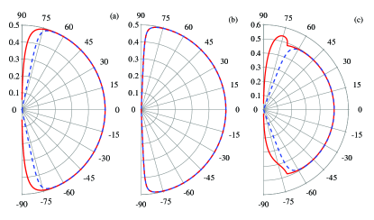
Figure 3: (Color online) Angular dependence of the transmission probabilities $T_{+\uparrow}$ (blue dashed line) and $T_{-\uparrow}$ (red solid line) at energy $E=2.5$. The SOC are fixed as follows: (a) $\lambda=0.1$ and $\Delta=0$, (b) $\lambda=0$ and $\Delta=0.1$, and (c) $\lambda=0.5$ and $\Delta=0.1$.

$$\Omega_{\text{SO}}(x) =$$ (11)

$$\begin{pmatrix}\text{e}^{-\text{i}\xi_{+}-\frac{\theta_{+}}{2}}&-\text{e}^{\text{i}\xi_{+}-\frac{\theta_{+}}{2}}&\text{e}^{-\text{i}\xi_{-}-\frac{\theta_{-}}{2}}&-\text{e}^{\text{i}\xi_{-}-\frac{\theta_{-}}{2}}\\ \text{e}^{\frac{\theta_{+}}{2}}&\text{e}^{\frac{\theta_{+}}{2}}&\text{e}^{\frac{\theta_{-}}{2}}&\text{e}^{\frac{\theta_{-}}{2}}\\ \text{i}\text{e}^{\frac{\theta_{+}}{2}}&\text{i}\text{e}^{\frac{\theta_{+}}{2}}&-\text{i}\text{e}^{\frac{\theta_{-}}{2}}&-\text{i}\text{e}^{\frac{\theta_{-}}{2}}\\ \text{i}\text{e}^{\text{i}\xi_{+}-\frac{\theta_{+}}{2}}&-\text{i}\text{e}^{-\text{i}\xi_{+}-\frac{\theta_{+}}{2}}&-\text{i}\text{e}^{\text{i}\xi_{-}-\frac{\theta_{-}}{2}}&\text{i}\text{e}^{-\text{i}\xi_{-}-\frac{\theta_{-}}{2}}\end{pmatrix}$$

$$\begin{pmatrix}\mathcal{N}_{+}\text{e}^{\text{i}k_{x+}+x}&0&0&0\\ 0&\mathcal{N}_{+}\text{e}^{-\text{i}k_{x+}x}&0&0\\ 0&0&\mathcal{N}_{-}\text{e}^{\text{i}k_{x-}x}&0\\ 0&0&0&\mathcal{N}_{-}\text{e}^{-\text{i}k_{x-}x}\end{pmatrix}$$

where in the second matrix the normalization factors are defined as $\mathcal{N}_{\alpha}=1/(2\sqrt{v_{\alpha+}\sinh\theta_{\alpha}})$.

According to Eq. (4) the transfer matrix for the single interface problem is given by the matrix product $\mathcal{M}=[\Omega_{\text{N}}(0^{-})]^{-1}\Omega_{\text{SO}}(0^{+})$. From $\mathcal{M}$ we obtain the transmission and the reflection probabilities for a spin-up or spin-down incident quasiparticle:

$$T_{+s} =\displaystyle\left|\frac{\mathcal{M}_{33}\delta_{s,\uparrow}+\mathcal{M}_{13}\delta_{s,\downarrow}}{\mathcal{M}_{13}\mathcal{M}_{31}-\mathcal{M}_{11}\mathcal{M}_{33}}\right|^{2}\Upsilon_{+}(\phi),$$ (12)

$$T_{-s} =\displaystyle\left|\frac{\mathcal{M}_{31}\delta_{s,\uparrow}+\mathcal{M}_{11}\delta_{s,\downarrow}}{\mathcal{M}_{13}\mathcal{M}_{31}-\mathcal{M}_{11}\mathcal{M}_{33}}\right|^{2}\Upsilon_{-}(\phi),$$ (13)

$$R_{\uparrow s} =\displaystyle\left|\frac{\mathcal{M}_{31}\mathcal{M}_{23}-\mathcal{M}_{33}\mathcal{M}_{21}}{\mathcal{M}_{13}\mathcal{M}_{31}-\mathcal{M}_{11}\mathcal{M}_{33}}\right|^{2}\delta_{s,\uparrow}$$

$$\hskip 28.45274pt+\left|\frac{\mathcal{M}_{13}\mathcal{M}_{21}-\mathcal{M}_{11}\mathcal{M}_{23}}{\mathcal{M}_{13}\mathcal{M}_{31}-\mathcal{M}_{11}\mathcal{M}_{33}}\right|^{2}\delta_{s,\downarrow},$$ (14)

$$R_{\downarrow s} =\displaystyle\left|\frac{\mathcal{M}_{31}\mathcal{M}_{43}-\mathcal{M}_{33}\mathcal{M}_{41}}{\mathcal{M}_{13}\mathcal{M}_{31}-\mathcal{M}_{11}\mathcal{M}_{33}}\right|^{2}\delta_{s,\uparrow}$$

$$\hskip 28.45274pt+\left|\frac{\mathcal{M}_{13}\mathcal{M}_{41}-\mathcal{M}_{11}\mathcal{M}_{43}}{\mathcal{M}_{13}\mathcal{M}_{31}-\mathcal{M}_{11}\mathcal{M}_{33}}\right|^{2}\delta_{s,\downarrow},$$ (15)

where $\Upsilon_{\alpha}(\phi)=\theta(\tilde{\phi}_{\alpha}-\phi)\theta(\tilde{\phi}_{\alpha}+\phi)$ with $\theta(x)$ the Heaviside step function. Here, $T_{\alpha s}$ is the probability for an incident quasiparticle with spin projection $s$ to be transmitted in mode $\alpha$ in the SO region. Of course, probability current conservation enforces $T_{+s}+T_{-s}+R_{\uparrow s}+R_{\downarrow s}=1$.

Figures 3 (a)–(c) show the angular dependence of the transmission probabilities for an incident spin-up quasiparticle into the $(+)$ and $(-)$ modes of the SO region for different values of the SOCs. Panel (a) refers to the case of vanishing intrinsic SOC ($\Delta=0$). Here the $(+)$ and the $(-)$ energy bands are separated by a SOC-induced splitting $\Delta E_{\text{ext}}=\lambda$. Therefore at fixed energy the two propagating modes in the SO region have two different momenta, which gives rise to the two different critical angles (cf. Eq. (8) with $\Delta=0$). Panel (b) refers to the case $\lambda=0$, where the SOC opens a gap $\Delta E_{\text{int}}=2\Delta$ between the particle- and the hole-branches, however the $(+)/(-)$-modes remain degenerate. Therefore at fixed energy these modes have the same momentum and, as a consequence, the same critical angles (cf. Eq. (8) for $\lambda=0$ and $\Delta\neq 0$). When both SOCs are finite — the situation illustrated in panel (c) — the transmission probabilities exhibit more structure. For incidence angles smaller than $\tilde{\phi}_{+}$ no particular differences with the cases of panels (a) and (b) are visible. When the $(+)$ mode is closed, an increase (resp. decrease) of the $(-)$ mode transmission is observed for positive (resp. negative) angles, before the transmission drops to zero for incidence angles approaching $\tilde{\phi}_{-}$. The asymmetry between positive and negative angles is reversed if the spin state of the incident quasiparticle is reversed.

These symmetry properties can be rationalized by considering the operator of mirror symmetry through the $x$-axes.zhai:2005 This consists of the transformation $y\to-y$ and at the same time the inversion of the spin and the pseudo-spin states. It reads

$$\mathcal{S}_{y}=(\sigma_{x}\otimes s_{y})R_{y},$$ (16)

where $R_{y}$ transforms $y\to-y$. The operator $\mathcal{S}_{y}$ commutes with the total Hamiltonian of the system $[\mathcal{S}_{y},\mathcal{H}_{0}+\mathcal{H}_{\text{SO}}]=0$, therefore allows for a common basis of eigenstates. For the scattering states in the SO region (III) we have $\mathcal{S}_{y}\chi_{+}(\xi_{+})=\chi_{+}(\xi_{+})$ and $\mathcal{S}_{y}\chi_{-}(\xi_{-})=-\chi_{-}(\xi_{-})$. Instead, it induces the following transformation on the scattering states (III) in the normal region: $\mathcal{S}_{y}\chi_{s}(\phi)=\text{i}\chi_{-s}(-\phi)$. By comparing the original scattering matrix with the $\mathcal{S}_{y}$-transformed one we find that

$$T_{\alpha,s}(\phi)=T_{\alpha,-s}(-\phi)$$ (17)

with $\alpha=\pm$ and $s=\uparrow,\downarrow$, which is indeed the symmetry observed in the plots. The asymmetry of the transmission coefficients occurs only when both SOCs are finite.

III.1 Edge states at the interface

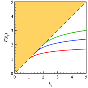
Figure 4: (Color online). Energy dispersion of the edge state at the N-SO interface as a function of the momentum along the interface $k_{y}$ for different values of SOCs. Solution of the transcendental equation is allowed only for $|k_{y}|>|E|$ (white area). In all three cases shown $\eta>1/2$: $\Delta=1$ and $\lambda=0.4$ (lower-red line), $\Delta=1.5$ and $\lambda=0.7$ (middle-blue line), and $\Delta=2$ and $\lambda=0.9$ (upper-green line).

In addition to scattering solutions of the DW equation, it is interesting to study the possibility that edge states exist at the N-SO interface, which propagate along the interface but decay exponentially away from it. The interest in these types of solutions is connected to the study of topological insulators. It has been shown — first by Kane and Melekane:2005 — that a zig-zag graphene nanoribbon with intrinsic SOC supports dissipationless edge states within the SOC gap. In fact, similar states are always expected to exist at the interface between a topologically trivial and a topologically non-trivial insulator. In our case, the latter is represented by graphene with intrinsic SOC. Of course SOC-free graphene is not an insulator, however it is topologically trivial and edge state solutions do arise for $|k_{y}|>|E|$. When $E$ is within the gap in the SO region the corresponding mode is evanescent along the $x$ direction on both sides of the interface. Note that the edge state we find is different from the one discussed in Refs. kane:2005, , stauber:2009, where zig-zag or hard-wall boundary conditions at the edge of the SOC region were imposed.

The wave function on the N side then reads

$$\chi_{\text{N}}(x)=\begin{pmatrix}1\\ \frac{-\text{i}q+\text{i}k_{y}}{E}\end{pmatrix}\left(A|\!\downarrow\rangle+B|\!\uparrow\rangle\right)\text{e}^{qx}$$ (18)

with $q=\sqrt{|k_{y}|^{2}-E^{2}}$. In the SO region the wave function can be written as

$$\chi_{\text{SO}}(x) =C\begin{pmatrix}(-q_{+}+k_{y})\\ \text{i}(E-\Delta)\\ E-\Delta\\ \text{i}(q_{+}+k_{y})\end{pmatrix}\text{e}^{-q_{+}x}+D\begin{pmatrix}(q_{-}-k_{y})\\ -\text{i}(E-\Delta)\\ E-\Delta\\ (q_{-}+\text{i}k_{y})\end{pmatrix}\text{e}^{-q_{-}x}$$

with $q_{\alpha}=\sqrt{k_{y}^{2}-(E-\Delta)(E+\Delta-\alpha\lambda)}$. The continuity of the wave function at the N-SO interface leads to a linear system of equations for the amplitudes $A$ to $D$. The matrix of coefficients must have a vanishing determinant for a non-trivial solution to exist. This condition provides a transcendental equation for the energy of possible edge states, whose solutions are illustrated in Fig. 4  for different values of the intrinsic and extrinsic SOCs. The condition $|k_{y}|>|E|$ implies that solutions only exist outside the shadowed area. In addition, they are allowed only in the case SOCs open a gap in the energy spectrum, which occurs when $\eta>1/2$ (see App. A and Eq. (3)). As can be seen in Fig. 4 the result is quite insensitive to the precise value of the extrinsic SOC.

Edge states exist only for values of the momentum along the interface larger than the intrinsic SOC, i.e., $k_{y}>k_{y}^{\text{min}}=\Delta$. The apparent breaking of time-reversal invariance (the dispersion is not even in $k_{y}$) is due to the fact that we are considering a single-valley theory. The full two-valley SOC Hamiltonian is invariant under time-reversal symmetry, that interchanges the valley quantum number. This invariance implies that solutions for negative values of $k_{y}$ can be obtained by considering the Dirac-Weyl Hamiltonian relative to the other valley. The two counter-propagating edge states live then at opposite valleys and have opposite spin state and realize a peculiar 1D electronic system.

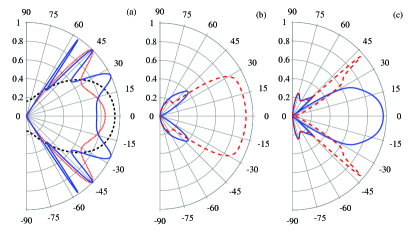
Figure 5: (Color online). Panel (a): Angular plots for $T_{\uparrow\uparrow}$ as a function of the injection angle for $E=2$, $\Delta=1$ and $\lambda=0$. The three lines correspond to different distance between the interfaces: $d=\pi/2$ (dashed black), $d=\pi$ (dotted red), and $d=2\pi$ (solid blue). The spin-precession length is $\ell_{\text{SO}}=\pi$. When $\lambda=0$ the transmission probability in the spin state opposed to the injected spin is always zero. Panel (b) and (c): angular plots of $T_{\uparrow\uparrow}$ (solid-blue) and $T_{\downarrow\uparrow}$ (dashed red) as a function of the injection angle for $E=2$, $\lambda=1$ and $\Delta=0$. The distance between the two interfaces is $d=\pi$ in panel (a) and $d=2\pi$ in panel (b). The spin-precession length is $\ell_{\text{SO}}=2\pi$.

As mentioned in the Introduction, the intrinsic SOC is estimated to be much smaller than the extrinsic one, therefore in a realistic situation one would not expect the opening of a significant energy gap and the presence of edge states. It would be interesting to explore the possibility to artificially enhance the intrinsic SOC, thereby realizing the condition for the occurrence of edge states.

IV The N-SO-N interface

The analysis of the scattering problem on a N-SO interface of the previous section can be straightforwardly generalized to the case of a double N-SO-N interface (SO barrier). Here the transmission matrix $\mathcal{D}$ is given by Eq. (5) with $N=2$. The transmission and the reflection probabilities in the case of a spin-up or -down incident quasiparticle read

$$T_{\uparrow s} =\displaystyle\left|\frac{\mathcal{D}_{33}\delta_{s,\uparrow}+\mathcal{D}_{13}\delta_{s,\downarrow}}{\mathcal{D}_{13}\mathcal{D}_{31}-\mathcal{D}_{11}\mathcal{D}_{33}}\right|^{2},$$ (19)

$$T_{\downarrow s} =\displaystyle\left|\frac{\mathcal{D}_{31}\delta_{s,\uparrow}+\mathcal{D}_{11}\delta_{s,\downarrow}}{\mathcal{D}_{13}\mathcal{D}_{31}-\mathcal{D}_{11}\mathcal{D}_{33}}\right|^{2},$$ (20)

$$R_{\uparrow s} =\displaystyle\left|\frac{\mathcal{D}_{31}\mathcal{D}_{23}-\mathcal{D}_{33}\mathcal{D}_{21}}{\mathcal{D}_{13}\mathcal{D}_{31}-\mathcal{D}_{11}\mathcal{D}_{33}}\right|^{2}\delta_{s,\uparrow}$$

$$\hskip 28.45274pt+\left|\frac{\mathcal{D}_{13}\mathcal{D}_{21}-\mathcal{D}_{11}\mathcal{D}_{23}}{\mathcal{D}_{13}\mathcal{D}_{31}-\mathcal{D}_{11}\mathcal{D}_{33}}\right|^{2}\delta_{s,\downarrow},$$ (21)

$$R_{\downarrow s} =\displaystyle\left|\frac{\mathcal{D}_{31}\mathcal{D}_{43}-\mathcal{D}_{33}\mathcal{D}_{41}}{\mathcal{D}_{13}\mathcal{D}_{31}-\mathcal{D}_{11}\mathcal{D}_{33}}\right|^{2}\delta_{s,\uparrow}$$

$$\hskip 28.45274pt+\left|\frac{\mathcal{D}_{13}\mathcal{D}_{41}-\mathcal{D}_{11}\mathcal{D}_{43}}{\mathcal{D}_{13}\mathcal{D}_{31}-\mathcal{D}_{11}\mathcal{D}_{33}}\right|^{2}\delta_{s,\downarrow}\,.$$ (22)

In this case there is an additional parameter which controls the scattering properties of the structure, namely the width $d$ of the SO region. In order to compare this length to a characteristic length scale of the system, we introduce the spin-precession length defined as

$$\ell_{\text{SO}}=2\pi\frac{\hbar v_{\text{F}}}{\lambda+2\Delta}\,.$$ (23)

The intrinsic SOC alone cannot induce a spin precession on the carriers injected into the SO barrier — an injected spin state, say up, is obviously never converted into a spin-down state. Figure 5(a) shows the angular dependence of the transmission in the case of injection of spin-up. The behavior of the transmission as a function of the injection angle depends sensitively on the width $d$ compared to the spin-precession length. For small width $d<\ell_{\text{SO}}$ (dashed line) the transmission is a smooth decreasing function of $\phi$ and stays finite also for $\phi$ larger than the critical angle. In the case $d\geq\ell_{\text{SO}}$ (dotted- and solid-lines) instead the transmission probability exhibits a resonant behavior and drops to zero as soon as the injection angle equals the critical angle.

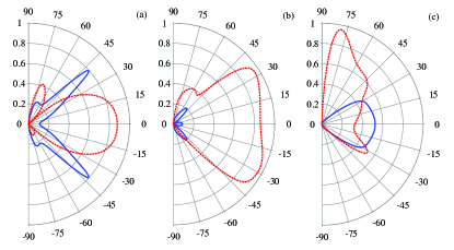
Figure 6: (Color online). Angular plot of $T_{\uparrow\uparrow}$ (solid-blue) and $T_{\downarrow\uparrow}$ (dashed-red) as a function of the injection angle for $E=2$, $\lambda=1$ and (a) $\Delta=\lambda/4$, (b) $\Delta=\lambda/2$, and $\Delta=\lambda$. The distance between the two interfaces is kept fixed to $d=\ell_{\text{SO}}$.

When only the extrinsic SOC is finite, the transmission behavior changes drastically. Two different critical angles appear — the biggest coincides usually with $\pi/2$. The extrinsic SOC induces spin precession because of the coupling between the pseudo- and the real-spin. This is illustrated in Fig. 5(b)-(c). In Panel (b) we consider the case of spin-up injection with $d=\ell_{\text{SO}}/2$. At normal incidence the transmission is entirely in the spin-down channel (dashed line). Moving away from normal incidence, the transmission in the spin-up channel (solid line) increases from zero and, after the first critical angle, the transmissions in spin-up and spin-down channels tend to coincide. In panel (c) the width of the barrier is set to $d=\ell_{\text{SO}}$. Here, the width of the SO region permits to an injected carrier at normal incidence to perform a complete precession of its spin state — the transmission is in the spin-up channel. For finite injection angles the spin-down transmission (dashed line) also becomes finite. For $\phi\lesssim\tilde{\phi}_{+}$ the transmission in the spin-up channel is almost fully suppressed while that in the spin-down channel is large. Finally, for $\phi>\tilde{\phi}_{+}$ the two transmission coefficients do not show appreciable difference.

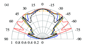
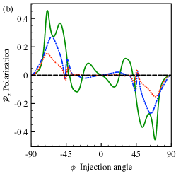
Figure 7: (Color online). Panel (a): total transmission $T$ as a function of the injection angle for $E=2$, $d=2\pi$ and several values of SOCs: $\lambda=1$ and $\Delta=0$ (blue-solid line), $\lambda=0$ and $\Delta=0.5$ (red-dotted line), $\lambda=1$ and $\Delta=\lambda/4$ (yellow-dashed line), $\Delta=\lambda/2$ (orange-dashed-dotted line), and $\lambda=\Delta$ (black-dotted-dotted-dashed line). Panel (b): $z$-component of the spin polarization ${\mathcal{P}}_{z}$ as a function on the injection angle for $E=2$ and $d=2\pi$ and the following values of the SOCs: $\lambda=1$, $\Delta=0$ and $\lambda=0$, $\Delta=1$ (same black-dashed line), $\lambda=1$ and $\Delta=\lambda/4$ (red-dotted), $\Delta=\lambda/2$ (blue-dotted-dashed line), and $\Delta=\lambda$ (green-solid line).

In the case where both extrinsic and intrinsic SOC are finite, the transmission probability exhibits a richer structure. We focus again on the case of injection of spin-up quasiparticles. Moreover we fix the width of the SO region so that it is always equal to the spin-precession length $d=\ell_{\text{SO}}$. Fig. 6 illustrates the transmission probabilities $T_{s\uparrow}$ for three values of the ratio $\Delta/\lambda=1/4,1/2,1$. Notice that from panel (a) to (c) the width of SO region decreases.

The symmetry properties of the transmission function can be rationalized by using the symmetry operation (16). Proceeding in a similar manner as in the case of the single interface, for the SO barrier we find the following symmetry relations

$$T_{s,s}(\phi) =T_{s,s}(-\phi)\,,$$ (24a)

$$T_{s,-s}(\phi) =T_{-s,s}(-\phi)\,,$$ (24b)

which are confirmed by the explicit calculations.

So far we have considered the injection of a pure spin state — the injected carrier was either in a spin-up state or a spin-down state. Following Ref. marigliano2, we now address the transmission of an unpolarized statistical mixture of spin-up and spin-down carriers. This will characterize the spin-filtering properties of the SO barrier. In the injection N region, an unpolarized statistical mixture of spins is defined by the density matrix

$$\rho_{\text{in}}=\frac{1}{2}|\chi_{\uparrow}\,\rangle\langle\,\chi_{\uparrow}|+\frac{1}{2}|\chi_{\downarrow}\,\rangle\langle\,\chi_{\downarrow}|,$$ (25)

where $|\chi_{s}\,\rangle\equiv|s\,\rangle\otimes|\sigma\,\rangle$ with $|\sigma\,\rangle=(1/\sqrt{2})(1,\text{e}^{\text{i}\phi})$ corresponds to a pure spin state. When traveling through the SO region, the injected spin-unpolarized state is subjected to spin-precession. The density matrix in the output N region can be expressed in terms of the transmission functions (19) as

$$\rho_{\text{out}}=\frac{1}{2}T_{\uparrow}|\zeta_{\uparrow}\,\rangle\langle\,\zeta_{\uparrow}|+\frac{1}{2}T_{\downarrow}|\zeta_{\downarrow}\,\rangle\langle\,\zeta_{\downarrow}|,$$ (26)

where the coefficients $T_{s}=T_{\uparrow s}+T_{\downarrow s}$ are the total transmissions for fixed injection state. The spinor part is defined as

$$|\zeta_{s}\,\rangle=\frac{1}{\sqrt{T_{s}}}\begin{pmatrix}t_{\uparrow s}\\ t_{\downarrow s}\end{pmatrix}\otimes|\sigma\,\rangle,$$ (27)

where $t_{s^{\prime},s}$ are the transmission amplitudes for incoming (resp. outgoing) spin $s$ (resp. $s^{\prime}$). The output density matrix is used to define the total transmission

$$T=\frac{T_{\uparrow}+T_{\downarrow}}{2}$$ (28)

and the expectation value of the $z$ component of the spin-polarization

$$\mathcal{P}_{z}=\frac{1}{2}\left(T_{\uparrow\uparrow}+T_{\uparrow\downarrow}-T_{\downarrow\uparrow}-T_{\downarrow\downarrow}\right)\,.$$ (29)

In Fig. 7 we report the total transmission (panel (a)) and the $z$-component of the spin-polarization (panel (b)) as a function of the injection angle for fixed energy and width of the SO region. We observe that for an unpolarized injected state the transmission probability is an even function of the injection angle $T(\phi)=T(-\phi)$. Moreover, for injection angles larger than the first critical angle $\phi>\tilde{\phi}_{+}$, the transmission has an upper bound at $T=1/2$. On the contrary $\mathcal{P}_{z}$ is an odd function of the injection angle $\mathcal{P}_{z}(\phi)=-\mathcal{P}_{z}(-\phi)$. It is zero when at least one SOC is zero. When both SOC parameters are finite $\mathcal{P}_{z}$ is finite and reaches the largest values for $\phi>\tilde{\phi}_{+}$. The maxima in this case increase as a function of the intrinsic SOC.

To experimentally observe this polarization effect the measurement should not involve an average over the angle $\phi$, which, otherwise — due to the antisymmetry of $\mathcal{P}_{z}$ — would wash out the effect. To achieve this, one could use, e.g., magnetic barriers,ale ; luca1 which are known to act as wave vector filters.

V Conclusions

In this paper we have studied the spin-resolved transmission through SO nanostructures in graphene, i.e., systems where the strength of SOCs — both intrinsic and extrinsic — is spatially modulated. We have considered the case of an interface separating a normal region from a SO region, and a barrier geometry with a region of finite SOC sandwiched between two normal regions. We have shown that — because of the lift of spin degeneracy due to the SOCs — the scattering at the single interface gives rise to spin-double refraction: a carrier injected from the normal region propagates into the SO region along two different directions as a superposition of the two available channels. The transmission into each of the two channels depends sensitively on the injection angle and on the values of SOC parameters. In the case of a SO barrier, this result can be used to select preferential directions along which the spin polarization of an initially unpolarized carrier is strongly enhanced.

We have also analyzed the edge states occurring in the single interface problem in an appropriate range of parameters. These states exist when the SOCs open a gap in the energy spectrum and correspond to the gapless edge states supported by the boundary of topological insulators.

A natural follow-up to this work would be the detailed analysis of transport properties of such SO nanostructures. From our results for the transmission probabilities, spin-resolved conductance and noise could easily be calculated by means of the Landauer-Büttiker formalism. Moreover we plan to study other geometries, as, e.g., nanostructures with a periodic modulation of SOCs. The effects of various types of impurities on the properties discussed here is yet another interesting issue to address.

We hope that our work will stimulate further theoretical and experimental investigations on spin transport properties in graphene nanostructures.

Appendix A Graphene with uniform spin-orbit interactions.

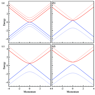
Figure 8: Spectrum of the DW Hamiltonian with intrinsic and Rashba SOC as a function of $k_{x}$ for $k_{y}=0$ . Panel (a): dashed lines refer to $\Delta=0.5$ and $\lambda=0$; solid and dotted lines refer to $\Delta=0$ and $\lambda=1$. Panel (b): $\Delta=0.4$ and $\lambda=1$. Panel (c): $\Delta=0.5$ and $\lambda=1$. Panel (d): $\Delta=0.8$ and $\lambda=1$.

In this appendix we briefly review the basic properties of DW fermions in graphene with homogeneous SO interactions.rashbagraphene The energy eigenstates are plane waves $\psi\sim\Phi({\bf k})\text{e}^{\text{i}\mathbf{k}\cdot\mathbf{r}}$ with $\Phi$ a four-component spinor and eigenvalues given by ($v_{\text{F}}=\hbar=1$)

$$E_{\alpha,\epsilon}(\mathbf{k})=\frac{\alpha\lambda}{2}+\epsilon\sqrt{k_{x}^{2}+k_{y}^{2}+\left(\Delta-\frac{\alpha\lambda}{2}\right)^{2}},$$ (30)

where $\alpha=\pm$ and $\epsilon=\pm$. The energy dispersion as a function of $k_{x}$ at fixed $k_{y}=0$ is illustrated in Fig. 8 for several values of $\Delta$ and $\lambda$. The index $\epsilon=\pm$ specifies the particle/hole branches of the spectrum. The eigenspinors $\Phi_{\alpha,\epsilon}({\bf k})$ read

$$\Phi^{\text{T}}_{\alpha,\epsilon}(\mathbf{k})= \frac{1}{2\sqrt{\cosh\theta_{\alpha}}}\times$$ (31)

$$(\text{e}^{-\text{i}\phi-\epsilon\theta_{\alpha}/2},\epsilon\text{e}^{\epsilon\theta_{\alpha}/2},\text{i}\alpha\epsilon\text{e}^{\epsilon\theta_{\alpha}/2},\text{i}\alpha\text{e}^{\text{i}\phi-\epsilon\theta_{\alpha}/2}),$$

where ${}^{\text{T}}$ denotes transposition and

$$\sinh\theta_{\alpha}=\frac{\alpha\lambda/2-\Delta}{k},$$ (32)

$$\text{e}^{\text{i}\phi}=\frac{k_{x}+\text{i}k_{y}}{k},$$ (33)

with $k=\sqrt{k_{x}^{2}+k_{y}^{2}}$. The spin operator components are expressed as $S_{j}=\frac{1}{2}s_{j}\otimes\sigma_{0}$. Their expectation values in the eigenstate $\Phi_{\alpha,\epsilon}$ read

$$\langle S_{x}\rangle =\frac{-\epsilon\alpha\sin\phi}{2\cosh\theta_{\alpha}},$$ (34a)

$$\langle S_{y}\rangle =\frac{\epsilon\alpha\cos\phi}{2\cosh\theta_{\alpha}},$$ (34b)

$$\langle S_{z}\rangle =0,$$ (34c)

which shows that the product $\epsilon\alpha$ coincides with the sign of the expectation value of the spin projection along the in plane direction perpendicular to the direction of propagation. For vanishing extrinsic SOC, the eigenstates $\Phi_{\alpha,\epsilon}$ reduce to linear combinations of eigenstates of $S_{z}$.

Similarly, the expectation value of the pseudo-spin operator $\bm{\sigma}$ is given by

$$\langle\sigma_{x}\rangle =\frac{\epsilon\cos\phi}{\cosh\theta_{\alpha}},$$ (35a)

$$\langle\sigma_{y}\rangle =\frac{\epsilon\sin\phi}{\cosh\theta_{\alpha}}.$$ (35b)

Since the SOCs in graphene do not depend on momentum, the velocity operator still coincides with the pseudo-spin operator: ${\bf v}=\dot{\bf r}=\text{i}[\mathcal{H},{\bf r}]={\bm{\sigma}}$. Thus the velocity expectation value in the state $\Phi_{\alpha,\epsilon}$ is given by Eqs. (35a–35b). Alternatively, it can be obtained from the energy dispersion as

$$\mathbf{v}_{\alpha,\epsilon}=\nabla_{\mathbf{k}}E_{\alpha,\epsilon}=\frac{\epsilon\mathbf{k}}{\sqrt{k^{2}+\left(\Delta-\frac{\alpha\lambda}{2}\right)^{2}}}\,.$$ (36)

The group velocity is then independent of the modulus of the wave vector if either the SOCs vanish or $\Delta=\alpha\lambda/2$.

References

- (1) K. S. Novoselov, A. K. Geim, S. V. Morozov, D. Jiang, Y. Zhang, S. V. Dubonos, I. V. Griegorieva, and A. A. Firsov, Science 306, 666 (2004); Nature (London) 438, 197 (2005).
- (2) Y. Zhang, Y. W. Tan, H. L. Stormer, and P. Kim, Nature (London) 438, 201 (2005).
- (3) For recent reviews, see A. K. Geim and K. S. Novoselov, Nature Mat. 6, 183 (2007); A.H. Castro Neto, F. Guinea, N. M. R. Peres, K. S. Novoselov, and A. K. Geim, Rev. Mod. Phys. 81, 109 (2009); A. K. Geim, Science 324, 1530 (2009).
- (4) C. W. J. Beenakker, Rev. Mod. Phys. 80, 1337 (2008).
- (5) G. W. Semenoff, Phys. Rev. Lett. 53, 2449 (1984).
- (6) D. P. Di Vincenzo and E.J. Mele, Phys. Rev. B 29, 1685 (1984).
- (7) I. Žutić, J. Fabian, S. Das Sarma, Rev. Mod. Phys. 76, 323 (2004).
- (8) B. Trauzettel, D.V. Bulaev, D. Loss, and G. Burkard, Nature Phys. 3, 192 (2007).
- (9) E. W. Hill, A.K.Geim, K. S. Novoselov, F. Schedin, and P. Blake, IEEE Trans. Magn. 42(10),2694 (2006).
- (10) N. Tombros, C. Jozsa, M. Popinciuc, H. T. Jonkman, and B. J. van Wees, Nature 448, 571 (2007).
- (11) S. Cho, Y.F. Chen, and M. S. Fuhrer, Appl. Phys. Lett. 91 123105 (2007).
- (12) M. Nishioka and A. M. Goldman, Appl. Phys. Lett. 90 252505 (2007).
- (13) C. Józsa, M. Popinciuc, N. Tombros, H. T. Jonkman, and B. J. van Wees, Phys. Rev. Lett. 100, 236603 (2008)
- (14) N. Tombros, S. Tanabe, A. Veligura, C. Jozsa, M. Popinciuc, H. T. Jonkman, and B. J. van Wees, Phys. Rev. Lett. 101, 046601 (2008).
- (15) C. L. Kane and E. J. Mele, Phys. Rev. Lett. 95, 226801 (2005).
- (16) D. Huertas-Hernando, F. Guinea, and A. Brataas, Phys. Rev B 74 155426 (2006).
- (17) Hongki Min, J.E. Hill, N. A. Sinitsyn, B. R. Sahu, L. Kleinman, and A.H. MacDonald, Phys. Rev. B 74, 165310 (2006).
- (18) Y. Yao, F. Ye, X. L. Qi, S. C. Zhang, and Z. Fang, Phys. Rev. B 75, 041401(R) (2007).
- (19) J. C. Boettger and S. B. Trickey, Phys. Rev. B 75, 121402(R) (2007); Phys. Rev. B 75, 199903(E) (2007).
- (20) M. Zarea and N. Sandler, Phys. Rev. B 79, 165442 (2009).
- (21) E. I. Rashba, Phys. Rev. B 79, 161409(R) (2009).
- (22) D. Huertas-Hernando, F. Guinea, and A. Brataas, Phys. Rev. Lett. 103, 146801 (2009).
- (23) C. Ertler, S. Konschuh, M. Gmitra, and J. Fabian, Phys. Rev. B 80, 041405(R) (2009).
- (24) P. Ingenhoven, J. Z. Bernád, U. Zülicke, and R. Egger Phys. Rev. B 81, 035421 (2010) .
- (25) A. Varykhalov, J. Sánchez-Barriga, A. M. Shikin, C. Biswas, E. Vescovo, A. Rybkin, D. Marchenko, and O. Rader, Phys. Rev. Lett. 101, 157601 (2008).
- (26) O. Rader, A. Varykhalov, J. Sánchez-Barriga, D. Marchenko, A. Rybkin, and A. M. Shikin, Phys. Rev. Lett. 102, 057602 (2009).
- (27) A. Varykhalov and O. Rader, Phys. Rev. B 80, 035437 (2009).
- (28) V. M. Ramaglia, D. Bercioux, V. Cataudella, G. De Filippis, C. A. Perroni, and F. Ventriglia, Eur. Phys. J. B 36, 365 (2003).
- (29) M. Khodas, A. Shekhter, and A. M. Finkel’stein, Phys. Rev. Lett. 92, 086602 (2004).
- (30) V. M. Ramaglia, D. Bercioux, V. Cataudella, G. De Filippis, and C. A. Perroni, J. Phys.: Condens. Matter 16, 9143 (2004).
- (31) E. I. Rashba, Fiz. Tverd. Tela (Leningrad) 2, 1224 (1960) [Sov. Phys. Solid State 2, 1109 (1960)].
- (32) T. Stauber and J. Schliemann, New J. Phys. 11, 115003 (2009).
- (33) A. Yamakage, K.-I. Imura, J. Cayssol, and Y. Kuramoto, EPL 87, 47005 (2009).
- (34) F. Guinea, M. I. Katsnelson, and A. G. Geim, Nature Phys. 6, 30 (2009).
- (35) B. H. J. McKellar and G. J. Stephenson, Jr., Phys. Rev. C 35, 2262 (1987).
- (36) M. Barbier, F. M. Peeters, P. Vasilopoulos, and J. M. Pereira , Phys. Rev. B 77, 115446.
- (37) L. Dell’Anna and A. De Martino, Phys. Rev. B 79, 045420 (2009); Phys. Rev. B 80, 089901(E) (2009).
- (38) L. Dell’Anna and A. De Martino, Phys. Rev. B 80, 155416 (2009).
- (39) Eigenspinors are normalized in order to ensure probability flux conservation across the interface.
-
(40)
For incidence angle larger than one of the two critical angles,
the respective refraction angle becomes complex:
where the correct determination of the imaginary part is obtained for by the relations and . - (41) F. Zhai and H. Q. Xu, Phys. Rev. Lett. 94, 246601 (2005).
- (42) A. De Martino, L. Dell’Anna, and R. Egger, Phys. Rev. Lett. 98, 066802 (2007); Sol. St. Comm. 144, 547 (2007).