Distributed coverage games for mobile visual sensor networks

Abstract

Motivated by current challenges in data-intensive sensor networks, we formulate a coverage optimization problem for mobile visual sensors as a (constrained) repeated multi-player game. Each visual sensor tries to optimize its own coverage while minimizing the processing cost. We present two distributed learning algorithms where each sensor only remembers its own utility values and actions played during the last plays. These algorithms are proven to be convergent in probability to the set of (constrained) Nash equilibria and global optima of certain coverage performance metric, respectively.

1 Introduction

There is a widespread belief that continuous and pervasive monitoring will be possible in the near future with large numbers of networked, mobile, and wireless sensors. Thus, we are witnessing an intense research activity that focuses on the design of efficient control mechanisms for these systems. In particular, decentralized algorithms would allow sensor networks to react autonomously to changes in the environment with minimal human supervision.

A substantial body of research on sensor networks has concentrated on simple sensors that can collect scalar data; e.g., temperature, humidity or pressure data. Here, a main objective is the design of algorithms that can lead to optimal collective sensing through efficient motion control and communication schemes. However, scalar measurements can be insufficient in many situations; e.g., in automated surveillance or traffic monitoring applications. In contrast, data-intensive sensors such as cameras can collect visual data that are rich in information, thus having tremendous potential for monitoring applications, but at the cost of a higher processing overhead.

Precisely, this paper aims to solve a coverage optimization problem taking into account part of the sensing/processing trade-off. Coverage optimization problems have mainly been formulated as cooperative problems where each sensor benefits from sensing the environment as a member of a group. However, sensing may also require expenditure; e.g., the energy consumed or the time spent by image processing algorithms in visual networks. Because of this, we endow each sensor with a utility function that quantifies this trade-off, formulating a coverage problem as a variation of congestion games in [26].

Literature review. In broad terms, the problem studied here is related to a bevy of sensor location and planning problems in the Computational Geometry, Geometric Optimization, and Robotics literature. For example, different variations on the (combinatorial) Art Gallery problem include [25][28][30]. The objective here is how to find the optimum number of guards in a non-convex environment so that each point is visible from at least one guard. A related set of references for the deployment of mobile robots with omnidirectional cameras includes [10][11]. Unlike the Art Gallery classic algorithms, the latter papers assume that robots have local knowledge of the environment and no recollection of the past. Other related references on robot deployment in convex environments include [6][16] for anisotropic and circular footprints.

The paper [1] is an excellent survey on multimedia sensor networks where the state of the art in algorithms, protocols, and hardware is surveyed, and open research issues are discussed in detail. As observed in [7], multimedia sensor networks enhance traditional surveillance systems by enlarging, enhancing, and enabling multi-resolution views. The investigation of coverage problems for static visual sensor networks is conducted in [5][13].

Another set of relevant references to this paper comprise those on the use of game-theoretic tools to (i) solve static target assignment problems, and (ii) devise efficient and secure algorithms for communication networks. In [18], the authors present a game-theoretic analysis of a coverage optimization problem for static sensor networks. This problem is equivalent to the weapon-target assignment problem in [24] which is nondeterministic polynomial-time complete. In general, the solution to assignment problems is hard from a combinatorial optimization viewpoint.

Game Theory and Learning in Games are used to analyze a variety of fundamental problems in; e.g., wireless communication networks and the Internet. An incomplete list of references includes [2] on power control, [27] on routing, and [29] on flow control. However, there has been limited research on how to employ Learning in Games to develop distributed algorithms for mobile sensor networks. One exception is the paper [17] where the authors establish a link between cooperative control problems (in particular, consensus problems), and games (in particular, potential games and weakly acyclic games).

Statement of contributions. The contributions of this paper pertain to both coverage optimization problems and Learning in Games. Compared with [15] and [16], this paper employs a more accurate sensing model and the results can be easily extended to include non-convex environments. Contrary to [15], we do not consider energy expenditure from sensor motions.

Regarding Learning in Games, we extend the use of the payoff-based learning dynamics in [19][20]. The coverage game we consider here is shown to be a (constrained) potential game. A number of learning rules; e.g., better (or best) reply dynamics and adaptive play, have been proposed to reach Nash equilibria in potential games. In these algorithms, each player must have access to the utility values induced by alternative actions. In our problem set-up; however, this information is unaccessible because of the information constraints caused by unknown rewards, motion and sensing limitations. To tackle this challenge, we develop two distributed payoff-based learning algorithms where each sensor only remembers its own utility values and actions played during the last plays.

In the first algorithm, at each time step, each sensor repeatedly updates its action synchronously, either trying some new action or selecting the action which corresponds to a higher utility value in the most recent two time steps. The first advantage of this algorithm over the payoff-based learning algorithms of [19][20] is its simpler dynamics, which reduces the computational complexity. Furthermore, the algorithm employs a diminishing exploration rate (in contrast to the constant one in [19][20]). The dynamically changing exploration rate renders the algorithm an inhomogeneous Markov chain (instead of the homogeneous ones in [19][20]). This technical change allows us to prove convergence in probability to the set of (constrained) Nash equilibria from which no agent is willing to unilaterally deviate. Thus, the property is substantially stronger than those in [19][20] where the algorithms are guaranteed to converge to Nash equilibria with a sufficiently large probability by choosing a sufficiently small exploration rate in advance.

The second algorithm is asynchronous. At each time step, only one sensor is active and updates its state by either trying some new action or selecting an action according to a Gibbs-like distribution from those played in last two time steps when it was active. The algorithm is shown to be convergent in probability to the set of global maxima of a coverage performance metric. Compared with the synchronous payoff-based log-linear learning algorithm in [19], this algorithm is asynchronous and simpler. Furthermore, rather than maximizing the associated potential function, the second algorithm optimizes a different global function which captures better a global trade-off between the overall network benefit from sensing and the total energy the network consumes. Again, by employing a diminishing exploration rate, our algorithm is guaranteed to have stronger convergence properties that the ones in [19].

2 Problem formulation

Here, we first review some basic game-theoretic concepts; see, for example [9]. This will allow us to formulate subsequently an optimal coverage problem for mobile visual sensor networks as a repeated multi-player game. We then introduce notation used throughout the paper.

2.1 Background in Game Theory

A strategic game $\Gamma:=\langle V,A,U\rangle$ has three components:

• A set $V$ enumerating players $i\in V:=\{1,\cdots,N\}$.

• An action set $A:=\prod_{i=1}^{N}A_{i}$ is the space of all actions vectors, where $s_{i}\in A_{i}$ is the action of player $i$ and an (multi-player) action $s\in A$ has components $s_{1},\dots,s_{N}$.

• The collection of utility functions $U$, where the utility function $u_{i}:A\rightarrow\mathbb{R}$ models player $i$’s preferences over action profiles.

Denote by $s_{-i}$ the action profile of all players other than $i$, and by $A_{-i}=\prod_{j\neq i}A_{j}$ the set of action profiles for all players except $i$. The concept of (pure) Nash equilibrium (NE, for short) is the most important one in Non-cooperative Game Theory [9] and is defined as follows.

Definition 1 (Nash equilibrium [9]).

Consider the strategic game $\Gamma$. An action profile $s^{*}:=(s_{i}^{*},s_{-i}^{*})$ is a (pure) NE of the game $\Gamma$ if $\forall i\in V$ and $\forall s_{i}\in A_{i}$, it holds that $u_{i}(s^{*})\geq u_{i}(s_{i},s_{-i}^{*})$.

An action profile corresponding to an NE represents a scenario where no player has incentive to unilaterally deviate. Potential Games form an important class of strategic games where the change in a player’s utility caused by a unilateral deviation can be measured by a potential function.

Definition 2 (Potential game [23]).

The strategic game $\Gamma$ is a potential game with potential function $\phi:A\rightarrow{\mathbb{R}}$ if for every $i\in V$, for every $s_{-i}\in A_{-i}$, and for every $s_{i},s_{i}^{\prime}\in A_{i}$, it holds that

$$\phi(s_{i},s_{-i})-\phi(s_{i}^{\prime},s_{-i})=u_{i}(s_{i},s_{-i})-u_{i}(s_{i}^{\prime},s_{-i}).$$ (1)

In conventional Non-cooperative Game Theory, all the actions in $A_{i}$ always can be selected by player $i$ in response to other players’ actions. However, in the context of motion coordination, the actions available to player $i$ will often be constrained to a state-dependent subset of $A_{i}$. In particular, we denote by $F_{i}(s_{i},s_{-i})\subseteq A_{i}$ the set of feasible actions of player $i$ when the action profile is $s:=(s_{i},s_{-i})$. We assume that $F_{i}(s_{i},s_{-i})\neq\emptyset$. Denote $F(s):=\prod_{i\in V}F_{i}(s)\subseteq A$, $\forall s\in A$ and $F:=\cup\{F(s)\;|\;s\in A\}$. The introduction of $F$ leads naturally to the notion of constrained strategic game $\Gamma_{\textup{res}}:=\langle V,A,U,F\rangle$, and the following associated concepts.

Definition 3 (Constrained Nash equilibrium).

Consider the constrained strategic game $\Gamma_{\textup{res}}$. An action profile $s^{*}$ is a constrained (pure) NE of the game $\Gamma_{\textup{res}}$ if $\forall i\in V$ and $\forall s_{i}\in F_{i}(s_{i}^{*},s_{-i}^{*})$, it holds that $u_{i}(s^{*})\geq u_{i}(s_{i},s_{-i}^{*})$.

Definition 4 (Constrained potential game).

The game $\Gamma_{\textup{res}}$ is a constrained potential game with potential function $\phi(s)$ if for every $i\in V$, every $s_{-i}\in A_{-i}$, and every $s_{i}\in A_{i}$, the equality (1) holds for every $s_{i}^{\prime}\in F_{i}(s_{i},s_{-i})$.

Observe that if $s^{*}$ is an NE of the strategic game $\Gamma$, then it is also a constrained NE of the constrained strategic game $\Gamma_{\textup{res}}$. For any given strategic game, NE may not exist. However, the existence of NE in potential games is guaranteed [23]. Hence, any constrained potential game has at least one constrained NE.

2.2 Coverage problem formulation

2.2.1 Mission space

We consider a convex 2-D mission space that is discretized into a (squared) lattice. We assume that each square of the lattice has unit dimensions. Each square will be labeled with the coordinate of its center $q=(q_{x},q_{y})$, where $q_{x}\in[q_{x_{\min}},q_{x_{\max}}]$ and $q_{y}\in[q_{y_{\min}},q_{y_{\max}}]$, for some integers $q_{x_{\min}},\;q_{y_{\min}},$ $q_{x_{\max}},\;q_{y_{\max}}$. Denote by ${\mathcal{Q}}$ the collection of all squares of the lattice.

We now define an associated location graph $\mathcal{G}_{\textup{loc}}:=({\mathcal{Q}},E_{\textup{loc}})$ where $((q_{x},q_{y}),$ $(q_{x^{\prime}},q_{y^{\prime}}))\in E_{\textup{loc}}$ if and only if $|q_{x}-q_{x^{\prime}}|+|q_{y}-q_{y^{\prime}}|=1$ for $(q_{x},q_{y}),(q_{x^{\prime}},q_{y^{\prime}})\in{\mathcal{Q}}$. Note that the graph $\mathcal{G}_{\textup{loc}}$ is undirected; i.e., $(q,q^{\prime})\in E_{\textup{loc}}$ if and only if $(q^{\prime},q)\in E_{\textup{loc}}$. The set of neighbors of $q$ in $E_{\textup{loc}}$ is given by $\mathcal{N}^{\textup{loc}}_{q}:=\{q^{\prime}\in\mathcal{Q}\setminus\{q\}\;|\;(q,q^{\prime})\in E_{\textup{loc}}\}$. We assume that the location graph ${\mathcal{G}}_{\rm loc}$ is fixed and connected, and denote its diameter by $D$.

Agents are deployed in $\mathcal{Q}$ to detect certain events of interest. As agents move in $\mathcal{Q}$ and process measurements, they will assign a numerical value $W_{q}\geq 0$ to the events in each square with center $q\in\mathcal{Q}$. If $W_{q}=0$, then there is no significant event at the square with center $q$. The larger the value of $W_{q}$ is, the more interest the set of events at the square with center $q$ is of. Later, the amount $W_{q}$ will be identified with a benefit of observing the point $q$. In this set-up, we assume the values $W_{q}$ to be constant in time. Furthermore, $W_{q}$ is not a prior knowledge to the agents, but the agents can measure this value through sensing the point $q$.

2.2.2 Modeling of the visual sensor nodes

Each mobile agent $i$ is modeled as a point mass in $\mathcal{Q}$, with location $a_{i}:=(x_{i},y_{i})\in\mathcal{Q}$. Each agent has mounted a pan-tilt-zoom camera, and can adjust its orientation and focal length.

The visual sensing range of a camera is directional, limited-range, and has a finite angle of view. Following a geometric simplification, we model the visual sensing region of agent $i$ as an annulus sector in the 2-D plane; see Figure 1.

,

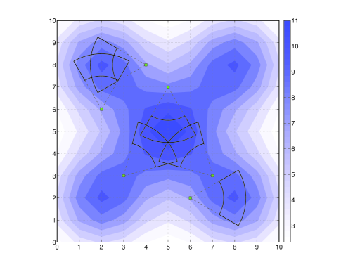
Fig. 1: Visual sensor footprint and a configuration of the mobile sensor network

The visual sensor footprint is completely characterized by the following parameters: the position of agent $i$, $a_{i}\in\mathcal{Q}$, the camera orientation, $\theta_{i}\in[0,2\pi)$, the camera angle of view, $\alpha_{i}\in[\alpha_{\textup{min}},\alpha_{\textup{max}}]$, and the shortest range (resp. longest range) between agent $i$ and the nearest (resp. farthest) object that can be recognized from the image, $r^{\textup{shrt}}_{i}\in[r_{\textup{min}},r_{\textup{max}}]$ (resp. $r^{\textup{lng}}_{i}\in[r_{\textup{min}},r_{\textup{max}}]$). The parameters $r^{\textup{shrt}}_{i}$, $r^{\textup{lng}}_{i}$, $\alpha_{i}$ can be tuned by changing the focal length $\operatorname{FL}_{i}$ of agent $i$’s camera. In this way, $c_{i}:=(\operatorname{FL}_{i},\theta_{i})\in[0,\operatorname{FL}_{\textup{max}}]\times[0,2\pi)$ is the camera control vector of agent $i$. In what follows, we will assume that $c_{i}$ takes values in a finite subset $\mathcal{C}\subset[0,\operatorname{FL}_{\textup{max}}]\times[0,2\pi)$. An agent action is thus a vector $s_{i}:=(a_{i},c_{i})\in{\mathcal{A}}_{i}:=\mathcal{Q}\times\mathcal{C}$, and a multi-agent action is denoted by $s=(s_{1},\dots,s_{N})\in\mathcal{A}:=\Pi_{i=1}^{N}\mathcal{A}_{i}$.

Let ${\mathcal{D}}(a_{i},c_{i})$ be the visual sensor footprint of agent $i$. Now we can define a proximity sensing graph $\mathcal{G}_{\textup{sen}}(s):=(V,E_{\textup{sen}}(s))$ as follows: the set of neighbors of agent $i$, $\mathcal{N}^{\textup{sen}}_{i}(s)$, is given as $\mathcal{N}^{\textup{sen}}_{i}(s):=\{j\in V\backslash\{i\}\;|\;{\mathcal{D}}(a_{i},c_{i})\cap{\mathcal{D}}(a_{j},c_{j})\cap{\mathcal{Q}}\neq\emptyset\}$.

Each agent is able to communicate with others to exchange information. We assume that the communication range of agents is $2r_{\textup{max}}$. This induces a $2r_{\textup{max}}$-disk communication graph $\mathcal{G}_{\textup{comm}}(s):=(V,E_{\textup{comm}}(s))$ as follows: the set of neighbors of agent $i$ is given by $\mathcal{N}^{\textup{comm}}_{i}(s):=\{j\in V\backslash\{i\}\;|\;(x_{i}-x_{j})^{2}+(y_{i}-y_{j})^{2}\leq(2r_{\textup{max}})^{2}\}$. Note that $\mathcal{G}_{\textup{comm}}(s)$ is undirected and that $\mathcal{G}_{\textup{sen}}(s)\subseteq\mathcal{G}_{\textup{comm}}(s)$.

The motion of agents will be limited to a neighboring point in $\mathcal{G}_{\textup{loc}}$ at each time step. Thus, an agent feasible action set will be given by ${\mathcal{F}}_{i}(a_{i}):=(\{a_{i}\}\cup\mathcal{N}^{\textup{loc}}_{a_{i}})\times{\mathcal{C}}$.

2.2.3 Coverage game

We now proceed to formulate a coverage optimization problem as a constrained strategic game. For each $q\in{\mathcal{Q}}$, we denote $n_{q}(s)$ as the cardinality of the set $\{k\in V\;|\;q\in{\mathcal{D}}(a_{k},c_{k})\cap{\mathcal{Q}}\}$; i.e., the number of agents which can observe the point $q$. The “profit” given by $W_{q}$ will be equally shared by agents that can observe the point $q$. The benefit that agent $i$ obtains through sensing is thus defined by $\sum_{q\in{\mathcal{D}}(a_{i},c_{i})\cap{\mathcal{Q}}}\frac{W_{q}}{n_{q}(s)}$.

On the other hand, and as argued in [21], the processing of visual data can incur a higher cost than that of communication. This is in contrast with scalar sensor networks, where the communication cost dominates. With this observation, we model the energy consumption of agent $i$ by $f_{i}(c_{i}):=\frac{1}{2}\alpha_{i}((r^{\textup{lng}}_{i})^{2}-(r^{\textup{shrt}}_{i})^{2})$. This measure corresponds to the area of the visual sensor footprint and can serve to approximate the energy consumption or the cost incurred by image processing algorithms.

We will endow each agent with a utility function that aims to capture the above sensing/processing trade-off. In this way, we define a utility function for agent $i$ by

$$u_{i}(s)=\sum_{q\in{\mathcal{D}}(a_{i},c_{i})\cap{\mathcal{Q}}}\frac{W_{q}}{n_{q}(s)}-f_{i}(c_{i}).$$

Note that the utility function $u_{i}$ is local over the visual sensing graph $\mathcal{G}_{\textup{sen}}(s)$; i.e., $u_{i}$ is only dependent on the actions of $\{i\}\cup\mathcal{N}^{\textup{sen}}_{i}(s)$. With the set of utility functions $U_{\textup{cov}}=\{u_{i}\}_{i\in V}$, and feasible action set $\mathcal{F}_{\textup{cov}}=\Pi_{i=1}^{N}\bigcup_{a_{i}\in\mathcal{A}_{i}}\mathcal{F}_{i}(a_{i})$, we now have all the ingredients to introduce the coverage game $\Gamma_{\textup{cov}}:=\langle V,{\mathcal{A}},U_{\textup{cov}},\mathcal{F}_{\textup{cov}}\rangle$. This game is a variation of the congestion games introduced in [26].

Lemma 5.

The coverage game $\Gamma_{\textup{cov}}$ is a constrained potential game with potential function

$$\phi(s)=\sum_{q\in{\mathcal{Q}}}\sum_{\ell=1}^{n_{q}(s)}\frac{W_{q}}{\ell}-\sum_{i=1}^{N}f_{i}(c_{i}).$$

Proof.

The proof is a slight variation of that in [26]. Consider any $s:=(s_{i},s_{-i})\in{\mathcal{A}}$ where $s_{i}:=(a_{i},c_{i})$. We fix $i\in V$ and pick any $s_{i}^{\prime}=(a_{i}^{\prime},c_{i}^{\prime})$ from ${\mathcal{F}}_{i}(a_{i})$. Denote $s^{\prime}:=(s_{i}^{\prime},s_{-i})$, $\Omega_{1}:=({\mathcal{D}}(a_{i},c_{i})\backslash{\mathcal{D}}(a_{i}^{\prime},c_{i}^{\prime}))\cap{\mathcal{Q}}$ and $\Omega_{2}:=({\mathcal{D}}(a_{i}^{\prime},c_{i}^{\prime})\backslash{\mathcal{D}}(a_{i},c_{i}))\cap{\mathcal{Q}}$. Observe that

$$\phi(s_{i},s_{-i})-\phi(s_{i}^{\prime},s_{-i})$$

$$=\sum_{q\in\Omega_{1}}(\sum_{\ell=1}^{n_{q}(s)}\frac{W_{q}}{\ell}-\sum_{\ell=1}^{n_{q}(s^{\prime})}\frac{W_{q}}{\ell})+\sum_{q\in\Omega_{2}}(-\sum_{\ell=1}^{n_{q}(s)}\frac{W_{q}}{\ell}+\sum_{\ell=1}^{n_{q}(s^{\prime})}\frac{W_{q}}{\ell})-f_{i}(c_{i})+f_{i}(c_{i}^{\prime})$$

$$=\sum_{q\in\Omega_{1}}\frac{W_{q}}{n_{q}(s)}-\sum_{q\in\Omega_{2}}\frac{W_{q}}{n_{q}(s^{\prime})}-f_{i}(c_{i})+f_{i}(c_{i}^{\prime})$$

$$=u_{i}(s_{i},s_{-i})-u_{i}(s_{i}^{\prime},s_{-i})$$

where in the second equality we utilize the fact that for each $q\in\Omega_{1}$, $n_{q}(s)=n_{q}(s^{\prime})+1$, and each $q\in\Omega_{2}$, $n_{q}(s^{\prime})=n_{q}(s)+1$. ∎

We denote by ${\mathcal{E}}(\Gamma_{\textup{cov}})$ the set of constrained NEs of $\Gamma_{\textup{cov}}$. It is worth mentioning that ${\mathcal{E}}(\Gamma_{\textup{cov}})\neq\emptyset$ due to the fact that $\Gamma_{\textup{cov}}$ is a constrained potential game.

Remark 2.1.

The assumptions of our problem formulation admit several extensions. For example, it is straightforward to extend our results to non-convex 3-D spaces. This is because the results that follow can also handle other shapes of the sensor footprint; e.g., a complete disk, a subset of the annulus sector. On the other hand, note that the coverage problem can be interpreted as a target assignment problem—here, the value $W_{q}\geq 0$ would be associated with the value of a target located at the point $q$. $\bullet$

2.3 Notations

In the following, we will use the Landau symbol, $O$, as in $O(\epsilon^{k})$, for some $k\geq 0$. This implies that $0<\lim_{\epsilon\rightarrow 0^{+}}\frac{O(\epsilon^{k})}{\epsilon^{k}}<+\infty$. We denote by $\mathop{\operator@font diag}\nolimits{\mathcal{A}}:=\{(s,s)\in{\mathcal{A}}^{2}\;|\;s\in\mathcal{A}\}$ and $\mathop{\operator@font diag}\nolimits{\mathcal{E}(\Gamma_{\textup{cov}})}:=\{(s,s)\in{\mathcal{A}}^{2}\;|\;s\in{\mathcal{E}}(\Gamma_{\rm cov})\}$.

Consider $a,a^{\prime}\in{\mathcal{Q}^{N}}$ where $a_{i}\neq a_{i}^{\prime}$ and $a_{-i}=a_{-i}^{\prime}$ for some $i\in V$. The transition $a\rightarrow a^{\prime}$ is feasible if and only if $(a_{i},a_{i}^{\prime})\in E_{\textup{loc}}$. A feasible path from $a$ to $a^{\prime}$ consisting of multiple feasible transitions is denoted by $a\Rightarrow a^{\prime}$. Let $\diamond a:=\{a^{\prime}\in\mathcal{Q}\;|\;a\Rightarrow a^{\prime}\}$ be the reachable set from $a$.

Let $s=(a,c),s^{\prime}=(a^{\prime},c^{\prime})\in{\mathcal{A}}$ where $a_{i}\neq a_{i}^{\prime}$ and $a_{-i}=a_{-i}^{\prime}$ for some $i\in V$. The transition $s\rightarrow s^{\prime}$ is feasible if and only if $s_{i}^{\prime}\in{\mathcal{F}}_{i}(a)$. A feasible path from $s$ to $s^{\prime}$ consisting of multiple feasible transitions is denoted by $s\Rightarrow s^{\prime}$. Finally, $\diamond s:=\{s^{\prime}\in{\mathcal{A}}\;|\;s\Rightarrow s^{\prime}\}$ will be the reachable set from $s$.

3 Distributed coverage learning algorithms and convergence results

In our coverage problem, we assume that $W_{q}$ is unknown in advance. Furthermore, due to the limitations of motion and sensing, each agent is unable to obtain the information of $W_{q}$ if the point $q$ is outside its sensing range. These information constraints renders that each agent is unable to access to the utility values induced by alternative actions. Thus the action-based learning algorithms; e.g., better (or best) reply learning algorithm and adaptive play learning algorithm can not be employed to solve our coverage games. It motivates us to design distributed learning algorithms which only require the payoff received.

In this section, we come up with two distributed payoff-based learning algorithms, say Distributed Inhomogeneous Synchronous Coverage Learning Algorithm ($\operatorname{DISCL}$, for short) and Distributed Inhomogeneous Asynchronous Coverage Learning Algorithm ($\operatorname{DIACL}$, for short). We then present their convergence properties. Relevant algorithms include payoff-based learning algorithms proposed in [19][20].

3.1 Distributed Inhomogeneous Synchronous Coverage Learning Algorithm

For each $t\geq 1$ and $i\in V$, we define $\tau_{i}(t)$ as follows: $\tau_{i}(t)=t$ if $u_{i}(s(t))\geq u_{i}(s(t-1))$, otherwise, $\tau_{i}(t)=t-1$. Here, $s_{i}(\tau_{i}(t))$ is the more successful action of agent $i$ in last two steps. The main steps of the $\operatorname{DISCL}$ algorithm are the following:

1:  [Initialization:] At $t=0$, all agents are uniformly placed in $\mathcal{Q}$. Each agent $i$ uniformly chooses its camera control vector $c_{i}$ from the set $\mathcal{C}$, communicates with agents in $\mathcal{N}^{\textup{sen}}_{i}(s(0))$, and computes $u_{i}(s(0))$. At $t=1$, all the agents keep their actions.

2:  [Update:] At each time $t\geq 2$, each agent $i$ updates its state according to the following rules:

• Agent $i$ chooses the exploration rate $\epsilon(t)=t^{-\frac{1}{N(D+1)}}$ and compute $s_{i}(\tau_{i}(t))$.

• With probability $\epsilon(t)$, agent $i$ experiments, and chooses the temporary action $s^{\textup{tp}}_{i}:=(a^{\textup{tp}}_{i},c^{\textup{tp}}_{i})$ uniformly from the set $\mathcal{F}_{i}(a_{i}(t))\setminus\{s_{i}(\tau_{i}(t))\}$.

• With probability $1-\epsilon(t)$, agent $i$ does not experiment, and sets $s^{\textup{tp}}_{i}=s_{i}(\tau_{i}(t))$.

• After $s^{\textup{tp}}_{i}$ is chosen, agent $i$ moves to the position $a^{\textup{tp}}_{i}$ and sets the camera control vector to $c^{\textup{tp}}_{i}$.

3:  [Communication and computation:] At position $a^{\textup{tp}}_{i}$, agent $i$ communicates with agents in $\mathcal{N}^{\textup{sen}}_{i}(s^{\textup{tp}}_{i},s^{\textup{tp}}_{-i})$, and computes $u_{i}(s^{\textup{tp}}_{i},s^{\textup{tp}}_{-i})$ and $\mathcal{F}_{i}(a^{\textup{tp}}_{i})$.

4:  Repeat Step 2 and 3.

Remark 3.1.

A variation of the $\operatorname{DISCL}$ algorithm corresponds to $\epsilon(t)=\epsilon\in(0,\frac{1}{2}]$ constant for all $t\geq 2$. If this is the case, we will refer to the algorithm as Distributed Homogeneous Synchronous Coverage Learning Algorithm ($\operatorname{DHSCL}$, for short). Later, the convergence analysis of the $\operatorname{DISCL}$ algorithm will be based on the analysis of the $\operatorname{DHSCL}$ algorithm. $\bullet$

Denote the space ${\mathcal{B}}:=\{(s,s^{\prime})\in{\mathcal{A}}\times{\mathcal{A}}\;|\;s_{i}^{\prime}\in{\mathcal{F}}_{i}(a_{i}),\;\forall i\in V\}$. Observe that $z(t):=(s(t-1),s(t))$ in the $\operatorname{DISCL}$ algorithm constitutes a time-inhomogeneous Markov chain $\{{\mathcal{P}}_{t}\}$ on the space ${\mathcal{B}}$. The following theorem states that the $\operatorname{DISCL}$ algorithm asymptotically converges to the set of $\mathcal{E}(\Gamma_{\textup{cov}})$ in probability.

Theorem 6.

Consider the Markov chain $\{{\mathcal{P}}_{t}\}$ induced by the $\operatorname{DISCL}$ Algorithm. It holds that $\lim_{t\rightarrow+\infty}{\mathbb{P}}(z(t)\in\mathop{\operator@font diag}\nolimits{\mathcal{E}(\Gamma_{\textup{cov}})})=1$.

The proofs of Theorem 6 are provided in Section 4.

Remark 3.2.

The $\operatorname{DISCL}$ algorithm is simpler than the payoff-based learning algorithm proposed in [20], reducing the computational complexity. The algorithm studied in [20] converges the set of NEs with a arbitrarily high probability by choosing a arbitrarily small exploration rate $\epsilon$ in advance. However, it is difficult to derive the relation between the convergent probability and the exploration rate. It motivates us to utilize a diminishing exploration rate in the $\operatorname{DISCL}$ algorithm which induces a time-inhomogeneous Markov chain in contrast to a time-inhomogeneous Markov chain in [20]. This change renders a stronger convergence property, i.e., the convergence to the set of NEs in probability. $\bullet$

3.2 Distributed Inhomogeneous Asynchronous Coverage Learning Algorithm

Lemma 5 shows that the coverage game $\Gamma_{\textup{cov}}$ is a constrained potential game with potential function $\phi(s)$. However, this potential function is not a straightforward measure of the network coverage performance. On the other hand, the objective function $U_{g}(s):=\sum_{i\in V}u_{i}(s)$ captures the trade-off between the overall network benefit from sensing and the total energy the network consumes, and thus can be perceived as a more natural coverage performance metric. Denote by $S^{*}:=\{s\;|\;{\rm argmax}_{s\in{\mathcal{A}}}U_{g}(s)\}$ as the set of global maximizers of $U_{g}(s)$. In this part, we present the $\operatorname{DIACL}$ algorithm which is convergent in probability to the set $S^{*}$.

Before that , we first introduce some notations for the $\operatorname{DIACL}$ algorithm. Denote by ${\mathcal{B}}^{\prime}$ the space ${{\mathcal{B}}}^{\prime}:=\{(s,s^{\prime})\in{\mathcal{A}}\times{\mathcal{A}}\;|\;s_{-i}=s_{-i}^{\prime},\;s_{i}^{\prime}\in{\mathcal{F}}_{i}(a_{i})\;{\rm for\;\;some}\;\;i\in V\}$. For any $s^{0},s^{1}\in{\mathcal{A}}$ with $s^{0}_{-i}=s^{1}_{-i}$ for some $i\in V$, we denote

$$\Delta_{i}(s^{1},s^{0}):=\frac{1}{2}\sum_{q\in\Omega_{1}}\frac{W_{q}}{n_{q}(s^{1})}-\frac{1}{2}\sum_{q\in\Omega_{2}}\frac{W_{q}}{n_{q}(s^{0})},$$

where $\Omega_{1}:={\mathcal{D}}(a_{i}^{1},c_{i}^{1})\backslash{\mathcal{D}}(a_{i}^{0},c_{i}^{0})\cap\mathcal{Q}$ and $\Omega_{2}:={\mathcal{D}}(a_{i}^{0},c_{i}^{0})\backslash{\mathcal{D}}(a_{i}^{1},c_{i}^{1})\cap\mathcal{Q}$, and

$$\rho_{i}(s^{0},s^{1}):=u_{i}(s^{1})-\Delta_{i}(s^{1},s^{0})-u_{i}(s^{0})+\Delta_{i}(s^{0},s^{1}),$$

$$\Psi_{i}(s^{0},s^{1}):=\max\{u_{i}(s^{0})-\Delta_{i}(s^{0},s^{1}),u_{i}(s^{1})-\Delta_{i}(s^{1},s^{0})\},$$

$$m^{*}:=\max_{(s^{0},s^{1})\in{\mathcal{B}},s_{i}^{0}\neq s_{i}^{1}}\{\Psi_{i}(s^{0},s^{1})-(u_{i}(s^{0})-\Delta_{i}(s^{0},s^{1})),\frac{1}{2}\}.$$

It is easy to check that $\Delta_{i}(s^{1},s^{0})=-\Delta_{i}(s^{0},s^{1})$ and $\Psi_{i}(s^{0},s^{1})=\Psi_{i}(s^{1},s^{0})$. Assume that at each time instant, one of agents becomes active with equal probability. Denote by $\gamma_{i}(t)$ the last time instant before $t$ when agent $i$ was active. We then denote $\gamma^{(2)}_{i}(t):=\gamma_{i}(\gamma_{i}(t))$. The main steps of the $\operatorname{DIACL}$ algorithm are described in the following.

1:  [Initialization:] At $t=0$, all agents are uniformly placed in $\mathcal{Q}$. Each agent $i$ uniformly chooses the camera control vector $c_{i}$ from the set $\mathcal{C}$, and then communicates with agents in $\mathcal{N}^{\textup{sen}}_{i}(s(0))$ and computes $u_{i}(s(0))$. Furthermore, each agent $i$ chooses $m_{i}\in(2m^{*},Km^{*}]$ for some $K\geq 2$. At $t=1$, all the sensors keep their actions.

2:  [Update:] Assume that agent $i$ is active at time $t\geq 2$. Then agent $i$ updates its state according to the following rules: $\bullet$ Agent $i$ chooses the exploration rate $\epsilon(t)=t^{-\frac{1}{(D+1)(K+1)m^{*}}}$. $\bullet$ With probability $\epsilon(t)^{m_{i}}$, agent $i$ experiments and uniformly chooses $s^{\textup{tp}}_{i}:=(a^{\textup{tp}}_{i},c^{\textup{tp}}_{i})$ from the action set $\mathcal{F}_{i}(a_{i}(t))\setminus\{s_{i}(t),s_{i}(\gamma_{i}^{(2)}(t)+1)\}$. $\bullet$ With probability $1-\epsilon(t)^{m_{i}}$, agent $i$ does not experiment and chooses $s^{\textup{tp}}_{i}$ according to the following probability distribution:

$$\mathbb{P}(s^{\textup{tp}}_{i}=s_{i}(t))=\frac{1}{1+\epsilon(t)^{\rho_{i}(s_{i}(\gamma_{i}^{(2)}(t)+1),s_{i}(t))}},$$

$$\mathbb{P}(s^{\textup{tp}}_{i}=s_{i}(\gamma_{i}^{(2)}(t)+1))=\frac{\epsilon(t)^{\rho_{i}(s_{i}(\gamma_{i}^{(2)}(t)+1),s_{i}(t))}}{1+\epsilon(t)^{\rho_{i}(s_{i}(\gamma_{i}^{(2)}(t)+1),s_{i}(t))}}.$$

$\bullet$ After $s^{\textup{tp}}_{i}$ is chosen, agent $i$ moves to the position $a^{\textup{tp}}_{i}$ and sets its camera control vector to be $c^{\textup{tp}}_{i}$.

3:  [Communication and computation:] At position $a^{\textup{tp}}_{i}$, the active agent $i$ communicates with agents in $\mathcal{N}^{\textup{sen}}_{i}(s^{\textup{tp}}_{i},s_{-i}(t))$, and computes $u_{i}(s^{\textup{tp}}_{i},s_{-i}(t))$, $\Delta_{i}((s^{\textup{tp}}_{i},s_{-i}(t)),s(\gamma_{i}(t)+1))$, $\mathcal{F}_{i}(a^{\textup{tp}}_{i})$.

4:  Repeat Step 2 and 3.

Remark 3.3.

A variation of the $\operatorname{DIACL}$ algorithm corresponds to $\epsilon(t)=\epsilon\in(0,\frac{1}{2}]$ constant for all $t\geq 2$. If this is the case, we will refer to the algorithm as the Distributed Homogeneous Asynchronous Coverage Learning Algorithm ($\operatorname{DHACL}$, for short). Later, we will base the convergence analysis of the $\operatorname{DIACL}$ algorithm on that of the $\operatorname{DHACL}$ algorithm. $\bullet$

Like the $\operatorname{DISCL}$ algorithm, $z(t):=(s(t-1),s(t))$ in the $\operatorname{DIACL}$ algorithm constitutes a time-inhomogeneous Markov chain $\{{\mathcal{P}}_{t}\}$ on the space ${\mathcal{B}}^{\prime}$. The following theorem states that the convergence property of the $\operatorname{DIACL}$ algorithm.

Theorem 7.

Consider the Markov chain $\{{\mathcal{P}}_{t}\}$ induced by the $\operatorname{DIACL}$ algorithm for the game $\Gamma_{\textup{cov}}$. Then it holds that $\lim_{t\rightarrow+\infty}{\mathbb{P}}(z(t)\in\mathop{\operator@font diag}\nolimits{S^{*}})=1$.

The proofs of Theorem 7 are provided in Section 4.

Remark 3.4.

The authors in [19] proposed a synchronous payoff-based log-linear learning algorithm. This algorithm is able to maximize the potential function of a potential game. While the $\operatorname{DIACL}$ algorithm is a variation of that in [19], and optimizes a different function $U_{g}(s)$. Furthermore, the convergence of the $\operatorname{DIACL}$ algorithm is in probability and stronger than the arbitrarily high probability [19] by choosing an arbitrarily small exploration rate in advance. $\bullet$

4 Convergence Analysis

In this section, we prove Theorem 6 and 7 by appealing to the Theory of Resistance Trees in [31] and the results in strong ergodicity in [14]. Relevant papers include [19][20] where the Theory of Resistance Trees in [31] is first utilized to study the class of payoff-based learning algorithms, and [12][3][22] where the strong ergodicity theory is employed to characterize the convergence properties of time-inhomogeneous Markov chains.

4.1 Convergence analysis of the $\operatorname{DISCL}$ Algorithm

We first utilize Theorem 18 to characterize the convergence properties of the associated $\operatorname{DHSCL}$ algorithm. This is essential for the analysis of the $\operatorname{DISCL}$ algorithm.

Observe that $z(t):=(s(t-1),s(t))$ in the $\operatorname{DHSCL}$ algorithm constitutes a time-homogeneous Markov chain $\{{\mathcal{P}}^{\epsilon}_{t}\}$ on the space ${\mathcal{B}}$. Consider $z,z^{\prime}\in{\mathcal{B}}$. A feasible path from $z$ to $z^{\prime}$ consisting of multiple feasible transitions of $\{{\mathcal{P}}^{\epsilon}_{t}\}$ is denoted by $z\Rightarrow z^{\prime}$. The reachable set from $z$ is denoted as $\diamond z:=\{z^{\prime}\in{\mathcal{B}}\;|\;z\Rightarrow z^{\prime}\}$.

Lemma 8.

$\{{\mathcal{P}}^{\epsilon}_{t}\}$ is a regular perturbation of $\{{\mathcal{P}}^{0}_{t}\}$.

Proof.

Consider a feasible transition $z^{1}\rightarrow z^{2}$ with $z^{1}:=(s^{0},s^{1})$ and $z^{2}:=(s^{1},s^{2})$. Then we can define a partition of $V$ as $\Lambda_{1}:=\{i\in V\;|\;s^{2}_{i}=s_{i}^{\tau_{i}(0,1)}\}$ and $\Lambda_{2}:=\{i\in V\;|\;s^{2}_{i}\in{\mathcal{F}}_{i}(a^{1}_{i})\setminus\{s^{\tau_{i}(0,1)}_{i}\}\}$. The corresponding probability is given by

$$P^{\epsilon}_{z^{1}z^{2}}=\prod_{i\in\Lambda_{1}}(1-\epsilon)\times\prod_{j\in\Lambda_{2}}\frac{\epsilon}{|\mathcal{F}_{i}(a^{1}_{i})|-1}.$$ (2)

Hence, the resistance of the transition $z^{1}\rightarrow z^{2}$ is $|\Lambda_{2}|\in\{0,1,\cdots,N\}$ since

$$0<\lim_{\epsilon\rightarrow 0^{+}}\frac{P^{\epsilon}_{z^{1}z^{2}}}{\epsilon^{|\Lambda_{2}|}}=\prod_{j\in\Lambda_{2}}\frac{1}{|\mathcal{F}_{i}(a^{1}_{i})|-1}<+\infty.$$

We have that (A3) in Section 6.2 holds. It is not difficult to see that (A2) holds, and we are now in a position to verify (A1). Since $\mathcal{G}_{\textup{loc}}$ is undirected and connected, and multiple sensors can stay in the same position, then $\diamond a^{0}={\mathcal{Q}}^{N}$ for any $a^{0}\in{\mathcal{Q}}$. Since sensor $i$ can choose any camera control vector from $\mathcal{C}$ at each time, then $\diamond s^{0}={\mathcal{A}}$ for any $s^{0}\in{\mathcal{A}}$. It implies that $\diamond z^{0}={\mathcal{B}}$ for any $z^{0}\in{\mathcal{B}}$, and thus the Markov chain $\{{\mathcal{P}}^{\epsilon}_{t}\}$ is irreducible on the space $\mathcal{B}$.

It is easy to see that any state in $\mathop{\operator@font diag}\nolimits{\mathcal{A}}$ has period $1$. Pick any $(s^{0},s^{1})\in{\mathcal{B}}\setminus\mathop{\operator@font diag}\nolimits{\mathcal{A}}$. Since $\mathcal{G}_{\textup{loc}}$ is undirected, then $s_{i}^{0}\in{\mathcal{F}}_{i}(a_{i}^{1})$ if and only if $s_{i}^{1}\in{\mathcal{F}}_{i}(a_{i}^{0})$. Hence, the following two paths are both feasible:

$$(s^{0},s^{1})\rightarrow(s^{1},s^{0})\rightarrow(s^{0},s^{1})$$

$$(s^{0},s^{1})\rightarrow(s^{1},s^{1})\rightarrow(s^{1},s^{0})\rightarrow(s^{0},s^{1}).$$

Hence, the period of the state $(s^{0},s^{1})$ is $1$. This proves aperiodicity of $\{{\mathcal{P}}^{\epsilon}_{t}\}$. Since $\{{\mathcal{P}}^{\epsilon}_{t}\}$ is irreducible and aperiodic, then (A1) holds. ∎

Lemma 9.

For any $(s^{0},s^{0})\in\mathop{\operator@font diag}\nolimits{\mathcal{A}}\setminus\mathop{\operator@font diag}\nolimits{\mathcal{E}(\Gamma_{\textup{cov}})}$, there is a finite sequence of transitions from $(s^{0},s^{0})$ to some $(s^{*},s^{*})\in\mathop{\operator@font diag}\nolimits{\mathcal{E}(\Gamma_{\textup{cov}})}$ that satisfies

$${\mathcal{L}}:=(s^{0},s^{0})\stackrel{{\scriptstyle O(\epsilon)}}{{\rightarrow}}(s^{0},s^{1})\stackrel{{\scriptstyle O(1)}}{{\rightarrow}}(s^{1},s^{1})\stackrel{{\scriptstyle O(\epsilon)}}{{\rightarrow}}(s^{1},s^{2})$$

$$\stackrel{{\scriptstyle O(1)}}{{\rightarrow}}(s^{2},s^{2})\stackrel{{\scriptstyle O(\epsilon)}}{{\rightarrow}}\cdots\stackrel{{\scriptstyle O(\epsilon)}}{{\rightarrow}}(s^{k-1},s^{k})\stackrel{{\scriptstyle O(1)}}{{\rightarrow}}(s^{k},s^{k})$$

where $(s^{k},s^{k})=(s^{*},s^{*})$ for some $k\geq 1$.

Proof.

If $s^{0}\notin{\mathcal{E}}(\Gamma_{\textup{cov}})$, there exists a sensor $i$ with a action $s_{i}^{1}\in{\mathcal{F}}_{i}(a_{i}^{0})$ such that $u_{i}(s^{1})>u_{i}(s^{0})$ where $s_{-i}^{0}=s_{-i}^{1}$. The transition $(s^{0},s^{0})\rightarrow(s^{0},s^{1})$ happens when only sensor $i$ experiments, and its corresponding probability is $(1-\epsilon)^{N-1}\times\frac{\epsilon}{|{\mathcal{F}}_{i}(a_{i}^{0})|-1}$. Since the function $\phi$ is the potential function of the game $\Gamma_{\textup{cov}}$, then we have that $\phi(s^{1})-\phi(s^{0})=u_{i}(s^{1})-u_{i}(s^{0})$ and thus $\phi(s^{1})>\phi(s^{0})$.

Since $u_{i}(s^{1})>u_{i}(s^{0})$ and $s_{-i}^{0}=s_{-i}^{1}$, the transition $(s^{0},s^{1})\rightarrow(s^{1},s^{1})$ occurs when all sensors do not experiment, and the associated probability is $(1-\epsilon)^{N}$.

We repeat the above process and construct the path $\mathcal{L}$ with length $k\geq 1$. Since $\phi(s^{i})>\phi(s^{i-1})$ for $i=\{1,\dots,k\}$, then $s^{i}\neq s^{j}$ for $i\neq j$ and thus the path $\mathcal{L}$ has no loop. Since $\mathcal{A}$ is finite, then $k$ is finite and thus $s^{k}=s^{*}\in{\mathcal{E}}(\Gamma_{\textup{cov}})$. ∎

A direct result of Lemma 8 is that for each $\epsilon$, there exists a unique stationary distribution of $\{{\mathcal{P}}^{\epsilon}_{t}\}$, say $\mu(\epsilon)$. We now proceed to utilize Theorem 18 to characterize $\lim_{\epsilon\rightarrow 0^{+}}\mu(\epsilon)$.

Proposition 10.

Consider the regular perturbation $\{{\mathcal{P}}^{\epsilon}_{t}\}$ of $\{{\mathcal{P}}^{0}_{t}\}$. Then $\displaystyle{\lim_{\epsilon\rightarrow 0^{+}}\mu(\epsilon)}$ exists and the limiting distribution $\mu(0)$ is a stationary distribution of $\{{\mathcal{P}}^{0}_{t}\}$. Furthermore, the stochastically stable states (i.e., the support of $\mu(0)$) are contained in the set $\mathop{\operator@font diag}\nolimits{\mathcal{E}(\Gamma_{\textup{cov}})}$.

Proof.

Notice that the stochastically stable states are contained in the recurrent communication classes of the unperturbed Markov chain that corresponds to the $\operatorname{DHSCL}$ Algorithm with $\epsilon=0$. Thus the stochastically stable states are included in the set $\mathop{\operator@font diag}\nolimits{\mathcal{A}}\subset{\mathcal{B}}$. Denote by $T_{\min}$ the minimum resistance tree and by $h_{v}$ the root of $T_{\min}$. Each edge of $T_{\min}$ has resistance $0,1,2,\dots$ corresponding to the transition probability $O(1),O(\epsilon),O(\epsilon^{2}),\dots$. The state $z^{\prime}$ is the $successor$ of the state $z$ if and only if $(z,z^{\prime})\in T_{\min}$. Like Theorem 3.2 in [20], our analysis will be slightly different from the presentation in 6.2. We will construct $T_{\min}$ over states in the set $\mathcal{B}$ (rather than $\mathop{\operator@font diag}\nolimits{\mathcal{A}}$) with the restriction that all the edges leaving the states in ${\mathcal{B}}\setminus\mathop{\operator@font diag}\nolimits{\mathcal{A}}$ have resistance $0$. The stochastically stable states are not changed under this difference.

Claim 1.

For any $(s^{0},s^{1})\in{\mathcal{B}}\setminus\mathop{\operator@font diag}\nolimits{\mathcal{A}}$, there is a finite path

$${\mathcal{L}}^{\prime}:=(s^{0},s^{1})\stackrel{{\scriptstyle O(1)}}{{\rightarrow}}(s^{1},s^{2})\stackrel{{\scriptstyle O(1)}}{{\rightarrow}}(s^{2},s^{2})$$

where $s_{i}^{2}=s_{i}^{\tau_{i}(0,1)}$ for all $i\in V$.

Proof.

These two transitions occur when all agents do not experiment. The corresponding probability of each transition is $(1-\epsilon)^{N}$. ∎

Claim 2.

The root $h_{v}$ belongs to the set $\mathop{\operator@font diag}\nolimits{\mathcal{A}}$.

Proof.

Suppose that $h_{v}=(s^{0},s^{1})\in{\mathcal{B}}\setminus\mathop{\operator@font diag}\nolimits{\mathcal{A}}$. By Claim 1, there is a finite path ${\mathcal{L}}^{\prime}:=(s^{0},s^{1})\stackrel{{\scriptstyle O(1)}}{{\rightarrow}}(s^{1},s^{2})\stackrel{{\scriptstyle O(1)}}{{\rightarrow}}(s^{2},s^{2})$. We now construct a new tree $T^{\prime}$ by adding the edges of the path ${\mathcal{L}}^{\prime}$ into the tree $T_{\min}$ and removing the redundant edges. The total resistance of adding edges is $0$. Observe that the resistance of the removed edge exiting from $(s^{2},s^{2})$ in the tree $T_{\min}$ is at least $1$. Hence, the resistance of $T^{\prime}$ is strictly lower than that of $T_{\min}$, and we get to a contradiction.∎

Claim 3.

Pick any ${s}^{*}\in{\mathcal{E}}(\Gamma_{\textup{cov}})$ and consider $z:=({s}^{*},{s}^{*}),$ $z^{\prime}:=({s}^{*},{\tilde{s}})$ where $\tilde{s}\neq s^{*}$. If $(z,z^{\prime})\in T_{\min}$, then the resistance of the edge $(z,z^{\prime})$ is some $k\geq 2$.

Proof.

Suppose the deviator in the transition $z\rightarrow z^{\prime}$ is unique, say $i$. Then the corresponding transition probability is $O(\epsilon)$. Since $s^{*}\in{\mathcal{E}}(\Gamma_{\textup{cov}})$ and $\tilde{s}_{i}\in{\mathcal{F}}_{i}(a_{i}^{*})$, we have that $u_{i}(s_{i}^{*},s_{-i}^{*})\geq u_{i}(\tilde{s}_{i},\tilde{s}_{-i})$, where $s_{-i}^{*}=\tilde{s}_{-i}$.

Since $z^{\prime}\in{\mathcal{B}}\setminus\mathop{\operator@font diag}\nolimits{\mathcal{A}}$, it follows from Claim 2 that the state $z^{\prime}$ can not be the root of $T_{\min}$ and thus has a successor $z^{\prime\prime}$. Note that all the edges leaving the states in ${\mathcal{B}}\setminus\mathop{\operator@font diag}\nolimits{\mathcal{A}}$ have resistance $0$. Then none experiments in the transition $z^{\prime}\rightarrow z^{\prime\prime}$ and $z^{\prime\prime}=(\tilde{s},\hat{s})$ for some $\hat{s}$. Since $u_{i}(s_{i}^{*},s_{-i}^{*})\geq u_{i}(\tilde{s}_{i},\tilde{s}_{-i})$ with $s_{-i}^{*}=\tilde{s}_{-i}$, we have $\hat{s}=s^{*}$ and thus $z^{\prime\prime}=(\tilde{s},s^{*})$. Similarly, the state $z^{\prime\prime}$ must have a successor $z^{\prime\prime\prime}$ and $z^{\prime\prime\prime}=z$. We then obtain a loop in $T_{\min}$ which contradicts that $T_{\min}$ is a tree.

It implies that at least two sensors experiment in the transition $z\rightarrow z^{\prime}$. Thus the resistance of the edge $(z,z^{\prime})$ is at least 2.∎

Claim 4.

The root $h_{v}$ belongs to the set $\mathop{\operator@font diag}\nolimits{\mathcal{E}(\Gamma_{\textup{cov}})}$.

Proof.

Suppose that $h_{v}=(s^{0},s^{0})\notin\mathop{\operator@font diag}\nolimits{\mathcal{E}(\Gamma_{\textup{cov}})}$. By Lemma 9, there is a finite path $\mathcal{L}$ connecting $(s^{0},s^{0})$ and some $(s^{*},s^{*})\in\mathop{\operator@font diag}\nolimits{\mathcal{E}(\Gamma_{\textup{cov}})}$. We now construct a new tree $T^{\prime}$ by adding the edges of the path $\mathcal{L}$ into the tree $T_{\min}$ and removing the edges that leave the states in $\mathcal{L}$ in the tree $T_{\min}$. The total resistance of adding edges is $k$. Observe that the resistance of the removed edge exiting from $(s^{i},s^{i})$ in the tree $T_{\min}$ is at least $1$ for $i\in\{1,\cdots,k-1\}$. By Claim 3, the resistance of the removed edge leaving from $(s^{*},s^{*})$ in the tree $T_{\min}$ is at least $2$. The total resistance of removing edges is at least $k+1$. Hence, the resistance of $T^{\prime}$ is strictly lower than that of $T_{\min}$, and we get to a contradiction.∎

It follows from Claim 4 that the states in $\mathop{\operator@font diag}\nolimits{\mathcal{E}(\Gamma_{\textup{cov}})}$ have minimum stochastic potential. Since Lemma 8 shows that Markov chain $\{{\mathcal{P}}^{\epsilon}_{t}\}$ is a regularly perturbed Markov process, Proposition 10 is a direct result of Theorem 18. ∎

We are now ready to show Theorem 6.

Proof of Theorem 6:

Claim 5.

Condition (B2) in Theorem 17 holds.

Proof.

For each $t\geq 0$ and each $z\in X$, we defines the numbers

$$\sigma_{z}(\epsilon(t)):=\sum_{T\in{G(z)}}\prod_{(x,y)\in T}P^{\epsilon(t)}_{xy},\quad\sigma_{z}^{t}=\sigma_{z}(\epsilon(t))$$

$$\mu_{z}(\epsilon(t)):=\frac{\sigma_{z}(\epsilon(t))}{\sum_{x\in X}\sigma_{x}(\epsilon(t))},\quad\mu_{z}^{t}=\mu_{z}(\epsilon(t)).$$

Since $\{{\mathcal{P}}^{\epsilon}_{t}\}$ is a regular perturbation of $\{{\mathcal{P}}^{0}_{t}\}$, then it is irreducible and thus $\sigma_{z}^{t}>0$. As Lemma 3.1 of Chapter 6 in [8], one can show that $(\mu^{t})^{T}P^{\epsilon(t)}=(\mu^{t})^{T}$. Therefore, condition (B2) in Theorem 17 holds.∎

Claim 6.

Condition (B3) in Theorem 17 holds.

Proof.

We now proceed to verify condition (B3) in Theorem 17. To do that, let us first fix $t$, denote $\epsilon=\epsilon(t)$ and study the monotonicity of $\mu_{z}(\epsilon)$ with respect to $\epsilon$. We write $\sigma_{z}(\epsilon)$ in the following form

$$\sigma_{z}(\epsilon)=\sum_{T\in G(z)}\prod_{(x,y)\in T}P^{\epsilon}_{xy}=\sum_{T\in G(z)}\prod_{(x,y)\in T}\frac{\alpha_{xy}(\epsilon)}{\beta_{xy}(\epsilon)}=\frac{\alpha_{z}(\epsilon)}{\beta_{z}(\epsilon)}$$ (3)

for some polynomials $\alpha_{z}(\epsilon)$ and $\beta_{z}(\epsilon)$ in $\epsilon$. With (3) in hand, we have that $\sum_{x\in X}\sigma_{x}(\epsilon)$ and thus $\mu_{z}(\epsilon)$ are ratios of two polynomials in $\epsilon$; i.e., $\mu_{z}(\epsilon)=\frac{\varphi_{z}(\epsilon)}{\beta(\epsilon)}$ where $\varphi_{z}(\epsilon)$ and $\beta(\epsilon)$ are polynomials in $\epsilon$. The derivative of $\mu_{z}(\epsilon)$ is given by

$$\frac{\partial\mu_{z}(\epsilon)}{\partial\epsilon}=\frac{1}{\beta(\epsilon)^{2}}(\frac{\partial\varphi_{z}(\epsilon)}{\partial\epsilon}\beta(\epsilon)-\varphi_{z}(\epsilon)\frac{\partial\beta(\epsilon)}{\partial\epsilon}).$$

Note that the numerator $\frac{\partial\varphi_{z}(\epsilon)}{\partial\epsilon}\beta(\epsilon)-\varphi_{z}(\epsilon)\frac{\partial\beta(\epsilon)}{\partial\epsilon}$ is a polynomial in $\epsilon$. Denote by $\iota_{z}\neq 0$ the coefficient of the leading term of $\frac{\partial\varphi_{z}(\epsilon)}{\partial\epsilon}-\varphi_{z}(\epsilon)\frac{\partial\beta(\epsilon)}{\epsilon}$. The leading term dominates $\frac{\partial\varphi_{z}(\epsilon)}{\partial\epsilon}-\varphi_{z}(\epsilon)\frac{\partial\beta(\epsilon)}{\epsilon}$ when $\epsilon$ is sufficiently small. Thus there exists $\epsilon_{z}>0$ such that the sign of $\frac{\partial\mu_{z}(\epsilon)}{\partial\epsilon}$ is the sign of $\iota_{z}$ for all $0<\epsilon\leq\epsilon_{z}$. Let $\epsilon^{*}=\max_{z\in X}\epsilon_{z}$.

Since $\epsilon(t)$ strictly decreases to zero, then there is a unique finite time instant $t^{*}$ such that $\epsilon(t^{*})=\epsilon^{*}$ (if $\epsilon(0)<\epsilon^{*}$, then $t^{*}=0$). Since $\epsilon(t)$ is strictly decreasing, we can define a partition of $X$ as follows:

$$\Xi_{1}:=\{z\in X\;|\;\mu_{z}(\epsilon(t))>\mu_{z}(\epsilon(t+1)),\quad\forall t\in[t^{*},+\infty)\},$$

$$\Xi_{2}:=\{z\in X\;|\;\mu_{z}(\epsilon(t))<\mu_{z}(\epsilon(t+1)),\quad\forall t\in[t^{*},+\infty)\}.$$

We are now ready to verify (B3) of Theorem 17. Since $\{{\mathcal{P}}^{\epsilon}_{t}\}$ is a regular perturbed Markov chain of $\{{\mathcal{P}}^{0}_{t}\}$, it follows from Theorem 18 that $\lim_{t\rightarrow+\infty}\mu_{z}(\epsilon(t))=\mu_{z}(0)$, and thus it holds that

$$\sum_{t=0}^{+\infty}\sum_{z\in X}\|\mu^{t}_{z}-\mu^{t+1}_{z}\|=\sum_{t=0}^{+\infty}\sum_{z\in X}|\mu_{z}(\epsilon(t))-\mu_{z}(\epsilon(t+1))|$$

$$=\sum_{t=0}^{t^{*}}\sum_{z\in X}|\mu_{z}(\epsilon(t))-\mu_{z}(\epsilon(t+1))|+\sum_{t=t^{*}+1}^{+\infty}(\sum_{z\in\Xi_{1}}\mu_{z}(\epsilon(t))-\sum_{z\in\Xi_{1}}\mu_{z}(\epsilon(t+1)))$$

$$+\sum_{t=t^{*}+1}^{+\infty}(1-\sum_{z\in\Xi_{1}}\mu_{z}(\epsilon(t+1))-(1-\sum_{z\in\Xi_{1}}\mu_{z}(\epsilon(t))))$$

$$=\sum_{t=0}^{t^{*}}\sum_{z\in X}|\mu_{z}(\epsilon(t))-\mu_{z}(\epsilon(t+1))|+2\sum_{z\in\Xi_{1}}\mu_{z}(\epsilon(t^{*}+1))-2\sum_{z\in\Xi_{1}}\mu_{z}(0)<+\infty.$$

∎

Claim 7.

Condition (B1) in Theorem 17 holds.

Proof.

Denote by $P^{\epsilon(t)}$ the transition matrix of $\{{\mathcal{P}}_{t}\}$. As in (2), the probability of the feasible transition $z^{1}\rightarrow z^{2}$ is given by

$$P^{\epsilon(t)}_{z^{1}z^{2}}=\prod_{i\in\Lambda_{1}}(1-\epsilon(t))\times\prod_{j\in\Lambda_{2}}\frac{\epsilon(t)}{|\mathcal{F}_{i}(a^{1}_{i})|-1}.$$

Observe that $|\mathcal{F}_{i}(a^{1}_{i})|\leq 5|{\mathcal{C}}|$. Since $\epsilon(t)$ is strictly decreasing, there is $t_{0}\geq 1$ such that $t_{0}$ is the first time when $1-\epsilon(t)\geq\frac{\epsilon(t)}{5|{\mathcal{C}}|-1}$. Then for all $t\geq t_{0}$, it holds that

$$P^{\epsilon(t)}_{z^{1}z^{2}}\geq(\frac{\epsilon(t)}{5|{\mathcal{C}}|-1})^{N}.$$

Denote $P(m,n):=\prod_{t=m}^{n-1}P^{\epsilon(t)}$, $0\leq m<n$. Pick any $z\in{\mathcal{B}}$ and let $u_{z}\in{\mathcal{B}}$ be such that $P_{u_{z}z}(t,t+D+1)=\min_{x\in{\mathcal{B}}}P_{xz}(t,t+D+1)$. Consequently, it follows that for all $t\geq t_{0}$,

$$\min_{x\in{\mathcal{B}}}P_{xz}(t,t+D+1)=\sum_{i_{1}\in{\mathcal{B}}}\cdots\sum_{i_{D}\in\in{\mathcal{B}}}P_{u_{z}i_{1}}^{\epsilon(t)}\cdots P_{i_{D-1}i_{D}}^{\epsilon(t+D-1)}P_{i_{D}z}^{\epsilon(t+D)}$$

$$\geq P_{u_{z}i_{1}}^{\epsilon(t)}\cdots P_{i_{D-1}i_{D}}^{\epsilon(t+D-1)}P_{i_{D}z}^{\epsilon(t+D)}\geq\prod_{i=0}^{D}(\frac{\epsilon(t+i)}{5|{\mathcal{C}}|-1})^{N}\geq(\frac{\epsilon(t)}{5|{\mathcal{C}}|-1})^{(D+1)N}$$

where in the last inequality we use $\epsilon(t)$ begin strictly decreasing. Then we have

$$1-\lambda(P(t,t+D+1))=\min_{x,y\in{\mathcal{B}}}\sum_{z\in{\mathcal{B}}}\min\{P_{xz}(t,t+D+1),P_{yz}(t,t+D+1)\}$$

$$\geq\sum_{z\in{\mathcal{B}}}P_{u_{z}z}(t,t+D+1)\geq|{\mathcal{B}}|(\frac{\epsilon(t)}{5|{\mathcal{C}}|-1})^{(D+1)N}.$$

Choose $k_{i}:=(D+1)i$ and let $i_{0}$ be the smallest integer such that $(D+1)i_{0}\geq t_{0}$. Then, we have that:

$$\sum_{i=0}^{+\infty}(1-\lambda(P(k_{i},k_{i+1})))\geq|{\mathcal{B}}|\sum_{i=i_{0}}^{+\infty}(\frac{\epsilon((D+1)i)}{5|{\mathcal{C}}|-1})^{(D+1)N}$$

$$=\frac{|{\mathcal{B}}|}{(5|{\mathcal{C}}|-1)^{(D+1)N}}\sum_{i=i_{0}}^{+\infty}\frac{1}{(D+1)i}=+\infty.$$ (4)

Hence, the weak ergodicity property follows from Theorem 16.∎

All the conditions in Theorem 17 hold. Thus it follows from Theorem 17 that the limiting distribution is $\mu^{*}=\lim_{t\rightarrow+\infty}\mu^{t}$. Note that $\lim_{t\rightarrow+\infty}\mu^{t}=\lim_{t\rightarrow+\infty}\mu(\epsilon(t))=\mu(0)$ and Proposition 10 shows that the support of $\mu(0)$ is contained in the set $\mathop{\operator@font diag}\nolimits{\mathcal{E}(\Gamma_{\textup{cov}})}$. Hence, the support of $\mu^{*}$ is contained in the set $\mathop{\operator@font diag}\nolimits{\mathcal{E}(\Gamma_{\textup{cov}})}$, implying that $\lim_{t\rightarrow+\infty}{\mathbb{P}}(z(t)\in\mathop{\operator@font diag}\nolimits{\mathcal{E}(\Gamma_{\textup{cov}})})=1$. This completes the proof.

4.2 Convergence analysis of the $\operatorname{DIACL}$ Algorithm

First of all, we employ Theorem 18 to study the convergence properties of the associated $\operatorname{DHACL}$ algorithm. This is essential to analyze the $\operatorname{DIACL}$ algorithm.

To simplify notations, we will use $s_{i}(t-1):=s_{i}(\gamma^{(2)}_{i}(t)+1)$ in the remainder of this section. Observe that $z(t):=(s(t-1),s(t))$ in the $\operatorname{DHACL}$ algorithm constitutes a Markov chain $\{{\mathcal{P}}^{\epsilon}_{t}\}$ on the space ${\mathcal{B}}^{\prime}$.

Lemma 11.

The Markov chain $\{{\mathcal{P}}^{\epsilon}_{t}\}$ is a regular perturbation of $\{{\mathcal{P}}^{0}_{t}\}$.

Proof.

Pick any two states $z^{1}:=(s^{0},s^{1})$ and $z^{2}:=(s^{1},s^{2})$ with $z^{1}\neq z^{2}$. We have that $P^{\epsilon}_{z^{1}z^{2}}>0$ if and only if there is some $i\in V$ such that $s_{-i}^{1}=s_{-i}^{2}$ and one of the following occurs: $s^{2}_{i}\in\mathcal{F}_{i}(a_{i}^{1})\setminus\{s^{0}_{i},s^{1}_{i}\}$, $s^{2}_{i}=s^{1}_{i}$ or $s^{2}_{i}=s^{0}_{i}$. In particular, the following holds:

$$P^{\epsilon}_{z^{1}z^{2}}=\begin{cases}\eta_{1},\quad s^{2}_{i}\in\mathcal{F}_{i}(a_{i}^{1})\setminus\{s^{0}_{i},s^{1}_{i}\},\\ \eta_{2},\quad s^{2}_{i}=s^{1}_{i},\\ \eta_{3},\quad s^{2}_{i}=s^{0}_{i},\end{cases}$$

where

$$\eta_{1}:=\frac{\epsilon^{m_{i}}}{N|\mathcal{F}_{i}(a_{i}^{1})\setminus\{s^{0}_{i},s^{1}_{i}\}|},\quad\eta_{2}:=\frac{1-\epsilon^{m_{i}}}{N(1+\epsilon^{\rho_{i}(s^{0},s^{1})})},\quad\eta_{3}:=\frac{(1-\epsilon^{m_{i}})\times\epsilon^{\rho_{i}(s^{0},s^{1})}}{N(1+\epsilon^{\rho_{i}(s^{0},s^{1})})}.$$

Observe that $0<\lim_{\epsilon\rightarrow 0^{+}}\frac{\eta_{1}}{\epsilon^{m_{i}}}<+\infty.$ Multiplying the numerator and denominator of $\eta_{2}$ by $\epsilon^{\Psi_{i}(s^{1},s^{0})-(u_{i}(s^{1})-\Delta_{i}(s^{1},s^{0}))}$, we obtain

$$\eta_{2}=\frac{1-\epsilon^{m_{i}}}{N}\times\frac{\epsilon^{\Psi_{i}(s^{0},s^{1})-(u_{i}(s^{1})-\Delta_{i}(s^{1},s^{0}))}}{\eta_{2}^{\prime}},$$

where $\eta_{2}^{\prime}:=\epsilon^{\Psi_{i}(s^{0},s^{1})-(u_{i}(s^{1})-\Delta_{i}(s^{1},s^{0}))}+\epsilon^{\Psi_{i}(s^{0},s^{1})-(u_{i}(s^{0})-\Delta_{i}(s^{0},s^{1}))}$. Use

$$\lim_{\epsilon\rightarrow 0^{+}}\epsilon^{x}=\begin{cases}1,&x=0,\\ 0,&x>0,\end{cases}$$

and we have

$$\lim_{\epsilon\rightarrow 0^{+}}\frac{\eta_{2}}{\epsilon^{\Psi_{i}(s^{0},s^{1})-(u_{i}(s^{1})-\Delta_{i}(s^{1},s^{0}))}}=\begin{cases}\frac{1}{N},&u_{i}(s^{0})-\Delta_{i}(s^{0},s^{1})\neq u_{i}(s^{1})-\Delta_{i}(s^{1},s^{0}),\\ \frac{1}{2N},&{\rm otherwise}.\end{cases}$$

Similarly, it holds that

$$\lim_{\epsilon\rightarrow 0^{+}}\frac{\eta_{3}}{\epsilon^{\Psi_{i}(s^{0},s^{1})-(u_{i}(s^{0})-\Delta_{i}(s^{0},s^{1}))}}\in\{\frac{1}{2N},\frac{1}{N}\}.$$

Hence, the resistance of the feasible transition $z^{1}\rightarrow z^{2}$, with $z^{1}\neq z^{2}$ and sensor $i$ as the unilateral deviator, can be described as follows:

$$\chi(z^{1}\rightarrow z^{2})=\begin{cases}m_{i},\quad s^{2}_{i}\in\mathcal{F}_{i}(a^{1})\setminus\{s^{0}_{i},s^{1}_{i}\},\\ \Psi_{i}(s^{0},s^{1})-(u_{i}(s^{1})-\Delta_{i}(s^{1},s^{0})),&s^{2}_{i}=s^{1}_{i},\\ \Psi_{i}(s^{0},s^{1})-(u_{i}(s^{0})-\Delta_{i}(s^{0},s^{1})),&s^{2}_{i}=s^{0}_{i}.\end{cases}$$

Then (A3) in Section 6.2 holds. It is straightforward to verify that (A2) in Section 6.2 holds. We are now in a position to verify (A1). Since $\mathcal{G}_{\textup{loc}}$ is undirected and connected, and multiple sensors can stay in the same position, then $\diamond a^{0}={\mathcal{Q}}^{N}$ for any $a^{0}\in{\mathcal{Q}}$. Since sensor $i$ can choose any camera control vector from $\mathcal{C}$ at each time, then $\diamond s^{0}={\mathcal{A}}$ for any $s^{0}\in{\mathcal{A}}$. This implies that $\diamond z^{0}={\mathcal{B}}^{\prime}$ for any $z^{0}\in{\mathcal{B}}^{\prime}$, and thus the Markov chain $\{{\mathcal{P}}^{\epsilon}_{t}\}$ is irreducible on the space ${\mathcal{B}}^{\prime}$.

It is easy to see that any state in $\mathop{\operator@font diag}\nolimits{\mathcal{A}}$ has period $1$. Pick any $(s^{0},s^{1})\in{\mathcal{B}}^{\prime}\setminus\mathop{\operator@font diag}\nolimits{\mathcal{A}}$. Since $\mathcal{G}_{\textup{loc}}$ is undirected, then $s_{i}^{0}\in{\mathcal{F}}_{i}(a_{i}^{1})$ if and only if $s_{i}^{1}\in{\mathcal{F}}_{i}(a_{i}^{0})$. Hence, the following two paths are both feasible:

$$(s^{0},s^{1})\rightarrow(s^{1},s^{0})\rightarrow(s^{0},s^{1})$$

$$(s^{0},s^{1})\rightarrow(s^{1},s^{1})\rightarrow(s^{1},s^{0})\rightarrow(s^{0},s^{1}).$$

Hence, the period of the state $(s^{0},s^{1})$ is $1$. This proves aperiodicity of $\{{\mathcal{P}}^{\epsilon}_{t}\}$. Since $\{{\mathcal{P}}^{\epsilon}_{t}\}$ is irreducible and aperiodic, then (A1) holds. ∎

A direct result of Lemma 11 is that for each $\epsilon>0$, there exists a unique stationary distribution of $\{{\mathcal{P}}^{\epsilon}_{t}\}$, say ${\mu}(\epsilon)$. From the proof of Lemma 11, we can see that the resistance of an experiment is $m_{i}$ if sensor $i$ is the unilateral deviator. We now proceed to utilize Theorem 18 to characterize $\lim_{\epsilon\rightarrow 0^{+}}{\mu}(\epsilon)$.

Proposition 12.

Consider the regular perturbed Markov process $\{{\mathcal{P}}^{\epsilon}_{t}\}$. Then $\lim_{\epsilon\rightarrow 0^{+}}{\mu}(\epsilon)$ exists and the limiting distribution ${\mu}(0)$ is a stationary distribution of $\{{\mathcal{P}}^{0}_{t}\}$. Furthermore, the stochastically stable states (i.e., the support of ${\mu}(0)$) are contained in the set $\mathop{\operator@font diag}\nolimits{S^{*}}$.

Proof.

The unperturbed Markov chain corresponds to the $\operatorname{DHACL}$ Algorithm with $\epsilon=0$. Hence, the recurrent communication classes of the unperturbed Markov chain are contained in the set $\mathop{\operator@font diag}\nolimits{\mathcal{A}}$. We will construct resistance trees over vertices in the set $\mathop{\operator@font diag}\nolimits{\mathcal{A}}$. Denote $T_{\min}$ by the minimum resistance tree. The remainder of the proof is divided into the following four claims.

Claim 8.

$\chi((s^{0},s^{0})\Rightarrow(s^{1},s^{1}))=m_{i}+\Psi_{i}(s^{1},s^{0})-(u_{i}(s^{1})-\Delta_{i}(s^{1},s^{0}))$ where $s^{0}\neq s^{1}$ and the transition $s^{0}\rightarrow s^{1}$ is feasible with sensor $i$ as the unilateral deviator.

Proof.

One feasible path for $(s^{0},s^{0})\Rightarrow(s^{1},s^{1})$ is ${\mathcal{L}}:=(s^{0},s^{0})\rightarrow(s^{0},s^{1})\rightarrow(s^{1},s^{1})$ where sensor $i$ experiments in the first transition and does not experiment in the second one. The total resistance of the path ${\mathcal{L}}$ is $m_{i}+\Psi_{i}(s^{1},s^{0})-(u_{i}(s^{1})-\Delta_{i}(s^{1},s^{0}))$ which is at most $m_{i}+m^{*}$.

Denote by ${\mathcal{L}}^{\prime}$ the path with minimum resistance among all the feasible paths for $(s^{0},s^{0})\Rightarrow(s^{1},s^{1})$. Assume that the first transition in ${\mathcal{L}}^{\prime}$ is $(s^{0},s^{0})\rightarrow(s^{0},s^{2})$ where node $j$ experiments and $s^{2}\neq s^{1}$. Observe that the resistance of $(s^{0},s^{0})\rightarrow(s^{0},s^{2})$ is $m_{j}$. No matter whether $j$ is equal to $i$ or not, the path ${\mathcal{L}}^{\prime}$ must include at least one more experiment to introduce $s_{i}^{1}$. Hence the total resistance of the path ${\mathcal{L}}^{\prime}$ is at least $m_{i}+m_{j}$. Since $m_{i}+m_{j}>m_{i}+2m^{*}$, then the path ${\mathcal{L}}^{\prime}$ has a strictly larger resistance than the path ${\mathcal{L}}$. To avoid a contradiction, the path ${\mathcal{L}}^{\prime}$ must start from the transition $(s^{0},s^{0})\rightarrow(s^{0},s^{1})$. Similarly, the sequent transition (which is also the last one) in the path ${\mathcal{L}}^{\prime}$ must be $(s^{0},s^{1})\rightarrow(s^{1},s^{1})$ and thus ${\mathcal{L}}^{\prime}={\mathcal{L}}$. Hence, the resistance of the transition $(s^{0},s^{0})\Rightarrow(s^{1},s^{1})$ is the total resistance of the path ${\mathcal{L}}$; i.e., $m_{i}+\Psi_{i}(s^{1},s^{0})-(u_{i}(s^{1})-\Delta_{i}(s^{1},s^{0}))$.∎

Claim 9.

All the edges $((s,s),(s^{\prime},s^{\prime}))$ in $T_{\min}$ must consist of only one deviator; i.e., $s_{i}\neq s_{i}^{\prime}$ and $s_{-i}=s_{-i}^{\prime}$ for some $i\in V$.

Proof.

Assume that $(s,s)\Rightarrow(s^{\prime},s^{\prime})$ has at least two deviators. Suppose the path $\hat{\mathcal{L}}$ has the minimum resistance among all the paths from $(s,s)$ to $(s^{\prime},s^{\prime})$. Then, $\ell\geq 2$ experiments are carried out along $\hat{\mathcal{L}}$. Denote $i_{k}$ by the unilateral deviator in the $k$-th experiment $s^{k-1}\rightarrow s^{k}$ where $1\leq k\leq\ell$, $s^{0}=s$ and $s^{\ell}=s^{\prime}$. Then the resistance of $\hat{\mathcal{L}}$ is at least $\sum_{k=1}^{\ell}m_{i_{k}}$; i.e., $\chi((s^{0},s^{0})\Rightarrow(s^{\prime},s^{\prime}))\geq\sum_{k=1}^{\ell}m_{i_{k}}$.

Let us consider the following path on $T_{\min}$:

$$\bar{\mathcal{L}}:=(s^{0},s^{0})\Rightarrow(s^{1},s^{1})\Rightarrow\cdots\Rightarrow(s^{\ell},s^{\ell}).$$

From Claim 1, we know that the total resistance of the path $\bar{\mathcal{L}}$ is at most $\sum_{k=1}^{\ell}m_{i_{k}}+\ell m^{*}$.

A new tree $T^{\prime}$ can be obtained by adding the edges of $\bar{\mathcal{L}}$ into $T_{\min}$ and removing the redundant edges. The removed resistance is $strictly$ greater than $\sum_{k=1}^{\ell}m_{i_{k}}+2(\ell-1)m^{*}$ where $\sum_{k=1}^{\ell}m_{i_{k}}$ is the lower bound on the resistance on the edge from $(s^{0},s^{0})$ to $(s^{\ell},s^{\ell})$, and $2(\ell-1)m^{*}$ is the strictly lower bound on the total resistances of leaving $(s^{k},s^{k})$ for $k=1,\cdots,\ell-1$. The adding resistance is the total resistance of $\bar{\mathcal{L}}$ which is at most $\sum_{k=1}^{\ell}m_{i_{k}}+\ell m^{*}$. Since $\ell\geq 2$, we have that $2(\ell-1)m^{*}\geq\ell m^{*}$ and thus $T^{\prime}$ has a strictly lower resistance than $T_{\min}$. This contradicts the fact that $T_{\min}$ is a minimum resistance tree.∎

Claim 10.

Given any edge $((s,s),(s^{\prime},s^{\prime}))$ in $T_{\min}$, denote by $i$ the unilateral deviator between $s$ and $s^{\prime}$. Then the transition $s_{i}\rightarrow s_{i}^{\prime}$ is feasible.

Proof.

Assume that the transition $s_{i}\rightarrow s_{i}^{\prime}$ is infeasible. Suppose the path $\check{\mathcal{L}}$ has the minimum resistance among all the paths from $(s,s)$ to $(s^{\prime},s^{\prime})$. Then, there are $\ell\geq 2$ experiments in $\check{\mathcal{L}}$. The remainder of the proof is similar to that of Claim 9.∎

Claim 11.

Let $h_{v}$ be the root of $T_{\min}$. Then, $h_{v}\in\mathop{\operator@font diag}\nolimits{S^{*}}$.

Proof.

Assume that $h_{v}=(s^{0},s^{0})\notin\mathop{\operator@font diag}\nolimits{S^{*}}$. Pick any $(s^{*},s^{*})\in\mathop{\operator@font diag}\nolimits{S^{*}}$. By Claim 9 and 10, we have that there is a path from $(s^{*},s^{*})$ to $(s^{0},s^{0})$ in the tree $T_{\min}$ as follows:

$$\tilde{\mathcal{L}}:=(s^{\ell},s^{\ell})\Rightarrow(s^{\ell-1},s^{\ell-1})\Rightarrow\cdots\Rightarrow(s^{1},s^{1})\Rightarrow(s^{0},s^{0})$$

for some $\ell\geq 1$. Here, $s^{*}=s^{\ell}$, there is only one deviator, say $i_{k}$, from $s^{k}$ to $s^{k-1}$, and the transition $s^{k}\rightarrow s^{k-1}$ is feasible for $k=\ell,\dots,1$.

Since the transition $s^{k}\rightarrow s^{k+1}$ is also feasible for $k=0,\dots,\ell-1$, we obtain the reverse path $\tilde{\mathcal{L}}^{\prime}$ of $\tilde{\mathcal{L}}$ as follows:

$$\tilde{\mathcal{L}}^{\prime}:=(s^{0},s^{0})\Rightarrow(s^{1},s^{1})\Rightarrow\cdots\Rightarrow(s^{\ell-1},s^{\ell-1})\Rightarrow(s^{\ell},s^{\ell}).$$

By Claim 8, the total resistance of the path $\tilde{\mathcal{L}}$ is

$$\chi({\tilde{\mathcal{L}}}) =\sum_{k=1}^{\ell}m_{i_{k}}+\sum_{k=1}^{\ell}\{\Psi_{i_{k}}(s^{k},s^{k-1})-(u_{i_{k}}(s^{k-1})-\Delta_{i_{k}}(s^{k-1},s^{k}))\},$$

and the total resistance of the path $\tilde{\mathcal{L}}^{\prime}$ is

$$\chi(\tilde{\mathcal{L}}^{\prime}) =\sum_{k=1}^{\ell}m_{i_{k}}+\sum_{k=1}^{\ell}\Psi_{i_{k}}(s^{k-1},s^{k})-(u_{i_{k}}(s^{k})-\Delta_{i_{k}}(s^{k},s^{k-1})).$$

Denote $\Lambda_{1}^{\prime}:=({\mathcal{D}}(a_{i_{k}}^{k},r_{i_{k}}^{k})\backslash{\mathcal{D}}(a_{i_{k-1}}^{k-1},r_{i_{k-1}}^{k-1}))\cap\mathcal{Q}$ and $\Lambda_{2}^{\prime}:=({\mathcal{D}}(a_{i_{k-1}}^{k-1},r_{i_{k-1}}^{k-1})\backslash{\mathcal{D}}(a_{i_{k}}^{k},r_{i_{k}}^{k}))\cap\mathcal{Q}$. Observe that

$$U_{g}(s^{k})-U_{g}(s^{k-1})$$

$$=u_{i_{k}}(s^{k})-u_{i_{k}}(s^{k-1})-\sum_{q\in\Lambda_{1}^{\prime}}W_{q}(\frac{n_{q}(s^{k-1})}{n_{q}(s^{k-1})}-\frac{n_{q}(s^{k-1})}{n_{q}(s^{k})})+\sum_{q\in\Lambda_{2}^{\prime}}W_{q}(\frac{n_{q}(s^{k})}{n_{q}(s^{k})}-\frac{n_{q}(s^{k})}{n_{q}(s^{k-1})})$$

$$=(u_{i_{k}}(s^{k})-\Delta_{i_{k}}(s^{k},s^{k-1}))-(u_{i_{k}}(s^{k-1})-\Delta_{i_{k}}(s^{k-1},s^{k})).$$

We now construct a new tree $T^{\prime}$ with the root $(s^{*},s^{*})$ by adding the edges of $\tilde{\mathcal{L}}^{\prime}$ to the tree $T_{\min}$ and removing the redundant edges $\tilde{\mathcal{L}}$. Since $\Psi_{i_{k}}(s^{k-1},s^{k})=\Psi_{i_{k}}(s^{k},s^{k-1})$, the difference in the total resistances across the trees $\chi(T^{\prime})$ and $\chi(T_{\min})$ is given by

$$\chi(T^{\prime})-\chi(T_{\min})=\chi(\tilde{\mathcal{L}}^{\prime})-\chi(\tilde{\mathcal{L}})$$

$$=\sum_{k=1}^{\ell}-(u_{i_{k}}(s^{k-1})-\Delta_{i_{k}}(s^{k-1},s^{k}))-\sum_{k=1}^{\ell}-(u_{i_{k}}(s^{k})-\Delta_{i_{k}}(s^{k},s^{k-1}))$$

$$=\sum_{k=1}^{\ell}(U_{g}(s^{k})-U_{g}(s^{k-1}))=U_{g}(s^{0})-U_{g}(s^{*})<0.$$

This contradicts that $T_{\min}$ is a minimum resistance tree.∎

It follows from Claim 4 that the state $h_{v}\in\mathop{\operator@font diag}\nolimits{S^{*}}$ has minimum stochastic potential. Then Proposition 12 is a direct result of Theorem 18. ∎

We are now ready to show Theorem 7.

Proof of Theorem 6:

Claim 12.

Condition (B2) in Theorem 17 holds.

Proof.

The proof is analogous to Claim 5.∎

Claim 13.

Condition (B3) in Theorem 17 holds.

Proof.

Denote by ${P}^{\epsilon(t)}$ the transition matrix of $\{{\mathcal{P}}_{t}\}$. Consider the feasible transition $z^{1}\rightarrow z^{2}$ with unilateral deviator $i$. The corresponding probability is given by

$$P^{\epsilon(t)}_{z^{1}z^{2}}=\begin{cases}\eta_{1},\quad s^{2}_{i}\in\mathcal{F}_{i}(a_{i}^{1})\setminus\{s^{0}_{i},s^{1}_{i}\},\\ \eta_{2},\quad s^{2}_{i}=s^{1}_{i},\\ \eta_{3},\quad s^{2}_{i}=s^{0}_{i},\end{cases}$$

where

$$\eta_{1}:=\frac{\epsilon(t)^{m_{i}}}{N|\mathcal{F}_{i}(a_{i}^{1})\setminus\{s^{0}_{i},s^{1}_{i}\}|},\quad\eta_{2}:=\frac{1-\epsilon(t)^{m_{i}}}{N(1+\epsilon(t)^{\rho_{i}(s^{0},s^{1})})},\quad\eta_{3}:=\frac{(1-\epsilon(t)^{m_{i}})\times\epsilon(t)^{\rho_{i}(s^{0},s^{1})}}{N(1+\epsilon(t)^{\rho_{i}(s^{0},s^{1})})}.$$

The remainder is analogous to Claim 6.∎

Claim 14.

Condition (B1) in Theorem 17 holds.

Proof.

Observe that $|\mathcal{F}_{i}(a_{i}^{1})|\leq 5|{\mathcal{C}}|$. Since $\epsilon(t)$ is strictly decreasing, there is $t_{0}\geq 1$ such that $t_{0}$ is the first time when $1-\epsilon(t)^{m_{i}}\geq\epsilon(t)^{m_{i}}$.

Observe that for all $t\geq 1$, it holds that

$$\eta_{1}\geq\frac{\epsilon(t)^{m_{i}}}{N(5|{\mathcal{C}}|-1)}\geq\frac{\epsilon(t)^{m_{i}+m^{*}}}{N(5|{\mathcal{C}}|-1)}.$$

Denote $b:=u_{i}(s^{1})-\Delta_{i}(s^{1},s^{0})$ and $a:=u_{i}(s^{0})-\Delta_{i}(s^{0},s^{1})$. Then $\rho_{i}(s^{0},s^{1})=b-a$. Since $b-a\leq m^{*}$, then for $t\geq t_{0}$ it holds that

$$\eta_{2}=\frac{1-\epsilon(t)^{m_{i}}}{N(1+\epsilon(t)^{b-a})}=\frac{(1-\epsilon(t)^{m_{i}})\epsilon(t)^{\max\{a,b\}-b}}{N(\epsilon(t)^{\max\{a,b\}-b}+\epsilon(t)^{\max\{a,b\}-a})}$$

$$\geq\frac{\epsilon(t)^{m_{i}}\epsilon(t)^{\max\{a,b\}-b}}{2N}\geq\frac{\epsilon(t)^{m_{i}+m^{*}}}{N(5|{\mathcal{C}}|-1)}.$$

Similarly, for $t\geq t_{0}$, it holds that

$$\eta_{3}=\frac{(1-\epsilon(t)^{m_{i}})\epsilon(t)^{\max\{a,b\}-a}}{N(\epsilon(t)^{\max\{a,b\}-b}+\epsilon(t)^{\max\{a,b\}-a})}\geq\frac{\epsilon(t)^{m_{i}+m^{*}}}{N(5|{\mathcal{C}}|-1)}.$$

Since $m_{i}\in(2m^{*},Km^{*}]$ for all $i\in V$ and $Km^{*}>1$, then for any feasible transition $z^{1}\rightarrow z^{2}$ with $z^{1}\neq z^{2}$, it holds that:

$$P^{\epsilon(t)}_{z^{1}z^{2}}\geq\frac{\epsilon(t)^{(K+1)m^{*}}}{N(5|{\mathcal{C}}|-1)}$$

for all $t\geq t_{0}$. Furthermore, for all $t\geq t_{0}$ and all $z^{1}\in\mathop{\operator@font diag}\nolimits{\mathcal{A}}$, we have that:

$$P_{z^{1}z^{1}}^{\epsilon(t)}=1-\frac{1}{N}\sum_{i=1}^{N}\epsilon(t)^{m_{i}}=\frac{1}{N}\sum_{i=1}^{N}(1-\epsilon(t)^{m_{i}})\geq\frac{1}{N}\sum_{i=1}^{N}\epsilon(t)^{m_{i}}\geq\frac{\epsilon(t)^{(K+1)m^{*}}}{N(5|{\mathcal{C}}|-1)}.$$

Choose $k_{i}:=(D+1){i}$ and let $i_{0}$ be the smallest integer such that $(D+1)i_{0}\geq t_{0}$. Similar to (4), we can derive the following property

$$\sum_{\ell=0}^{+\infty}(1-\lambda(P(k_{\ell},k_{\ell+1})))\geq\frac{|\mathcal{B}|}{(N(5|{\mathcal{C}}|-1))^{(D+1)(K+1)m^{*}}}\sum_{i=i_{0}}^{+\infty}\frac{1}{(D+1)i}=+\infty.$$

Hence, the weak ergodicity of $\{{\mathcal{P}}_{t}\}$ follows from Theorem 16.∎

All the conditions in Theorem 17 hold. Thus it follows from Theorem 17 that the limiting distribution is $\mu^{*}=\lim_{t\rightarrow+\infty}\mu^{t}$. Note that $\lim_{t\rightarrow+\infty}\mu^{t}=\lim_{t\rightarrow+\infty}\mu(\epsilon(t))=\mu(0)$ and Proposition 12 shows that the support of $\mu(0)$ is contained in the set $\mathop{\operator@font diag}\nolimits{S^{*}}$. Hence, the support of $\mu^{*}$ is contained in the set $\mathop{\operator@font diag}\nolimits{S^{*}}$, implying that $\lim_{t\rightarrow+\infty}{\mathbb{P}}(z(t)\in\mathop{\operator@font diag}\nolimits{S^{*}})=1$. It completes the proof.

5 Conclusions

We have formulated a coverage optimization problem as a constrained potential game. We have proposed two payoff-based distributed learning algorithms for this coverage game and shown that these algorithms converge in probability to the set of constrained NEs and the set of global optima of certain coverage performance metric, respectively.

6 Appendix

For the sake of a self-contained exposition, we include here some background in Markov chains [14] and the Theory of Resistance Trees [31].

6.1 Background in Markov chains

A discrete-time Markov chain is a discrete-time stochastic process on a finite (or countable) state space and satisfies the Markov property (i.e., the future state depends on its present state, but not the past states). A discrete-time Markov chain is said to be time-homogeneous if the probability of going from one state to another is independent of the time when the step is taken. Otherwise, the Markov chain is said to be time-inhomogeneous.

Since time-inhomogeneous Markov chains include time-homogeneous ones as special cases, we will restrict our attention to the former in the remainder of this section. The evolution of a time-inhomogeneous Markov chain $\{{\mathcal{P}}_{t}\}$ can described by the transition matrix $P(t)$ which gives the probability of traversing from one state to another at each time $t$.

Consider a Markov chain $\{{\mathcal{P}}_{t}\}$ with time-dependent transition matrix $P(t)$ on a finite state space $X$. Denote by $P(m,n):=\prod_{t=m}^{n-1}P(t)$, $0\leq m<n$.

Definition 13 (Strong ergodicity [14]).

The Markov chain $\{{\mathcal{P}}_{t}\}$ is strongly ergodic if there exists a stochastic vector $\mu^{*}$ such that for any distribution $\mu$ on $X$ and any $m\in{\mathbb{Z}}_{+}$, it holds that $\lim_{k\rightarrow+\infty}\mu^{T}P(m,k)=(\mu^{*})^{T}$.

Strong ergodicity of $\{{\mathcal{P}}_{t}\}$ is equivalent to $\{{\mathcal{P}}_{t}\}$ being convergent in distribution and will be employed to characterize the long-run properties of our learning algorithm. The investigation of conditions under which strong ergodicity holds is aided by the introduction of the coefficient of ergodicity and weak ergodicity defined next.

Definition 14 (Coefficient of ergodicity [14]).

For any $n\times n$ stochastic matrix $P$, its coefficient of ergodicity is defined as $\lambda(P):=1-\min_{1\leq i,j\leq n}\sum_{k=1}^{n}\min(P_{ik,}P_{jk}).$

Definition 15 (Weak ergodicity [14]).

The Markov chain $\{{\mathcal{P}}_{t}\}$ is weakly ergodic if $\forall x,y,z\in X$, $\forall m\in{\mathbb{Z}}_{+}$, it holds that $\lim_{k\rightarrow+\infty}(P_{xz}(m,k)-P_{yz}(m,k))=0$.

Weak ergodicity merely implies that $\{{\mathcal{P}}_{t}\}$ asymptotically forgets its initial state, but does not guarantee convergence. For a time-homogeneous Markov chain, there is no distinction between weak ergodicity and strong ergodicity. The following theorem provides the sufficient and necessary condition for $\{{\mathcal{P}}_{t}\}$ to be weakly ergodic.

Theorem 16 ([14]).

The Markov chain $\{{\mathcal{P}}_{t}\}$ is weakly ergodic if and only if there is a strictly increasing sequence of positive numbers $k_{i}$, $i\in{\mathbb{Z}}_{+}$ such that $\sum_{i=0}^{+\infty}(1-\lambda(P(k_{i},k_{i+1}))=+\infty.$

We are now ready to present the sufficient conditions for strong ergodicity of the Markov chain $\{{\mathcal{P}}_{t}\}$.

Theorem 17 ([14]).

A Markov chain $\{{\mathcal{P}}_{t}\}$ is strongly ergodic if the following conditions hold:

(B1) The Markov chain $\{{\mathcal{P}}_{t}\}$ is weakly ergodic.

(B2) For each $t$, there exists a stochastic vector $\mu^{t}$ on $X$ such that $\mu^{t}$ is the left eigenvector of the transition matrix $P(t)$ with eigenvalue $1$.

(B3) The eigenvectors $\mu^{t}$ in (B2) satisfy $\sum_{t=0}^{+\infty}\sum_{z\in X}|\mu^{t}_{z}-\mu^{t+1}_{z}|<+\infty$.

Moreover, if $\mu^{*}=\lim_{t\rightarrow+\infty}\mu^{t}$, then $\mu^{*}$ is the vector in Definition 13.

6.2 Background in the Theory of Resistance Trees

Let $P^{0}$ be the transition matrix of the time-homogeneous Markov chain $\{{\mathcal{P}}^{0}_{t}\}$ on a finite state space $X$. And let $P^{\epsilon}$ be the transition matrix of a perturbed Markov chain, say $\{{\mathcal{P}}^{\epsilon}_{t}\}$. With probability $1-\epsilon$, the process $\{{\mathcal{P}}^{\epsilon}_{t}\}$ evolves according to $P^{0}$, while with probability $\epsilon$, the transitions do not follow $P^{0}$.

A family of stochastic processes $\{{\mathcal{P}}^{\epsilon}_{t}\}$ is called a regular perturbation of $\{{\mathcal{P}}^{0}_{t}\}$ if the following holds $\forall x,y\in X$: (A1) For some $\varsigma>0$, the Markov chain $\{{\mathcal{P}}^{\epsilon}_{t}\}$ is irreducible and aperiodic for all $\epsilon\in(0,\varsigma]$.

(A2) $\lim_{\epsilon\rightarrow 0^{+}}P_{xy}^{\epsilon}=P_{xy}^{0}$.

(A3) If $P_{xy}^{\epsilon}>0$ for some $\epsilon$, then there exists a real number $\chi(x\rightarrow y)\geq 0$ such that $\lim_{\epsilon\rightarrow 0^{+}}P_{xy}^{\epsilon}/\epsilon^{\chi(x\rightarrow y)}\in(0,+\infty)$.

In (A3), $\chi(x\rightarrow y)$ is called the resistance of the transition from $x$ to $y$.

Let $H_{1},H_{2},\cdots,H_{J}$ be the recurrent communication classes of the Markov chain $\{{\mathcal{P}}^{0}_{t}\}$. Note that within each class $H_{\ell}$, there is a path of zero resistance from every state to every other. Given any two distinct recurrence classes $H_{\ell}$ and $H_{k}$, consider all paths which start from $H_{\ell}$ and end at $H_{k}$. Denote $\chi_{\ell k}$ by the least resistance among all such paths.

Now define a complete directed graph $\mathcal{G}$ where there is one vertex $\ell$ for each recurrent class $H_{\ell}$, and the resistance on the edge $(\ell,k)$ is $\chi_{\ell k}$. An $\ell$-tree on $\mathcal{G}$ is a spanning tree such that from every vertex $k\neq\ell$, there is a unique path from $k$ to $\ell$. Denote by $G(\ell)$ the set of all $\ell$-trees on $\mathcal{G}$. The resistance of an $\ell$-tree is the sum of the resistances of its edges. The stochastic potential of the recurrent class $H_{\ell}$ is the least resistance among all $\ell$-trees in $G(\ell)$.

Theorem 18 ([31]).

Let $\{{\mathcal{P}}^{\epsilon}_{t}\}$ be a regular perturbation of $\{{\mathcal{P}}^{0}_{t}\}$, and for each $\epsilon>0$, let $\mu(\epsilon)$ be the unique stationary distribution of $\{{\mathcal{P}}^{\epsilon}_{t}\}$. Then $\lim_{\epsilon\rightarrow 0^{+}}\mu(\epsilon)$ exists and the limiting distribution $\mu(0)$ is a stationary distribution of $\{{\mathcal{P}}^{0}_{t}\}$. The stochastically stable states (i.e., the support of $\mu(0)$) are precisely those states contained in the recurrence classes with minimum stochastic potential.

References

• [1] I.F. Akyildiz, T. Melodia, and K. Chowdhury. Wireless multimedia sensor networks: a survey. IEEE Wireless Communications Magazine, 14(6):32–39, 2007.
• [2] T. Alpcan, T. Basar, and S. Dey. A power control game based on outage probabilities for multicell wireless data networks. IEEE Transactions on Wireless Communications, 5(4):890–899, 2006.
• [3] S. Anily and A. Federgruen. Ergodicity in parametric nonstationary markov chains: an application to simulated annealing methods. Operations Research, 35(6):867–874, November 1987.
• [4] F. Bullo, J. Cortés, and S. Martínez. Distributed Control of Robotic Networks. Applied Mathematics Series. Princeton University Press, September 2008. Manuscript under contract. Available electronically at http://www.coordinationbook.info.
• [5] K.Y. Chow, K.S. Lui, and E.Y. Lam. Maximizing angle coverage in visual sensor networks. In Proc. of IEEE International Conference on Communications, pages 3516–3521, June 2007.
• [6] J. Cortés, S. Martínez, and F. Bullo. Spatially-distributed coverage optimization and control with limited-range interactions. ESAIM. Control, Optimisation & Calculus of Variations, 11:691–719, 2005.
• [7] R. Cucchiara. Multimedia surveillance systems. In Proc. of the third ACM international workshop on Video surveillance and sensor networks, pages 3–10, 2005.
• [8] M. Freidlin and A. Wentzell. Random perturbations of dynamical systems. New York: Springer Verlag, 1984.
• [9] D. Fudenberg and J. Tirole. Game theory. The MIT press, 1991.
• [10] A. Ganguli, J. Cortés, and F. Bullo. Multirobot rendezvous with visibility sensors in nonconvex environments. IEEE Transactions on Robotics, 2007. (Submitted Nov 2006) To appear.
• [11] A. Ganguli, J. Cortés, and F. Bullo. Visibility-based multi-agent deployment in orthogonal environments. In American Control Conference, pages 3426–3431, New York, July 2007.
• [12] B. Gidas. Nonstationary markov chains and convergence of the annealing algorithm. Journal of Statistical Physics, 39(1):73–131, April 1985.
• [13] E. Hörster and R. Lienhart. On the optimal placement of multiple visual sensors. In Proc. of the third ACM international workshop on Video surveillance and sensor networks, pages 111–120, 2006.
• [14] D. Isaacson and R. Madsen. Markov chains. Wiley, 1976.
• [15] A. Kwok and S. Martínez. Deployment algorithms for a power-constrained mobile sensor network. International Journal of Robust and Nonlinear Control, 2008. Submitted.
• [16] K. Laventall and J. Cortés. Coverage control by multi-robot networks with limited-range anisotropic sensory. International Journal of Control, 2009. To appear.
• [17] J. R. Marden, G. Arslan, and J. S. Shamma. Connections between cooperative control and potential games. IEEE Transactions on Systems, Man and Cybernetics, Part B: Cybernetics, 2008. submitted.
• [18] J. R. Marden and A. Wierman. Distributed welfare games. Operations Research, 2008. submitted.
• [19] J.R. Marden and J.S. Shamma. Revisiting log-linear learning : asynchrony, completeness and payoff-based omplementation. Games and Economic Behavior, 2008. submitted.
• [20] J.R. Marden, H.P. Young, G. Arslan, and J.S. Shamma. Payoff based dynamics for multi-player weakly acyclic games. SIAM Journal on Control and Optimization, 2006. submitted.
• [21] C.B. Margi, V. Petkov, K. Obraczka, and R. Manduchi. Characterizing energy consumption in a visual sensor network testbed. In Proc. of 2nd International Conference on Testbeds and Research Infrastructures for the Development of Networks and Communities, pages 332–339, March 2006.
• [22] D. Mitra, F. Romeo, and A. Sangiovanni-Vincentelli. Convergence and finite-time behavior of simulated annealing. Advances in Applied Probability, 18(3):747–771, September 1986.
• [23] D. Monderer and L. Shapley. Potential games. Games and Economic Behavior, 14:124–143, 1996.
• [24] R. A. Murphey. Target-based weapon target assignment problems. In P. M. Pardalos and L. S. Pitsoulis, editors, Nonlinear Assignment Problems: Algorithms and Applications, pages 39–53. Kluwer Academic Publishers, 1999.
• [25] J. O’Rourke. Art Gallery Theorems and Algorithms. Oxford University Press, 1987.
• [26] R.W. Rosenthal. A class of games possseeing pure strategy nash equilibria. International Journal of Game Theory, 2:65–67, 1973.
• [27] T. Roughgarden. Selfish routing and the price of anarchy. MIT press, 2005.
• [28] T. C. Shermer. Recent results in art galleries. IEEE Proceedings, 80(9):1384–1399, 1992.
• [29] A. Tang and L. Andrew. Game theory for heterogeneous flow control. In Proc. of 42nd Annual Conference on Information Sciences and Systems, pages 52–56, December 2008.
• [30] J. Urrutia. Art gallery and illumination problems. In J. R. Sack and J. Urrutia, editors, Handbook of Computational Geometry, pages 973–1027. North-Holland, 2000.
• [31] H.P. Young. The evolution of conventions. Econometrica, 61:57–84, Juanary 1993.