The origin and propagation of variability in the outflows of
long duration gamma-ray bursts

Abstract

We present the results of hydrodynamical simulations of gamma-ray burst jets propagating through their stellar progenitor material and subsequently through the surrounding circumstellar medium. We consider both jets that are injected with constant properties in the center of the star and jets injected with a variable luminosity. We show that the variability properties of the jet outside the star are a combination of the variability injected at the base of the jet and the variability caused by the jet propagation through the star. Comparing power spectra for the two cases shows that the variability injected by the engine is preserved even if the jet is heavily shocked inside the star. Such shocking produces additional variability at long time scales, of order several seconds. Within the limited number of progenitors and jets investigated, our findings suggest that the broad pulses of several seconds duration typically observed in gamma-ray bursts are due to the interaction of the jet with the progenitor, while the short-timescale variability, characterized by fluctuations on time scales of milliseconds, has to be injected at the base of the jet. Studying the properties of the fast variability in GRBs may therefore provide clues to the nature of the inner engine and the mechanisms of energy extraction from it.

1 Introduction

Gamma-ray bursts (GRBs) are extremely bright and highly variable sources of gamma-ray radiation. Their isotropic equivalent emitted energy can be as large as $10^{55}$ erg (GRB080916C; Abdo et al. 2009). GRBs last between a fraction of a second and several thousand seconds and can be divided in two classes based on their duration and spectral characteristics (Kouveliotou et al. 1993). Short bursts last less than 2 s, while long bursts last between 2 and several thousand seconds. Even though some bursts seem hard to classify within this simple scheme (e.g., GRB 060505 and GRB 060614; Fynbo et al. 2006, Gal-Yam et al. 2006, Della Valle et al. 2006; GRB 060121, de Ugarte Postigo et al. 2006) it is widely believed that a substantial fraction of, if not all, long-duration GRBs are associated with the death of massive, rapidly spinning stars (Woosley 1993; MacFadyen & Woosley 1999; Stanek et al. 2003; Hjorth et al. 2003; Woosley & Bloom 2006).

Within the overall duration of the prompt phase, fast variability is commonly observed, with the shortest spikes lasting only a fraction of a millisecond (Schaefer & Walker 1999, Walker et al. 2000). Characterizing the burst variability has proved challenging, with each GRB seeming to have its own individual pattern. This is particularly frustrating since the variability can in principle carry information on the workings of the central engine, the energy dissipation processes, and the radiation mechanisms involved in the release of the burst emission. Fenimore & Ramirez-Ruiz (1999) showed that the variability time scale of GRB light curves does not evolve from the beginning to the end of the prompt emission. Their work placed a strong constraint on the dissipation process and proved that the variability in the GRB prompt emission is not due to the interaction of the fireball with the external medium (see Dermer et al. 1999; 2000 for an alternative interpretation). Beloborodov et al. (1998, 2000) analyzed the composite power spectrum of BATSE light curves, finding that it is well described by a power-law of the shape $PDS(f)\propto f^{-5/3}$, reminiscent of the Kolmogorov spectrum of fully developed turbulence.

The discovery of the association of GRBs with massive stars puts burst variability in a new light. There are two possible sources of variability in the outflow: the engine itself (MacFadyen & Woosley 1999; Aloy et al. 2000; Ouyed et al. 2003; Proga et al. 2003; McKinney & Narayan 2007; McKinney & Blandford 2009) and the interaction of the flow with the progenitor star material (Aloy et al. 2002; Gomez & Hardee 2004; Aloy & Obergaulinger 2007; Morsony et al. 2007). How these two sources of variability combine and interact to give rise to the variability in the light curve is unknown but of fundamental importance if any conclusion is to be drawn from the temporal properties of GRB light curves.

In this paper we present the results of 2D axisymmetric simulations of the propagation of baryonic GRB jets through their progenitor star material. We show simulations in which the engine is either constant or variable and compare the structure of the jets as they emerge from the progenitor star. This paper is organized as follows: in § 2 we describe our simulations, in § 3 we describe our results, and in § 4 we discuss their potential implications.

2 The simulations and the injected variability

We present the results of four simulations, each of which has the same progenitor star and average jet properties, but with different injected luminosity histories. The first simulation has uniform injected luminosity and is analogous to that already presented in Morsony et al. (2007, hereafter MLB07) and Lazzati et al. (2009 hereafter LMB09). We call this simulation uniform. The second and third simulations (variable entropy and variable baryon load) represent an inner engine that releases a luminosity that varies in time. The time history was simulated as a random series of numbers convolved with a Gaussian, to yield a flat power spectrum (white noise) out to a cutoff at $\sim 0.1$s. This represents a randomly varying energy input, with a cutoff such that all the variability is well resolved. The energy input in a real GRB could, of course, have a different power spectrum, but for our purpose of determining how the variability is modified during propagation, this input is an adequate example. The difference between the simulation that we call variable entropy and the one that we call variable baryon load is that in the former the luminosity is varied by changing the entropy $\eta=L/\dot{m}c^{2}$ holding $\dot{m}$ constant, while in the latter the luminosity is changed by changing the baryon load ${\dot{m}}$. Finally, a simulation was run with an on-off engine with a period of 0.2s (0.1s on, 0.1s off), in which the luminosity was changed by changing the baryon load ${\dot{m}}$. We identify this last simulation as step. The represents an extreme case of strong, fast variability but on a time scale that is well resolved in our simulation. A 3s section of the injected luminosity for the four simulations is shown in Figure 1.

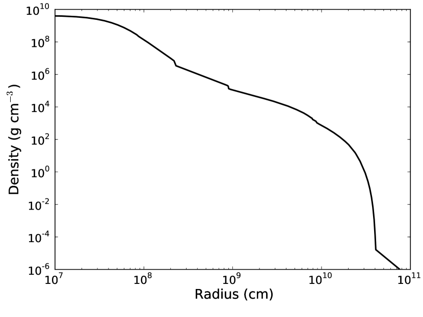
Figure 2: Density profile of the model progenitor star 16TI adopted in our simulations. From Woosley & Heger (2006).

In all simulations, the progenitor star is model 16TI from Woosley & Heger (2006, see its density profile in Fig. 2), the jet is injected at a distance $R_{0}=10^{9}$ cm from the center of the star and has an initial opening angle $\theta_{0}=10^{\circ}$ and an initial Lorentz factor $\Gamma_{0}=5$. In all simulations self-gravity is neglected, and therefore the star expands slightly under the effect of its internal pressure during the 50 seconds of our simulation. The expansion is however negligible (less then 1% of the radius) and does not affect the dynamics of the jet. In all simulations the surrounding medium is uniform, with a density $\rho=10^{-9}$ g cm${-3}$ (for the big box simulation discussed below, the density was reduced to $\rho=10^{-13}$ g cm${-3}$, LBM09). Further simulations will be performed to study the effect, if any, of a wind environment on the jet evolution outside the stellar progenitor.

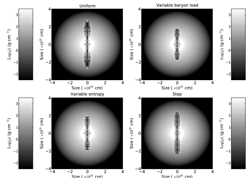
Figure 3: Density images of our four simulations 5.5 seconds after the onset of the central engine.

The simulations were performed in 2D cylindrical coordinates with the adaptive mesh refinement (AMR) special relativistic hydrodynamic code FLASH (Fryxell et al. 2000; see MLB07 for extensive testing of the special relativistic module), as modified by the authors (MLB07). The simulations were carried out for 50 seconds for a maximum number of refinements of 13 in the stellar core, corresponding to a maximum resolution of $7.8125\times 10^{6}$ cm. Outside $5\times 10^{9}$ cm from the center of the star, the maximum resolution is $3.125\times 10^{7}$ cm, corresponding to 11 levels of refinement. This is 4 times the resolution used in MLB07 and LMB09. The temporal resolution of these simulations is $1/100$th of a second. Figure 3 shows logarithmic density contours for the four simulations at $t=5.5$ s. In all panels, comoving density is shown. In all cases, a very narrow low-density jet is visible surrounded by a highly structured, turbulent cocoon of shocked stellar material.

3 Results

3.1 Effect of a variable input on the jet propagation inside the star

We first concentrate on the way in which the jets propagate through the material of their stellar progenitor. Extensive work on this topic has been done in the past (MacFadyen & Woosley 1999; Aloy et al. 2000; MacFadyen et al. 2001; Zhang et al. 2003, 2004; MLB07, Mizuta & Aloy 2009) but only in one case (Aloy et al. 2000) were variable engines considered. Aloy et al. concluded that a variable engine has a faster propagation time through the stellar progenitor.

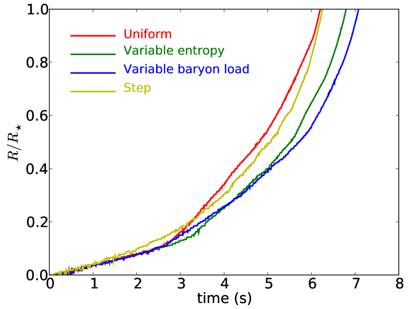
Figure 4: Propagation of the jet head through the progenitor star for the four simulations described in the text.

Figure 4 shows the propagation of the jet head through the progenitor star for our four simulations. The jet head was identified as the location of the bow shock where the outward velocity of the material exceeds 1% of the speed of light along the jet axis. Contrary to previous results, we find that the shortest propagation time is observed for a uniform injected luminosity, with the head of the jet breaking out of the star’s surface at about 6.2s, corresponding to an average velocity $v_{\rm{jh}}=0.21c$. The step simulation has a slightly longer propagation time of 6.25 s, while the variable entropy and variable baryon load simulations have longer breakout times of 6.8 and 7.1 s, respectively. It is not straightforward to understand the origin of the difference between our findings and those of Aloy et al. (2000). One possibility is that thanks to the AMR capabilities of the FLASH code, the resolution of our simulation is higher, especially as the jet approaches the stellar surface. On the other hand, Figure 4 shows that the effect of the engine variability is not simple. In the core of the star, out to approximately 20 per cent of its radius, the uniform, variable entropy, and variable baryon load jets propagate at the same speed, while the step simulation (the one most similar to the Aloy et al. 2000 set up) is ahead. At larger radii, the behaviors differentiate, with the uniform simulation showing the fastest velocity and reaching the stellar surface first. It is therefore possible that the difference between our result and the result of Aloy et al. (2000) is due to a different structure of the progenitor star. Alternatively, the difference may be due to the different prescription used in Aloy et al. (2000) for the jet injection: while we injected an outflow with net momentum as a boundary condition, Aloy et al. (2000) injected energy with no net momentum in a conical region in the core of the star , allowing a jet to develop rather than be injected. The lower boundary of the grid used by Aloy et al. (2000) is also much farther inside the star, at $2\times 10^{7}$ cm rather than $10^{9}$ cm. Differences in jet propagation may arise in this inner region that our simulations are unable to capture. Finally, it is possible that the speed of the jet head depends on the duration of the on and off phases or the frequency at which the variability is injected. The difference between our result and Aloy et al. (2000) may simply be due to the fact that we investigate variability at different frequencies.

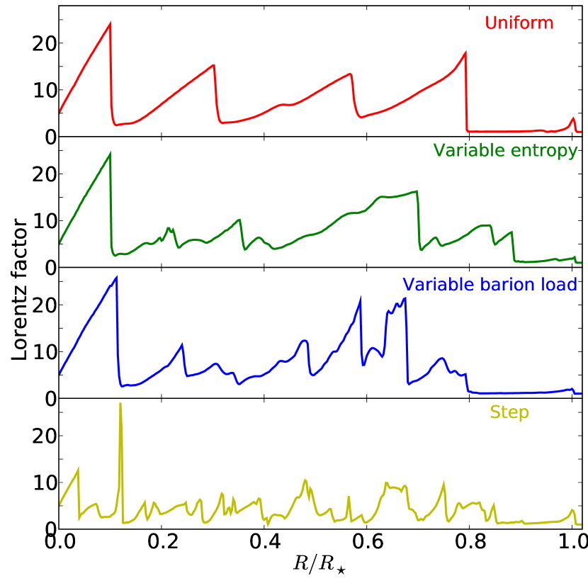
Figure 5: The dynamical conditions of the jet inside the star at the breakout time. The four panels show the Lorentz factor along the jet axis for the four simulations described in the text.

The complexity and the sensitivity to details of the interaction of the jet head with the star is also shown in Figure 5. The figure shows the Lorentz factor of the jet material along the jet axis at the moment of breakout for the four simulations. The uniform simulation has the most regular structure, with strong recollimation shocks separated by acceleration phases in which the Lorentz factor grows linearly with radius. All the variable simulations show a more complex evolution of the Lorentz factor, with milder but more numerous shocks. In particular the step simulation shows a very complex evolution of the Lorentz factor in which strong recollimation shocks are absent. This is probably due to the fact that a strong shock cannot be long lived since it is lost when it propagates from a low luminosity phase to a high luminosity one.

3.2 Variability properties of the jets outside the star

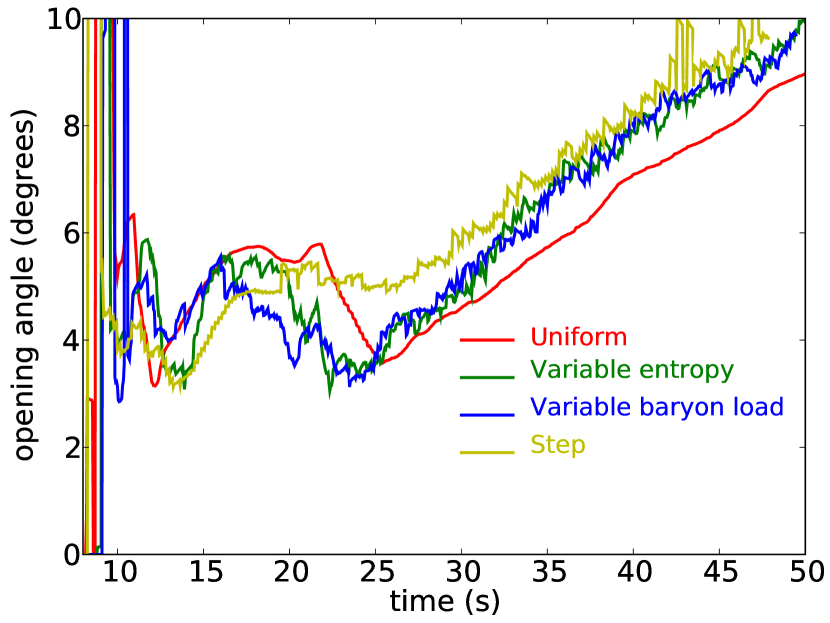
Figure 6: Jet opening angle as a function of time for the four simulations described in the text. The jet opening angle is measured at a distance of $10^{11}$ cm from the center of the progenitor star. Despite differences in the details, the variability injected by the central engine does not affect the overall evolution of the jet opening angle.

While the propagation of the jet inside the progenitor star is strongly dependent on details, the jet emerging at the surface of the star and propagating out of it is fairly insensitive to those same details. Figure 6 shows the evolution of the opening angle of the jet measured at a distance of $R=10^{11}$ cm from the center of the progenitor star (or at 2.5 stellar radii). The opening angle is measured as the geometric angle of the plasma parcel moving at $\Gamma\geq 10$ that is located farthest from the jet axis. As described in MLB07, the opening angle is initially very large, due to the quasi-isotropic cocoon material (see also Lazzati et al. 2010). Such a phase, visible in Figure 6 as the spike in angle at $t\sim 10$ s, is followed by the shocked jet phase, in which the opening angle of the jet is roughly constant and about half the size at injection. This is the phase in which the jet interaction with the progenitor star is the strongest and lasts, in all cases, approximately 10 to 15 seconds. After that, the interaction with the star becomes weak, and the jet gradually expands to its injection opening angle $\theta_{0}=10^{\circ}$. Since the jet is injected with a moderate lorentz factor $\Gamma_{0}=5$, the opening angle eventually expands to $\theta_{\rm{lim}}=\theta_{0}+1/\Gamma_{0}\sim 21\arcdeg$ (MLB07).

Even though minor differences are present, all four simulations follow the same qualitative trend, with the three phases clearly identified and lasting approximately the same time, and with approximately the same opening angle evolution. This indicates that the structure of the jet that emerges from the progenitor star is similar regardless of the short-timescale variability of the energy injection.

3.3 Light-power curves

Another way in which the structure of the jet outside the star can be investigated is through the calculation of light-power curves. The light-power curve at a radius $R$ is computed as:

$$L_{R}(t)=c\int_{\Sigma_{R}}d\sigma\left[(4p+\rho c^{2})\Gamma^{2}-\rho c^{2}\Gamma\right]\delta^{2}$$ (1)

where $\Sigma_{R}$ is a spherical surface of radius $R$ centered on the GRB engine, $p$ and $\rho$ are the pressure and comoving density of the jet, respectively, and $\delta=[\Gamma(1-\beta\cos\theta)]^{-1}$ is the Doppler factor. The luminosity in Eq. 1 is formally the luminosity that the observer would detect if all the energy were released as radiation at the radius $R$ with a 100% efficiency. The light-power curves have properties of light curves, since they contain the Doppler factor to beam photons in the direction of motion, and of power-curves, since they assume 100% efficiency and are computed at a fixed radius. In addition, we included in the computation only material that has a minimum Lorentz factor $\Gamma_{\infty,\rm{min}}=10$, since slower material is not supposed to contribute to the keV-MeV prompt light curve of GRBs.

Using the light power curve as a proxy for the light curve is a rough approximation of the processes that lead to the generation of the light curve in a GRB outflow. However, given the impossibility of following the propagation of the jet in 2D out to the radiative radius, an assumption has to be made. The rationale behind our choice is that the brightest spikes in the light curve are produced by the most energetic parts of the outflow, and the duration of a spike should be correlated to the radial thickness of the energetic part of the outflow. Such close connection is true for the photospheric scenario for the prompt emission (Rees & Meszaros 2005; LBM09) and for the internal shocks scenario, at least in first approximation (Kobayashi et al. 2007). In other words, we believe our light power curves have the right number of pulses with correct durations. If, however, we analyze the details of the light curve of individual pulses, our approximation is likely to break down, since the spectral evolution is completely missed in our approximation (see, e.g., Daigne & Mochkovitch 2002). In addition, it has been shown that second generation shells - shells produced by collisions between other shells - are complex and would produce more complex pulses than original shells (Mimica et al. 2005, 2007). So, we expect that our approximation does miss some of the fine structure in the light curves, but we also expect the overall qualitative behavior to be accurate.

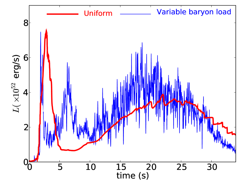
Figure 7: Comparison between the light-power curve of the uniform simulation (thick red line) and the light-power curve of the variable baryon load simulation (thin blue line). In both cases, time is measured from the instant at which relativistic matter is first detected. The two curves show analogous long-term behavior, with an initial spike followed by a broad peak lasting approximately 20 seconds. The light-power curve for the variable simulation also displays high-frequency variability at all times.

Figure 7 shows the light-power curve computed at a radius $R=2.5\times 10^{11}$ cm (the edge of our simulation box.) for the uniform and the variable baryon load simulations. Several important conclusions can be drawn from the figure. First, even if the central engine releases a constant luminosity, the power curve shows marked variability as a result of the interaction between the jet and the progenitor star. This is not a new result (MacFadyen & Woosley 1999; Aloy et al. 2000, 2002; Zhang et al. 2003, 2004; MLB07; LMB09). The comparison between the two curves shows, however, a more interesting and new conclusion. The characteristics of the long time-scale variability are similar in the two light curves, with an initial phase characterized by peaks with a width of several seconds followed by a broad bump with a duration of approximately 20 seconds. Some differences are however apparent, with a second peak appearing in the variable baryon load light power curve that is not observed in the uniform simulation.

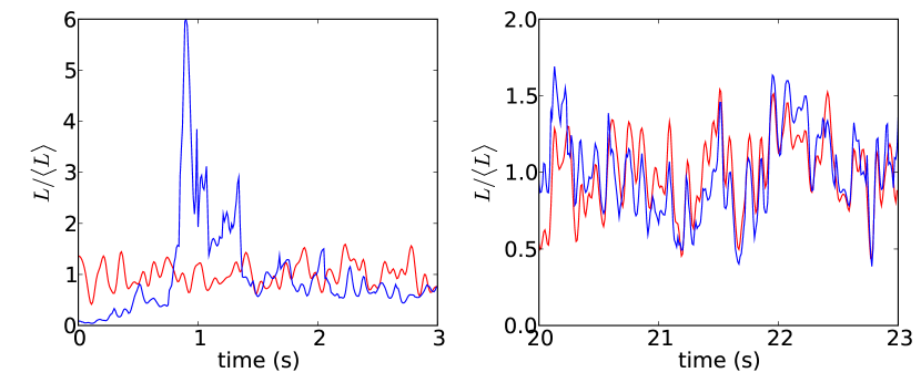
Figure 8: Comparison between the variability injected by the inner engine (red line) and the one observed in the power curve at a radius of $R=2.5\times 10^{11}$ cm. The left panel shows the initial 3 seconds of the light-power curve, while the right panel shows a central section of 3 seconds, during a phase in which the light curve is still deeply affected by the jet interaction with the progenitor star (cfr. Figure 7). While the variability of the two curves in the left panel is almost uncorrelated, a strong correlation is observed in the right panel.

Another interesting comparison is presented in Figure 8, which shows the luminosity injected at the base of the jet (red line) compared to the light-power curve measured well outside the star at radius $R=2.5\times 10^{11}$ cm for the same variable baryon load simulations shown in Fig. 7. The injected curve has been shifted in time by adding the light propagation time from the inner boundary of the simulation out to the radius at which the light power curves have been computed. In this way, the jet propagation time was removed. The left panel shows the comparison during the first three seconds of the light-power curve while the right panel shows the same comparison at a later time, still during the shocked jet phase (according to the definition of MLB07). In the left panel, fast variability is observed in the light-power curve, but it is almost completely uncorrelated with the injected variability at the base of the jet. On the other hand, at the later time shown in the right panel, the variability of the engine and that observed in the light-power curve are almost identical. A further analysis shows that the strong correlation appears at about $\sim 4$ s from the trigger and lasts until $t=30$ s, the beginning of the unshocked jet phase (MLB07). The same analysis was performed with the variable entropy and the step simulations. We found that in both cases the strong correlation is observed. However, the variable entropy light power curve is sometimes shifted in time, likely due to different propagation times of shells with different entropy and therefore different asymptotic Lorentz factor. In the step simulations, instead, the strong correlation is observed at all times, likely due to the unphysically strong character of the fluctuations injected in that model.

This suggests that there are two sub-phases within the shocked-jet phase. An initial short phase, lasting a few seconds, has the capability of modifying the variability injected by the inner engine, while a second phase, lasting several tens of seconds until the end of the shocked-jet phase, leaves the engine variability unaffected. A closer inspection of our simulations reveals that the initial short phase is characterized by perpendicular shocks, propagating along the jet similarly to internal shocks, while the latter phase is characterized by tangential shocks that propagate from the sides to the jet axis and vice versa. The fact that the variability injected by the central engine is preserved during the shocked jet phase comes as a surprise. Both Zhang et al. (2003) and MLB07 had predicted, based on simulations of constant engines, that the variability injected by the central engine, if any, would have been visible only “at very late times when the star has exploded” (Zhang et al. 2003). We find here, from the analysis of a simulation with a variable inner engine, that the transverse collimation shocks are not able to erase the short-timescale (fraction of a second) variability injected at the base of the jet by the inner engine. This finding makes us much more optimistic that the characteristics of the central engine can be studied by observing the light curves of GRBs. Further analysis is however needed to confirm the robustness of this result for different progenitors, injected luminosities, and jet properties.

The inner engine variability is also visible during the unshocked jet phase, as described in MLB07. This final phase, however, is much dimmer than the shocked jet phase and it is unclear whether it could be observed at all in GRB light curves.

3.4 Polar jet structure

The computation of light-power curves allows us to compare the amount of energy and the peak luminosity as a function of the off-axis angle $\theta_{o}$. Previous studies on the distribution of energy in the fireball with respect to $\theta_{o}$ have resulted in controversial results. Zhang et al. (2004) found a somewhat universal slope $dE/d\Omega\propto\theta^{-3}$, while MLB07 and Mizuta & Aloy (2009) found that the slope depends on the properties of the stellar progenitor, and on the limiting Lorentz factor $\Gamma_{\rm{min}}$ that is adopted. In this paper, we compute the value of $dE/d\Omega$ from the light-power curves, rather than computing it locally from the kinetic energy in the flow. As a result, the values of $dE/d\Omega$ that we obtain are smoother than those in MLB07 because they include contributions from material pointing in different directions with respect to the line of sight. This is similar to the method used in Mizuta & Aloy (2009) for including contributions from material away from the line of sight.

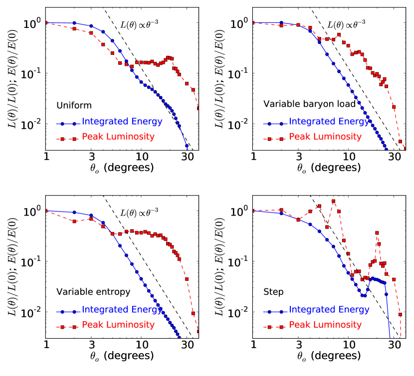
Figure 9: Angular distribution of the peak luminosity (red dashed line) and time integrated energy (blue solid line) measured in the light-power curve at $R=2.5\times 10^{11}$ cm.

Each panel of Figure 9 shows the results from one of our simulations. We find that the isotropic equivalent energy distribution $dE/d\Omega$ drops with angle smoothly in all cases, with a slope well represented by a $\theta^{-3}$ power-law, analogously to that found by Zhang et al. (2004). Only for the step simulation, a deviation is observed at $\theta_{o}\sim 20^{\circ}$ off-axis. Mizuta & Aloy (2009) found that the slope ranges from -2.7 for high mass progenitors to -3.7 for low mass progenitors. However, the progenitor model in their paper most similar to the model we use is model 16OC (from Woosley & Heger 2006). For this model, Mizuta & Aloy (2009) find a slope of -2.95, consistent with our results.

Figure 9 also shows the isotropic equivalent peak luminosity distribution $dL_{\rm{pk}}/d\Omega$, characterized by a much more varied behavior. At angles less than $\theta_{o}\sim 5^{\circ}$, the peak light-power curve tracks the isotropic equivalent energy curve. At larger angles, however, it becomes roughly constant, while the isotropic equivalent energy keeps dropping. The peak luminosity remains constant out to an angle that depends on the simulation, but is roughly a few tens of degrees; it eventually drops for very large off-axis angles.

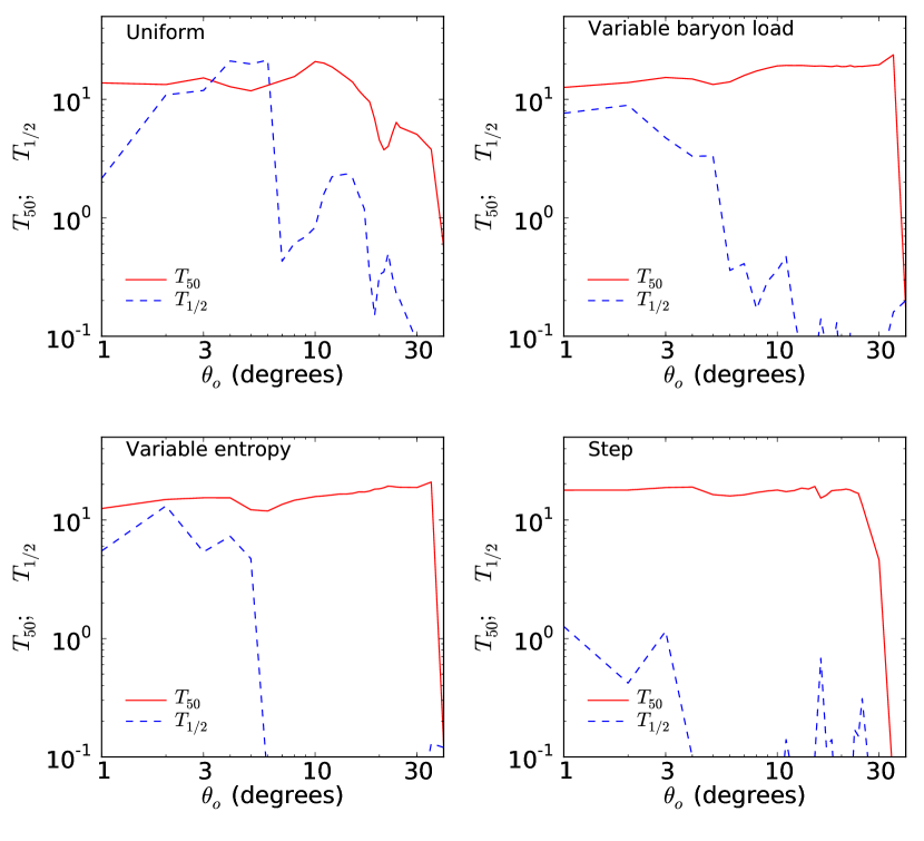
Figure 10: Duration of the synthetic GRBs as a function of the viewing geometry. The solid (dashed) line shows $T_{\rm{50}}$ ($T_{1/2}$), where $T_{50}$ is the time during which 50% of the total energy is observed, while $T_{1/2}$ is the time during which the light-power curve has luminosity greater than half the peak luminosity.

The angular dependence of the peak luminosity curve is also much more sensitive than that of the isotropic energy curve to details of the variability model. For small off-axis angles ($\theta_{o}<5^{\circ}$) , increasing the angle decreases the luminosity throughout the duration of the burst. For larger off-axis angles, however, the loss of total energy is compensated by the fact that the luminosity is concentrated into a shorter time (usually the first pulse in the light-power curve), so that the peak luminosity is kept constant. To check this, we computed two measures for the duration of the prompt emission, $T_{50}$ and $T_{1/2}$. $T_{50}$ is the time during which 50% of the total energy is observed, while $T_{1/2}$ time is the time during which the light curve (in our case the light-power curve) has a luminosity greater than one half of the peak luminosity. These quantities are shown in Figure 10. It is interesting to note that $T_{50}$ and $T_{1/2}$ have very different behaviors, demonstrating the extent to which the variability properties of the light-power curves change with observing angle.

3.5 Power density spectra

To study the variability of GRB light curves more quantitatively, we compute the power density spectrum (PDS), i.e., the square modulus of the Fourier transform of the signal. The PDS of BATSE GRB light curves is characterized by a power-law slope $PDS(f)\propto f^{-5/3}$ between cutoffs at $f\sim 0.01$ Hz and $f\sim 1$ Hz (Beloborodov et al. 1998, 2000).

In this section we introduce a new simulation, that we call extended uniform, which is analogous to the uniform simulation but has $1/4$th the resolution ($1.25\times 10^{8}$ cm) at the stellar surface and extends to a much larger radius: $R=2.5\times 10^{12}$ cm. This is the simulation used by LMB09 to derive their on-axis photometric light curve. Here we use the simulation to compute light-power curves at various off-axis angles at a radius $R=2.5\times 10^{12}$ cm, closer to the radius at which the radiation is actually released. At this radius, the typical spatial resolution is $2\times 10^{9}$ cm, although it is allowed to be as high as $5\times 10^{8}$ cm. The temporal resolution of this simulation is $1/15$th of a second, giving a maximum resolved frequency of $7.5$ Hz. Light-power curves were computed at off-axis angles $\theta_{o}=1$, 2, 3, 4, 5, 6, 7, 8, 9, and $10\arcdeg$. For each of these curves, the power density spectrum was computed and the 10 spectra were averaged and binned to increase the signal-to-noise ratio.

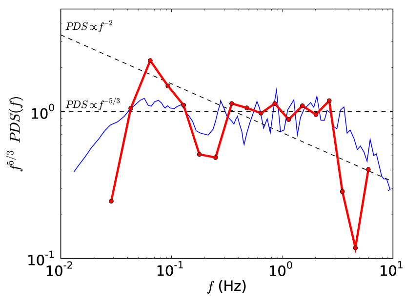
Figure 11: Average power density spectrum of the light-power curves from the extended uniform simulation computed at a distance of $2.5\times 10^{12}$ cm from the center of the star. The thick line shows the power spectrum obtained by averaging 10 light-power curves for viewing angles $\theta_{o}=1$, 2, 3, 4, 5, 6, 7, 8, 9, and $10\arcdeg$ off-axis. The spectrum is multiplied by $f^{5/3}$ to reproduce Figure 2 of Beloborodov et al. (1998), whose data are shown as a thin line. The dashed lines show $PDS(f)\propto{f}^{-5/3}$ and $PDS(f)\propto{f}^{-2}$ spectra for comparison.

The resulting PDS is shown in Figure 11. The spectrum has been multiplied by $f^{5/3}$ to emphasize the slope of the power-law and in an attempt to reproduce, as closely as possible, Fig. 2 of Beloborodov et al. (1998), whose data are shown as a thin line in the figure for comparison. The frequencies of Beloborodov et al. (1998) have been multiplied by a factor 2 to take into account the average redshift of BATSE GRBs. The two spectra show a remarkable qualitative similarity. Both spectra are consistent with a power-law slope $PDS(f)\propto f^{-5/3}$ between a low- and a high-frequency cutoff. The locations of the cutoffs are also compatible with observations for the assumed average redshift of BATSE GRBs.

The rough agreement of the low-frequency cutoff is not surprising since it is due to the overall duration of the burst, which has been set in the simulations to be analogous to the average observed GRB duration. The similarity between the observed and simulated high-frequency cutoffs is more intriguing, although it could be due to either numerical effects or the evolution of the jet. The time scale associated with the $\sim 3$ Hz cutoff in the synthetic spectra is $\delta t\sim 0.33$ s. The jet at the surface of the star has an opening angle of $\sim 4^{\circ}$ (see Figure 6) which corresponds to a transverse size $R_{\perp}=2.8\times 10^{9}$ cm. For a relativistic sound speed $c_{s}=c/\sqrt{3}$, the transverse dimension corresponds to a crossing time of 0.16 s. One possible interpretation is that the cutoff at $\sim 3$ Hz can be identified as the signature of the jet-crossing time of a disturbance that propagates from the side to the axis of the jet, such as a recollimation shock. The difference between the $\sim 6$ Hz cutoff predicted and the $\sim 3$ Hz cutoff seen in our simulations could be because either the “real” opening angle of the jet may be large than the value we use based on our definition in Sect. 3.2, or the characteristic radius at which a shock is crossing the jet may be larger than the original stellar radius. It is also possible that the high-frequency cutoff is a numerical artifact. The cutoff in our data is at $\sim 3$ Hz cutoff, while the maximum frequency we can sample in the extended uniform simulation is $7.5$ Hz, close enough that it is possible the cutoff is a result of resolution effects in the simulation.

The consistency of the observed PDS slope with the synthetic one is, however, more challenging to explain in terms of the physics of the jet-star interaction. It is well known that fully developed turbulence has a 5/3 spectrum (Beloborodov 1998, 2000; Kumar & Narayan 2009; Narayan & Kumar 2009). Turbulent motions are observed in the simulations, but are concentrated in the cocoon material and not in the outflow. Even though the collimation shocks are due to the cocoon pressure on the side of the jet, it is hard to imagine how the turbulence spectrum can be imprinted directly on the jet light-power curves.

The qualitative similarity of the observed PDS with the synthetic one is suggestive that the long time-scale variability in GRBs (down to tenths of seconds) may be due to the jet interaction with the star and not to the inner engine variability. However, GRB light curves show fast spikes with duration of milliseconds or less that cannot be explained as due to the interaction with the stellar progenitor (Walker et al. 2000). It seems therefore that there are two sources of variability in the light curves: the intrinsic variability of the engine, likely operating on the ms time scale since the engine is a compact object, and the star-induced variability, with a cutoff at several tenths of a second, possibly associated with the sound crossing time of the jet at the star’s surface. To study if and how these two variability sources interfere with each other, we compared the PDS of the light-power curve from uniform and variable simulations.

Figure 12 shows the comparison of the PDS from the light-power curves of the various simulations. The power spectrum of the input variability in the variable simulations is also shown. The comparison of the various spectra shows that the two sources of variability have no significant interaction, with the variable spectra being qualitatively similar to the sum of the uniform spectrum - which contains only the star-induced variability - and the input spectrum. The two variable spectra are also qualitatively similar, indicating that the variability of the jet depends only on the variability of the total luminosity of the engine and not on whether the variability is in the entropy or in the baryon loading of the outflow. The PDS of the step simulation also appears similar to the uniform spectrum, with a series of strong resonant peaks at multiples of $5$ Hz, the frequency of the on-off cycle, added at higher frequencies. Again, further simulations will be required to confirm the generality of the conclusions against different progenitors and different jet properties.

4 Discussion and conclusions

We have carried out high-resolution hydrodynamic simulations of the propagation of baryonic GRB jets through their progenitor stars and beyond. For the first time, we explored the consequences of a variable injected luminosity with AMR simulations. Our simulations allowed us to draw a number of conclusions about the role played by the progenitor star material in shaping the final appearance of the prompt light curve:

• The propagation time of the jet in the progenitor star depends on the variability properties of the engine in a complex way. The jet propagation inside the star is affected by the detailed structure of turbulent eddies inside the cocoon, the development of which is highly non-linear and depends on the resolution of the simulation. The propagation time is a very important quantity in any GRB model since it is the quantity that establishes whether the engine is active for a time long enough to power a GRB or not. If the engine is active for a time shorter than the propagation time, it is more likely that an “engine powered” supernova is produced (Soderberg et al. 2010) rather than a successful GRB event. The propagation time also sets the amount of jet energy that is dissipated in the cocoon, available to power a precursor (Ramirez-Ruiz et al. 2002; Lazzati & Begelman 2005) or possibly a short duration GRB (Lazzati et al. 2010). High resolution 3D simulations are required to nail down this important aspect of the jet propagation in the progenitor star.

• Outside their progenitor stars, jets show a much more predictable evolution that does not depend on details. All jets show the three phases of evolution described in MLB07: (i) a wide-angle cocoon phase, (ii) a narrow shocked jet phase lasting 10 to 15 seconds, and (iii) an expanding jet phase. This behavior and its timing seem to be fairly independent of the simulation resolution as well as the details of the central engine.

• Contrary to what was previously thought (Zhang et al. 2003; MLB07), short time-scale variability injected by the central engine is preserved in the jet, even during the shocked phase. The variability injected by the central engine is lost only during a fast initial phase, lasting a few seconds. On the other hand, the interaction of the jet material with the surrounding stellar material creates long time-scale variability even for jets injected with no variability whatsoever. When a variable jet is injected, we find that the progenitor induced variability is not affected, at least at the qualitative level. For the range of simulations studied here, we find that the properties of the variability at time-scales of seconds depend on the progenitor structure and are insensitive to the properties of the outflow injected by the central engine. This is an important finding because it implies that the fast variability in GRB light curves, observable during the bright shocked-jet phase, may depend only on the properties of the GRB engine. We can therefore study the nature of the GRB engine (still clouded in mystery) by studying the properties of the fast variability in GRB light curves.

• Even though we inject an uniform outflow in the center of the star, with no dependence of the jet properties on the polar angle, the jet propagating in the circumstellar material is highly structured. The total observed energy decreases with the off-axis angle as $dE/d\Omega\propto\theta^{-3}$. The peak luminosity, on the other hand, is constant between about $5^{\circ}$ and $20^{\circ}$. This behavior is due to the marked changes in the temporal properties of the jet at different off-axis angles. The diversity of light curves observed in GRB catalogs can therefore be partly attributed to the viewing geometry.

• We computed the power density spectrum (PDS) of light-power curves from an extended simulation (reaching distances from the progenitor star ten times larger than our standard simulations). It shows two important similarities with the PDS of BATSE light curves (Beloborodov et al. 1998; see Fig. 11): a high frequency cutoff at a frequency of few hertz and a power-law behavior consistent with a slope $PDS(f)\propto{}f^{-5/3}$ at lower frequencies. The high frequency cutoff may tentatively be interpreted as the result of the timescale of the propagation of perturbations across the jet, although the cutoff is near the resolution limit of the simulation and may be a numerical artifact. If the presence of the high-frequency cutoff can be confirmed, the coincidence of the simulated cutoff to the observed one may be the first direct confirmation that long duration GRBs are associated with massive stars at all redshifts and not only at $z<1$. The coincidence between the simulated and observed power-law slope suggests instead that the variability that characterizes GRB light curves is mostly due to the interaction of the jet with the progenitor star and not to the GRB engine. Such a result has been obtained under the assumption that the radiation is released at a constant radius and at constant efficiency. In addition, the PDS is steeper, with a slope $PDS(f)\propto{}f^{-2}$ if the initial 5 seconds are removed from the light curve. Since the structure of the head of the jet is affected by the dimensionality of the simulations (cfr. Zhang et al. 2004), we consider this result suggestive and not conclusive.

• A PDS analysis was also performed for the variable simulations (Fig. 12). The low frequency part of the PDS of variable simulations show a power-law behavior qualitatively similar to the one of the uniform simulation. The analogy suggests that, as already discussed in the light curve analysis, the long time-scale variability is a result of the jet-star interaction that does not depend on the details of the engine properties. On the other hand, the high frequency part of the variable PDS has the same qualitative shape of the PDS of the luminosity injected by the engine. This suggests that at high frequencies the propagation of the jet through the star has no impact on the jet structure. The high frequency features are transported unmodified by the relativistic outflow. If our results are confirmed by simulations with different progenitors and jet properties, the analysis of fast variability in GRB light curves could give us important clues to the nature of the GRB engine, while the analysis of the long time-scale variability can yield important clues to the nature of the progenitor star.

There are several potential sources the could create variability in the inner $10^{9}$ cm of the star, including instabilities in the propagating jet, instabilities in the region of jet formation, an inherent variability in the energy available from the central engine (i.e. from a variable accretion rate onto a black hole or a varying spin down rate of a proto-magnetar). Disentangling the sources that give rise to short-timescale variability in observations is likely to be quite challenging. However, whatever variability does arise in the innermost region of the progenitor is preserved during propagation and remains imprinted on the jet that emerges from the stellar surface.

Based on all the evidence gathered in this project, we advance the possibility that variability has two origins, with engine and propagation having comparable roles in shaping the light curve in different regions of the frequency domain. This possibility is shown graphically in Figure 13 that shows the BATSE light curve of GRB 920513 with a thick line underlying the envelope of long time-scale variability due to the jet interaction with the progenitor star. Faster variability is present in the light curve and that is interpreted as variability in the luminosity injected by the central engine at the base of the jet. Observations of high frequency variability, therefore, may offer important clues about the nature and evolution of the central engine.

Figure 1: Luminosity injected by the central engine for the four simulations described in the text. The figure shows only a 3 second zoom of the simulations that last a total time of 50 seconds. The luminosity is normalized to the average isotropic equivalent luminosity of $L_{\{\rm{inj,iso}\}}=3.5\times 10^{52}$ erg/s. The injected luminosity for the variable entropy and variable baryon load simulations is the same.

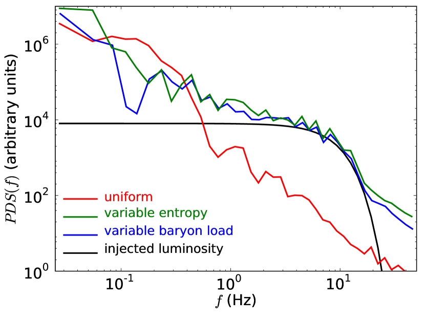
Figure 12: Comparison of the power spectra of variable simulations with the power spectrum from the uniform simulation and the input power spectrum at the base of the jet. Even though the spectra are plotted in arbitrary units, they have not been normalized and can be compared to each other. The power spectra of the variable simulations are similar, showing that the variability properties of the light curve do not depend on the way in which the variability is injected by the GRB engine. The effect of the interaction with the star is clearly present in the PDS curves of the variable simulations as an increase of the power at low frequencies, fully compatible with the low-frequency variability imprinted on the jet from a uniform engine. The two sources of variability add linearly in this case, with the variable simulation spectra well described by the sum of the input variability spectrum and the uniform jet spectrum.

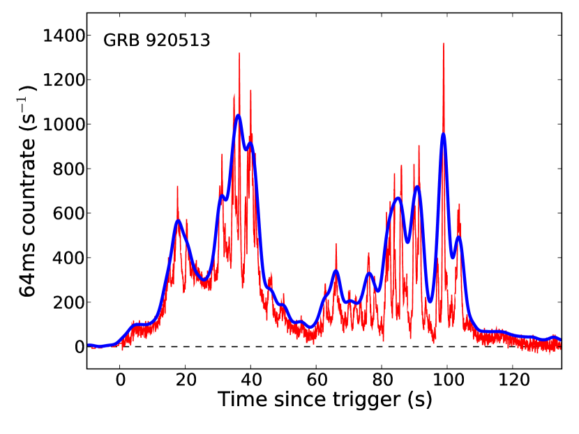
Figure 13: A cartoon showing the realization of the two sources of variability in the light curve of the BATSE GRB 920513. The thin line shows the data from BATSE, displaying the short-timescale variability due to the activity of the central engine. The thick line, on the other hand, emphasizes the long time-scale variability envelope imprinted on the jet by the propagation through the progenitor star.

References

- (1) Abdo, A. A., et al. 2009, Science, 323, 1688
- (2) Aloy, M. A., Müller, E., Ibáñez, J. M., Martí, J. M., & MacFadyen, A. 2000, ApJ, 531, L119
- (3) Aloy, M.-A., Ibáñez, J.-M., Miralles, J.-A., & Urpin, V. 2002, A&A, 396, 693
- (4) Aloy, M. A., & Obergaulinger, M. 2007, Revista Mexicana de Astronomia y Astrofisica, 30, 96
- (5) Beloborodov, A. M., Stern, B. E., & Svensson, R. 1998, ApJ, 508, L25
- (6) Beloborodov, A. M., Stern, B. E., & Svensson, R. 2000, ApJ, 535, 158
- (7) Daigne, F., & Mochkovitch, R. 2002, MNRAS, 336, 1271
- (8) Della Valle, M., et al. 2006, Nature, 444, 1050
- (9) Dermer, C. D., Böttcher, M., & Chiang, J. 1999, ApJ, 515, L49
- (10) Dermer, C. D., Böttcher, M., & Chiang, J. 2000, ApJ, 537, 255
- (11) Fenimore, E. E., Ramirez-Ruiz, E., & Wu, B. 1999, ApJ, 518, L73
- (12) Fryxell, B. et al. 2000 ApJS, 131, 273
- (13) Fynbo, J. P. U., et al. 2006, Nature, 444, 1047
- (14) Gal-Yam, A., et al. 2006, Nature, 444, 1053
- (15) Hjorth, J., et al. 2003, Nature, 423, 847
- (16) Kobayashi, S., Piran, T., & Sari, R. 1997, ApJ, 490, 92
- (17) Kouveliotou, C., Meegan, C. A., Fishman, G. J., Bhat, N. P., Briggs, M. S., Koshut, T. M., Paciesas, W. S., & Pendleton, G. N. 1993, ApJ, 413, L101
- (18) Kumar, P., & Narayan, R. 2009, MNRAS, 395, 472
- (19) Lazzati, D., & Begelman, M. C. 2005, ApJ, 629, 903
- (20) Lazzati, D., Morsony, B. J., & Begelman, M. C. 2009, ApJ, 700, L47 (LMB09)
- (21) Lazzati, D., Morsony, B. J., & Begelman, M. C. 2010, ApJ in press (arXiv:0911.3313v1)
- (22) MacFadyen, A. I., & Woosley, S. E. 1999 ApJ, 524, 262
- (23) MacFadyen, A. I., Woosley, S. E., & Heger, A. 2001 ApJ, 550, 410
- (24) McKinney, J. C., & Narayan, R. 2007, MNRAS, 375, 513
- (25) McKinney, J. C., & Blandford, R. D. 2009, MNRAS, 394, L126
- (26) Mimica, P., Aloy, M. A., Müller, E., & Brinkmann, W. 2005, A&A, 441, 103
- (27) Mimica, P., Aloy, M. A., Müller, E. 2007, A&A, 466, 93
- (28) Mizuta, A., & Aloy, M. A. 2009, ApJ, 699, 1261
- (29) Morsony, B. J., Lazzati, D., & Begelman, M. C. 2007, ApJ, 665, 569 (MLB07)
- (30) Narayan, R., & Kumar, P. 2009, MNRAS, 394, L117
- (31) Ouyed, R., Clarke, D. A., & Pudritz, R. E. 2003, ApJ, 582, 292
- (32) Ramirez-Ruiz, E., MacFadyen, A. I., & Lazzati, D. 2002, MNRAS, 331, 197
- (33) Schaefer, B. E., & Walker, K. C. 1999, ApJ, 511, L89
- (34) Soderberg, A. M., et al. 2009, arXiv:0908.2817
- (35) Stanek, K. Z., et al. 2003, ApJ, 591, L17
- (36) de Ugarte Postigo, A., et al. 2006, ApJ, 648, L83
- (37) Walker, K. C., Schaefer, B. E., & Fenimore, E. E. 2000, ApJ, 537, 264
- (38) Woosley, S. E. 1993, ApJ, 405, 273
- (39) Woosley, S. E., & Bloom, J. S. 2006, ARA&A, 44, 507
- (40) Woosley, S. E., & Heger, A. 2006, ApJ, 637, 914
- (41) Zhang, W., Woosley, S. E., & MacFadyen, A. I. 2003, ApJ, 586, 356
- (42) Zhang, W., Woosley, S. E., & Heger, A. 2004, ApJ, 608, 365