Uniqueness and existence of spirals moving by forced mean curvature motion

Abstract

In this paper, we study the motion of spirals by mean curvature type motion in the (two dimensional) plane. Our motivation comes from dislocation dynamics; in this context, spirals appear when a screw dislocation line reaches the surface of a crystal. The first main result of this paper is a comparison principle for the corresponding parabolic quasi-linear equation. As far as motion of spirals are concerned, the novelty and originality of our setting and results come from the fact that, first, the singularity generated by the attached end point of spirals is taken into account for the first time, and second, spirals are studied in the whole space. Our second main result states that the Cauchy problem is well-posed in the class of sub-linear weak (viscosity) solutions. We also explain how to get the existence of smooth solutions when initial data satisfy an additional compatibility condition.

AMS Classification:

35K55, 35K65, 35A05, 35D40

Keywords:

spirals, motion of interfaces, comparison principle, quasi-linear parabolic equation, viscosity solutions, mean curvature motion.

1 Introduction

In this paper we are interested in curves $(\Gamma_{t})_{t>0}$ in ${\mathbb{R}}^{2}$ which are half lines with an end point attached at the origin. These lines are assumed to move with normal velocity

$$V_{n}=c+\kappa$$ (1.1)

where $\kappa$ is the curvature of the line and $c\in{\mathbb{R}}$ is a given constant. We will see that this problem reduces to the study of the following quasi-linear parabolic equation in non-divergence form

$${r\bar{u}_{t}=c\sqrt{1+r^{2}\bar{u}_{r}^{2}}+\bar{u}_{r}\left(\frac{2+r^{2}\bar{u}_{r}^{2}}{1+r^{2}\bar{u}_{r}^{2}}\right)+\frac{r\bar{u}_{rr}}{1+r^{2}\bar{u}_{r}^{2}}},\qquad t>0,r>0$$ (1.2)

This paper is devoted to the proof of a comparison principle in the class of sub-linear weak (viscosity) solutions and to the study of the associated Cauchy problem.

1.1 Motivations and known results

Continuum mechanics.

From the viewpoint of applications, the question of defining the motion of spirals in a two dimensional space is motivated by the seminal paper of Burton, Cabrera and Frank [2] where the growth of crystals with the vapor is studied. When a screw dislocation line reaches the boundary of the material, atoms are adsorbed on the surface in such a way that a spiral is generated; moreover, under appropriate physical assumptions, these authors prove that the geometric law governing the dynamics of the growth of the spiral is precisely given by (1.1) where $-c$ denotes a critical value of the curvature. We mention that there is an extensive literature in physics dealing with crystal growth in spiral patterns.

Different mathematical approaches.

First and foremost, defining geometric flows by studying non-linear parabolic equations is an important topic both in analysis and geometry. Giving references in such a general framework is out of the scope of this paper. As far as the motion of spirals is concerned, the study of the dynamics of spirals have been attracting a lot of attention for more than ten years. Different methods have been proposed and developed in order to define solutions of the geometric law (1.1). A brief list is given here. A phase-field approach was first proposed in [14] and the reader is also referred to [16, 17]. Other approaches have been used; for instance, “self-similar” spirals are constructed in [13] by studying an ordinary differential equation. In [10], spirals moving in (compact) annuli with homogeneous Neumann boundary condition are constructed. From a technical point of view, the classical parabolic theory is used to construct smooth solutions of the associated partial differential equation; in particular, gradient estimates are derived. We point out that in [10], the geometric law is anisotropic, and is thus more general than (1.1). In [22, 18], the geometric flow is studied by using the level-set approach [19, 3, 7]. As in [10], the author of [18] considers spirals that typically move into a (compact) annulus and reaches the boundary perpendicularly.

The starting point of this paper is the following fact: to the best of our knowledge, no geometric flows were constructed to describe the dynamics of spirals by mean curvature by taking into account both the singularity of the pinned point and the unboundedness of the domain.

The equation of interest.

We would like next to explain with more details the main aims of our study. By parametrizing spirals, we will see (cf. Subsection 1.2) that the geometric law (1.1) is translated into the quasi-linear parabolic equation (1.2). We note that the coefficients are unbounded (they explode linearly with respect to $r$) and that the equation is singular: indeed, as $r\to 0$, either $ru_{t}\to 0$ or first order terms explode. Moreover, initial data are also unbounded. In such a framework, we would like to achieve: uniqueness of weak (viscosity) solutions for the Cauchy problem for a large class of initial data, to construct a unique steady state (i.e. a solution of the form $\lambda t+\bar{\varphi}(r)$), and finally to show the convergence of general solutions of the Cauchy problem to the steady state as time goes to infinity. This paper is mainly concerned with proving a uniqueness result and constructing a weak (viscosity) solution; the study of large time asymptotic will be achieved in [9].

Classical parabolic theory.

Classical parabolic theory [8, 15] could help us to construct solutions but there are major difficulties to overcome. For instance, Giga, Ishimura and Kohsaka [10] studied a generalization of (1.2) in domains of the form $R_{a,b}={\color[rgb]{0,0,0}\{a<r<b\}}$ with $a>0$ and $b>0$, with Neumann boundary conditions at $r=a,b$. Roughly speaking, we can say that our goal is to see what happens when $a\to 0$ and $b\to\infty$. First, we mentioned above that the equation is not (uniformly) parabolic in the whole domain $R_{0,\infty}={\color[rgb]{0,0,0}\left\{0<r<+\infty\right\}}$. Second, in such analysis, the key step is to obtain gradient estimates. Unfortunately, the estimates from [10] in the case of (1.2) explode as $a$ goes to $0$. Third, once a solution is constructed, it is natural to study uniqueness but even in the setting of classical solutions there are substantial difficulties. To conclude, classical parabolic theory can be useful in order to get existence results, keeping in mind that getting gradient estimates for (1.2) is not at all easy, but such techniques will not help in proving uniqueness.

Recently, several authors studied uniqueness of quasilinear equations with unbounded coefficients (see for instance [1, 4]) by using viscosity solution techniques for instance. But unfortunately, Eq. (1.2) does not satisfy the assumptions of these papers.

Main new ideas.

New ideas are thus necessary to handle these difficulties, both for existence and uniqueness. As far as uniqueness is concerned, one has to figure out what is the relevant boundary condition at $r=0$. We remark that solutions of (1.2) satisfy at least formally a Neumann boundary condition at the origin

$$0=c+2\bar{u}_{r}\quad\mbox{for}\quad r=0.$$ (1.3)

In some sense, we thus can say that the boundary condition is embedded into the equation. Second, taking advantage of the fact that the Neumann condition is compatible with the comparison principle, viscosity solution techniques (also used in [1]) permit us to get uniqueness even if the equation is degenerate and also in a very large class of weak (sub- and super-) solutions.

But there are remaining difficulties to be overcome. First, the Boundary Condition (1.3) is only true asymptotically (as $r\to 0$) and the fact that it is embedded into the equation makes it difficult to use. We will overcome this difficulty by making a proper change of variables (namely $x=\ln r$, see below for further details) and proving a comparison principle (whose proof is rather involved; in particular many new arguments are needed in compare with the classical case) in this framework. Second, classical viscosity solution techniques for parabolic equations do not apply directly to (1.2) because of polar coordinates. More precisely, the equation do not satisfy the fundamental structure conditions as presented in [5, Eq. (3.14)] when polar coordinates are used. But the mean curvature equation has been extensively studied in Cartesian coordinates [7, 3]. Hence this set of coordinates should be used, at least far from the origin.

Perron’s method and smooth solutions.

We hope we convinced the reader that it is really useful, if not mandatory, to use viscosity solution techniques to prove uniqueness. It turns out that it can also be used to construct solutions by using Perron’s method [12]. This technique requires to construct appropriate barriers and we do so for a large class of initial data. The next step is to prove that these weak solutions are smooth if additional growth assumptions on derivatives of initial data are imposed; we get such a result by deriving non-standard gradient estimates (with viscosity solution techniques too).

We would like also to shed some light on the fact that this notion of solution is also very useful when studying large time asymptotic (and more generally to pass to the limit in such non-linear equations). Indeed, convergence can be proved by using the half-relaxed limit techniques if one can prove a comparison principle. See [9] for more details.

1.2 The geometric formulation

In this section, we make precise the way spirals are defined. We will first define them as parametrized curves.

Parametrization of spirals.

We look for interfaces $\Gamma$ parametrized as follows: $\Gamma=\{re^{-i\bar{u}(r)}:r\geq 0\}{\color[rgb]{0,0,0}\ \subset{\mathbb{C}}}$ for some function $\bar{u}:[0,+\infty)\to{\mathbb{R}}$. If now the spiral moves, i.e. evolves with a time variable $t>0$, then the function $\bar{u}$ also depends on $t>0$.

Definition 1.1 (Spirals).

A moving spiral is a family of curves $(\Gamma_{t})_{t>0}$ of the following form

$$\Gamma_{t}=\{re^{i\theta}:r>0,\theta\in{\mathbb{R}},\;\theta+\bar{u}(t,r)=0\}$$ (1.4)

for some function $\bar{u}:[0,+\infty)\times[0,+\infty)\to{\mathbb{R}}$. This curve is oriented by choosing the normal vector field equal to $(-i+r\partial_{r}\bar{u}(t,r))e^{-i\bar{u}(t,r)}$.

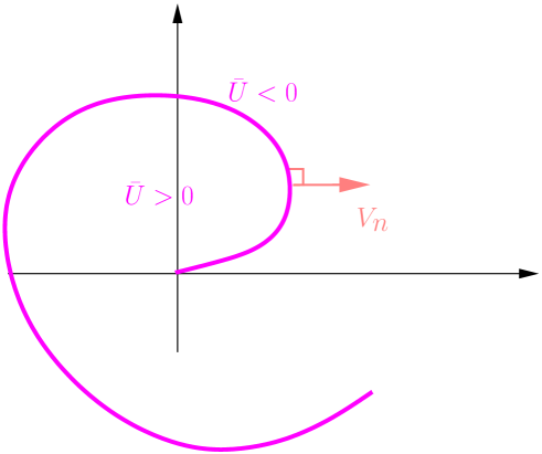
Figure 1: Motion of the spiral

With the previous definition in hand, the geometric law (1.1) implies that $\bar{u}$ satisfies (1.2) with the initial condition

$$\bar{u}(0,r)=\bar{u}_{0}(r)\quad\mbox{for}\quad r\in(0,+\infty)\,.$$ (1.5)

Link with the level-set approach.

In view of (1.4), we see that our approach is closely related to the level-set one. We recall that the level-set approach was introduced in [19, 7, 3]; in particular, it permits to construct an interface moving by mean curvature type motion, that is to say satisfying the geometric law (1.1). It consists in defining the interface $\Gamma_{t}$ as the $0$-level set of a function $\tilde{U}(t,\cdot)$ and in remarking that the geometric law is verified only if $\tilde{U}$ satisfies a non-linear evolution equation of parabolic type. In an informal way, we can say that the quasi-linear evolution equation (1.2) is a ”graph” equation associated with the classical mean curvature equation (MCE), but written in polar coordinates.

More precisely, if ${\color[rgb]{0,0,0}\tilde{U}(t,X)=\theta+\bar{u}(t,r)}$ with $X{\color[rgb]{0,0,0}=(r\cos\theta,r\sin\theta)}\in{\mathbb{R}}^{2}$, then $\bar{u}$ will satisfy (1.2) as long as $\tilde{U}$ solves the following level-set equation

$$\tilde{U}_{t}=c|D_{X}\tilde{U}|+\widehat{D_{X}\tilde{U}}^{\perp}\cdot D^{2}_{XX}\tilde{U}\;\widehat{D_{X}\tilde{U}}^{\perp}{\color[rgb]{0,0,0}\quad\mbox{for}\quad X\not=0}$$ (1.6)

(where $\hat{p}=p/|p|$ and $p^{\perp}=(-p_{2},p_{1})$ for $p=(p_{1},p_{2})\in{\mathbb{R}}^{2}$). Notice that the angle $\theta$ is multivalued, i.e. only defined modulo $2\pi$. Such an approach is for instance systematically developed in [18].

1.3 Main results

Comparison principle.

Our first main result is a comparison principle: it says that all sub-solutions lie below all super-solutions, provided they are ordered at initial time.

Theorem 1.2 (Comparison principle for (1.2)).

Assume that $\bar{u}_{0}:(0,+\infty)\to{\mathbb{R}}$ is a globally Lipschitz continuous function. Consider a sub-solution $\bar{u}$ and a super-solution $\bar{v}$ of (1.2),(1.5) (in the sense of Definition 2.1) such that there exist $C_{1}>0$ and for all $t\in[0,T)$ and $r>0$,

$$\bar{u}(t,r)-\bar{u}_{0}(r)\leq C_{1}\quad\text{and}\quad\bar{v}(t,r)-\bar{u}_{0}(r)\geq-C_{1}.$$ (1.7)

If $\bar{u}(0,r)\leq\bar{u}_{0}(r)\leq\bar{v}(0,r)$ for all $r\geq 0$, then $\bar{u}\leq\bar{v}$ in $[0,T)\times(0,+\infty)$.

Remark 1.3.

The growth of the sub-solution $u$ and the super-solution $v$ is made precise by assuming Condition (1.7). Such a condition is motivated by the large time asymptotic study carried out in [9]; indeed, we construct in [9] a global solution of the form $\lambda t+\bar{u}_{0}(r)$.

The proof of Theorem 1.2 is rather involved and we will first state and prove a comparison principle in the set of bounded functions for a larger class of equations (see Theorem 3.1). We do so in order to exhibit the structure of the equation that makes the proof work. We then turn to the proof of Theorem 1.2.

Both proofs are based on the doubling of variable method, which consists in regularizing the sub- and super-solutions. Obviously, this is a difficulty here because one end point of the curve is attached at the origin and the doubling of variables at the origin is not well defined. To overcome this difficulty, we work with logarithmic coordinates $x=\ln r$ for $r$ close to $0$. But then the equation becomes

$$u_{t}=ce^{-x}\sqrt{1+u_{x}^{2}}+e^{-2x}u_{x}+e^{-2x}\frac{u_{xx}}{1+u_{x}^{2}}$$

We then apply the doubling of variables in the $x$ coordinates. There is a persistence of the difficulty, because we have now to bound terms like

$$A:=ce^{-x}\sqrt{1+u_{x}^{2}}-ce^{-y}\sqrt{1+v_{y}^{2}}$$

that can blow up as $x,y\to-\infty$. We are lucky enough to be able to show roughly speaking that $A$ can be controlled by the doubling of variable of the term $e^{-2x}u_{x}$ which appears to be the main term (in a certain sense) as $x$ goes to $-\infty$.

In view of the study from [9], $\bar{u}_{0}$ has to be chosen sub-linear in Cartesian coordinates and thus so are the sub- and super-solutions to be compared. The second difficulty arises when passing to logarithmic coordinates for large $r$’s; indeed, the sub-solution and the super-solution then grow exponentially in $x=\ln r$ at infinity and we did not manage to adapt the previous reasoning in this setting. There is for instance a similar difficulty when dealing with the mean curvature equatio. Indeed, in this framework, for super-linear initial data, the uniqueness of the solution is not known in full generality (see [1, 4]). In other words, the change of variables do not seem to work far from the origin. We thus have to stick to Cartesian coordinates for large $r$’s (using a level-set formulation) and see the equation in different coordinates when $r$ is either small or large (see Section 4).

Existence theorem.

In order to get an existence theorem, we have to restrict the growth of derivatives of the initial condition. We make the following assumptions: the initial condition is globally Lipschitz continuous and its mean curvature is bounded. We recall that the mean curvature of a spiral parametrized by $\bar{u}$ is defined by

$$\kappa_{\bar{u}}(r)=u_{r}\left(\frac{2+(r\bar{u}_{r})^{2}}{(1+(r\bar{u}_{r})^{2})^{\frac{3}{2}}}\right)+\frac{r\bar{u}_{rr}}{(1+(r\bar{u}_{r})^{2})^{\frac{3}{2}}}.$$

We can now state our second main result.

Theorem 1.4 (The general Cauchy problem).

Consider $\bar{u}_{0}\in{\color[rgb]{0,0,0}W^{2,\infty}_{loc}(0,+\infty)}$. Assume that $\bar{u}_{0}$ is globally Lipschitz continuous and that $\kappa_{\bar{u}_{0}}\in L^{\infty}(0,+\infty)$. Then there exists a unique solution $u$ of (1.2),(1.5) on $[0,+\infty)\times(0,+\infty)$ (in the sense of Definition 2.1) such that for all $T>0$, there exists $\bar{C}_{T}>0$ such that for all $t\in{\color[rgb]{0,0,0}[0,T)}$ and $r>0$,

$$|\bar{u}(t,r)-\bar{u}_{0}(r)|\leq{\color[rgb]{0,0,0}\bar{C}_{T}}.$$ (1.8)

Moreover, $\bar{u}$ is Lipschitz continuous with respect to space and $\frac{1}{2}$-Hölder continuous with respect to time. More precisely, there exists a constant $C$ depending only on $|(\bar{u}_{0})_{r}|_{\infty}$ and $|\kappa_{\bar{u}_{0}}|_{\infty}$ such that

$$|\bar{u}(t,r+\rho)-\bar{u}(t,r)|\leq C|\rho|$$

and

$$|\bar{u}(t+h,r)-\bar{u}(t,r)|\leq C\sqrt{|h|}.$$ (1.9)

Remark 1.5.

Notice that Theorem 1.4 allows us to consider an initial data $\bar{u}_{0}$ which does not satisfy the compatibility condition (1.3), like for instance $\bar{u}_{0}\equiv 0$ with $c=1$. Notice also that we do not know if the solution constructed in Theorem 1.4 is smooth (i.e. belongs to $C^{\infty}((0,+\infty)^{2})$).

To get such a result, we first construct smooth solutions requiring that the compatibility condition (1.3) is satisfied by the initial datum, like in the following result.

Theorem 1.6 (Existence and uniqueness of smooth solutions for the Cauchy problem).

Assume that $\bar{u}_{0}\in W^{2,\infty}_{loc}(0,+\infty)$ with

$$(\bar{u}_{0})_{r}\in W^{1,\infty}(0,+\infty)\quad\mbox{or}\quad\kappa_{\bar{u}_{0}}\in L^{\infty}(0,+\infty)$$

and that it satisfies the following compatibility condition for some $r_{0}>0$:

$$|c+\kappa_{\bar{u}_{0}}|\leq Cr\quad{\rm for}\quad 0\leq r\leq{\color[rgb]{0,0,0}r_{0}}.$$ (1.10)

Then there exists a unique continuous function: $\bar{u}:[0,+\infty)\times[0,+\infty)$ which is $C^{\infty}$ in $(0,+\infty)\times(0,+\infty)$, which satisfies (1.2),(1.5) (in the sense of Definition 2.1), and such that there exists $\bar{C}>0$ such that

$$|\bar{u}(t,r+\rho)-\bar{u}(t,r)|\leq\bar{C}|\rho|$$

and

$$|\bar{u}(t+h,r)-\bar{u}(t,r)|\leq\bar{C}|h|.$$ (1.11)

Remark 1.7.

Condition (1.10) allows us also to improve the Hölder estimate (1.9) and to replace it by the Lipschitz estimate (1.11). With the help of this Lipschitz estimate (1.11), we can conclude that the solution constructed in Theorem 1.6 is smooth. Notice also that our space-time Lipschitz estimates on the solution allow us to conclude that $\bar{u}(t,\cdot)$ satisfies (1.10) with the constant $C$ replaced by some possible higher constant. This implies in particular that $\bar{u}(t,\cdot)$ satisfies the compatibility condition (1.3) for all time $t\geq 0$.

Open questions.

A. Weaker conditions on the initial data
It would be interesting to investigate the existence/non-existence and uniqueness/non-uniqueness of solutions when we allow the initial data $\bar{u}_{0}$ to be less than globally Lipschitz. For instance what happens when the initial data describes an infinite spiral close to the origin $r=0$, with either $\bar{u}_{0}(0^{+})=+\infty$ or $\bar{u}_{0}(0^{+})=-\infty$? On the other hand, what happens if the growth of $\bar{u}_{0}$ is super-linear as $r$ goes to $+\infty$?
B. More general shapes than spiral
One of our main limitation to study only the evolution of spirals in this paper is that we were not able to prove a comparison principle in the case of the general level-set equation (1.6). The difficulty is the fact that the gradient of the level-set function $\tilde{U}$ may degenerate exactly at the origin where the curve is attached. The fact that a spiral-like solution is a graph $\theta=-\bar{u}(t,r)$ prevents the vanishing of the gradient of $\tilde{U}$ at the origin $r=0$. If now we consider more general curves attached at the origin, it would be interesting to study the existence and uniqueness/non-uniqueness of solutions with general initial data, like the curves on Figure 2.

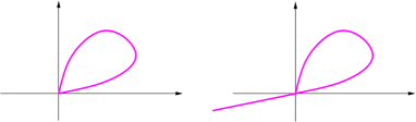
Figure 2: Examples of non spiral initial data

Organization of the article.

In Section 2, we recall the definition of viscosity solutions for the quasi-linear evolution equation of interest in this paper. The change of variables that will be used in the proof of the comparison principle is also introduced. In Section 3, we give the proof of Theorem 1.2 in the case of bounded solutions. The proof in the general case is given in Section 4. In Section 5, a classical solution is constructed under an additional compatibility condition on the initial datum (see Theorem 1.6). First, we construct a viscosity solution by Perron’s method (Subsection 5.1); second, we derive gradient estimates (Subsection 5.2); third, we explain how to prove that the viscosity solution is in fact a classical one (Subsection 5.3). The construction of the solution without compatibility assumption (Theorem 1.4) is made in Section 6. Finally, proofs of technical lemmas are gathered in Appendix A.

Notation.

If $a$ is a real number, $a_{+}$ denotes $\max(0,a)$ and $a_{-}$ denotes $\max(0,-a)$ If $p=(p_{1},p_{2})\in{\mathbb{R}}^{2}$, $p\neq 0$, then $\hat{p}$ denotes $p/|p|$ and $p^{\perp}$ denotes $(-p_{2},p_{1})$.

2 Preliminaries

2.1 Viscosity solutions for the main equation

In view of (1.2), it is convenient to introduce the following notation

$$\bar{F}(r,q,Y)=c\sqrt{1+r^{2}q^{2}}+q\left(\frac{2+r^{2}q^{2}}{1+r^{2}q^{2}}\right)+\frac{rY}{1+r^{2}q^{2}}.$$ (2.12)

We first recall the notion of viscosity solution for an equation such as (1.2).

Definition 2.1 (Viscosity solutions for (1.2),(1.5)).

Let $T\in(0,+\infty]$. A lower semi-continuous (resp. upper semi-continuous) function $u:[0,T)\times(0,+\infty)\to{\mathbb{R}}$ is a (viscosity) super-solution (resp. sub-solution) of (1.2),(1.5) on $[0,T)\times(0,+\infty)$ if for any $C^{2}$ test function $\phi$ such that $u-\phi$ reaches a local minimum (resp. maximum) at $(t,r)\in[0,T)\times(0,+\infty)$, we have

• If $t>0$:

  $$r\phi_{t}\geq\bar{F}(r,\phi_{r},\phi_{rr})\quad\bigg{(}\text{resp. }r\phi_{t}\leq\bar{F}(r,\phi_{r},\phi_{rr})\bigg{)}.$$

• If $t=0$:

  $$u(0,r)\geq\bar{u}_{0}(r)\quad\bigg{(}{\rm resp.}\;u(0,r)\leq\bar{u}_{0}(r)\bigg{)}.$$

A continuous function $u:[0,T)\times(0,+\infty)\to{\mathbb{R}}$ is a (viscosity) solution of (1.2),(1.5) on $[0,T)\times(0,+\infty)$ if it is both a super-solution and a sub-solution.

Remark 2.2.

We do not impose any condition at $r=0$; in other words, it is not necessary to impose a condition on the whole parabolic boundary of the domain. This is due to the “singularity” of our equation at $r=0$.

Since we only deal with this weak notion of solution, (sub-/super-)solutions will always refer to (sub-/super-)solutions in the viscosity sense.

When constructing solutions by Perron’s method, it is necessary to use the following classical discontinuous stability result. The reader is referred to [3] for a proof.

Proposition 2.3 (Discontinuous stability).

Consider a family $(u_{\alpha})_{\alpha\in\mathcal{A}}$ of sub-solutions of (1.2),(1.5) which is uniformly bounded from above. Then the upper semi-continuous envelope of $\sup_{\alpha\in\mathcal{A}}u_{\alpha}$ is a sub-solution of (1.2),(1.5).

2.2 A change of unknown function

We will make use of the following change of unknown function: $u(t,x)=\bar{u}(t,r)$ with $x=\ln r$ satisfies for all $t>0$ and $x\in{\mathbb{R}}$

$$u_{t}=ce^{-x}\sqrt{1+u_{x}^{2}}+e^{-2x}u_{x}+e^{-2x}\frac{u_{xx}}{1+u_{x}^{2}}$$ (2.13)

submitted to the initial condition: for all $x\in{\mathbb{R}}$,

$$u(0,x)=u_{0}(x)$$ (2.14)

where $u_{0}(x)=\bar{u}_{0}(e^{x})$. Eq. (2.13) can be rewritten $u_{t}=F(x,u_{x},u_{xx})$ with

$$F(x,p,X)=ce^{-x}\sqrt{1+p^{2}}+e^{-2x}p+e^{-2x}\frac{X}{1+p^{2}}.$$ (2.15)

Remark that functions $F$ and $\bar{F}$ are related by the following formula

$$F(x,u_{x},u_{xx})=\frac{1}{r}\bar{F}(r,\bar{u}_{r},\bar{u}_{rr})\,.$$ (2.16)

Since the function $\ln$ is increasing and maps $(0,+\infty)$ onto ${\mathbb{R}}$, we have the following elementary lemma which will be used repeatedly throughout the paper.

Lemma 2.4 (Change of variables).

A function $\bar{u}$ is a solution of (1.2),(1.5) if and only if the corresponding function $u$ is a solution of (2.13)-(2.14) with $u_{0}(x)=\bar{u}_{0}(e^{x})$.

The reader is referred to [5] (for instance) for a proof of such a result. When proving the comparison principle in the general case, we will also have to use Cartesian coordinates. From a technical point of view, the following lemma is needed.

Lemma 2.5 (Coming back to the Cartesian coordinates).

We consider a sub-solution $u$ (resp. super-solution $v$) of (2.13)-(2.14) and we define the function $\tilde{U}$ (resp. $\tilde{V}$) $:(0,+\infty)\times{\mathbb{R}}^{2}\to{\mathbb{R}}$ by

$$\tilde{U}(t,X)=\theta(X)+u(t,x(X))\quad\text{\rm(resp. }\quad\tilde{V}(t,Y)=\theta(Y)+u(t,x(Y))\text{)}$$

where $(\theta(Z),x(Z))$ is defined such that $Z=e^{x(Z)+i\theta(Z)}\neq 0$. Then $\tilde{U}$ (resp. $\tilde{V}$) is sub-solution (resp. super-solution) of

$$\left\{\begin{array}[]{l}\displaystyle{w_{t}=c|Dw|+\frac{Dw^{\perp}}{|Dw|}D^{2}w\frac{Dw^{\perp}}{|Dw|}}\\ \\ w(0,x)=\theta(X)+\bar{u}_{0}(x(X)).\end{array}\right.$$ (2.17)

Remark 2.6.

In Lemma 2.5, for $Z\not=0$, the angle $\theta(Z)$ is only defined modulo $2\pi$, but is locally uniquely defined by continuity. Then $D\theta,D^{2}\theta$ are always uniquely defined.

3 A comparison principle for bounded solutions

As explained in the introduction, we first prove a comparison principle for (1.2) in the class of bounded weak (viscosity) solutions. In comparison with classical comparison results for geometric equations (see for instance [7, 3, 20, 11]), the difficulty is to handle the singularity at the origin ($r=0$).

In order to clarify why a comparison principle holds true for such a singular equation, we consider the following generalized case

$$\bar{u}_{t}=\frac{\bar{b}(\bar{u}_{r},r\bar{u}_{r})}{r}+\sigma^{2}(r\bar{u}_{r})\bar{u}_{rr}$$ (3.18)

which can be written, with $x=\ln r$,

$$u_{t}=e^{-x}b(e^{-x}u_{x},u_{x})+e^{-2x}\sigma^{2}(u_{x})u_{xx}$$ (3.19)

where $b(q,p)=\bar{b}(q,p)-\sigma^{2}(p)q$.

Assumption on $\mathbf{(}b,\sigma)$.

• $\sigma\in W^{1,\infty}({\mathbb{R}})$;

• There exists $\delta_{1},\delta_{2},\delta_{3},\delta_{4}>0$ such that

  • for all $q\in{\mathbb{R}}$ and $p_{1},p_{2}\in{\mathbb{R}}$,

    $$|b(q,p_{1})-b(q,p_{2})|\leq\delta_{1}|p_{1}-p_{2}|;$$

  • for all $p\in{\mathbb{R}}$ and $q_{1}\leq q_{2}$,

    $$\delta_{2}(q_{2}-q_{1})\leq b(q_{2},p)-b(q_{1},p);$$

    $$|b(q_{1},p)-b(q_{2},p)|\leq\delta_{3}|q_{1}-q_{2}|;$$

  • for all $p\in{\mathbb{R}}$

    $$|b(0,p)|\leq\delta_{4}\sqrt{1+|p|^{2}}$$

  • we have $\|\sigma\|_{\infty}^{2}<2\delta_{2}$.

In our special case, $\sigma(p)=(1+p^{2})^{-\frac{1}{2}}$ and $b(q,p)=c\sqrt{1+p^{2}}+q$, and the assumption on $(b,\sigma)$ is satisfied.

Theorem 3.1 (Comparison principle for (3.18)-(2.14)).

Assume that $u_{0}:(0,+\infty)\to{\mathbb{R}}$ is Lipschitz continuous. Consider a bounded sub-solution $u$ and a bounded super-solution $v$ of (3.18),(2.14) in the sense of Definition 2.1 with $\bar{F}$ given by the right hand side of (3.18). Then $u\leq v$ in $(0,+\infty)\times{\mathbb{R}}$.

Remark 3.2.

For radial solutions of the heat equation $u_{t}=\Delta u$ on ${\mathbb{R}}^{n}\backslash\left\{0\right\}$, we get $b(q,p)=(n-1)q$ and $\sigma(p)=1$. Therefore the assumption on $(b,\sigma)$ is satisfied if and only if $1<2(n-2)$. Notice that in particular for $n=2$ this assumption is not satisfied.

Proof of Theorem 3.1.

We classically fix $T>0$ and argue by contradiction by assuming that

$$M=\sup_{0<t<T,x\in{\mathbb{R}}}(u(t,x)-v(t,x))>0.$$

Lemma 3.3 (Penalization).

For $\alpha,\varepsilon,\eta>0$ small enough, and any $K\geq 0$, the supremum

$$M_{\varepsilon,\alpha}=\sup_{0<t<T,x,y\in{\mathbb{R}}}\left\{u(t,x)-v(t,y)-e^{Kt}\frac{(x-y)^{2}}{2\varepsilon}-\frac{\eta}{T-t}-\alpha\frac{x^{2}}{2}\right\}$$

is attained at $(t,x,y)$ with $t>0$, $M_{\varepsilon,\alpha}>M/3>0$, $|x-y|\leq C_{0}\sqrt{\varepsilon}$ and $\alpha|x|\leq C_{0}\sqrt{\alpha}$ for some $C_{0}>0$ only depending on $\|u\|_{\infty}$ and $\|v\|_{\infty}$.

Proof of Lemma 3.3.

The fact that $M>0$ means that there exist $t^{*}>0$ and $x^{*}\in{\mathbb{R}}$ such that

$$u(t^{*},x^{*})-v(t^{*},x^{*})\geq M/2>0.$$

Since $u$ and $v$ are bounded functions, $M_{\varepsilon,\alpha}$ is attained at a point $(t,x,y)$. By optimality of $(t,x,y)$, we have in particular

$$u(t,x)-v(t,y)-e^{Kt}\frac{(x-y)^{2}}{2\varepsilon}-\frac{\eta}{T-t}-\alpha\frac{x^{2}}{2}\\ \geq u(t^{*},x^{*})-v(t^{*},x^{*})-\frac{\eta}{T-t^{*}}-\alpha\frac{(x^{*})^{2}}{2}\geq M/3$$

for $\alpha$ and $\eta$ small enough (only depending on $M$). In particular,

$$\frac{(x-y)^{2}}{2\varepsilon}+\alpha\frac{x^{2}}{2}\leq\|u\|_{\infty}+\|v\|_{\infty}\,.$$

Hence, there exists a constant $C_{0}$ only depending on $\|u\|_{\infty}$ and $\|v\|_{\infty}$ such that

$$|x-y|\leq C_{0}\sqrt{\varepsilon}\quad\text{ and }\quad\alpha|x|\leq C_{0}\sqrt{\alpha}\,.$$ (3.20)

Assume that $t=0$. In this case, we use the fact that $u_{0}$ is Lipschitz continuous and (3.20) in order to get

$$\frac{M}{3} \leq u_{0}(x)-u_{0}(y)\leq\|Du_{0}\|_{\infty}|x-y|\leq C_{0}\|Du_{0}\|_{\infty}\sqrt{\varepsilon}$$

which is absurd for $\varepsilon$ small enough (depending only on $M,C_{0}$ and $\|Du_{0}\|_{\infty}$). Hence $t>0$ and the proof of the lemma is complete. ∎

In the remaining of the proof, $\varepsilon$ is fixed (even if we will choose it small enough) and $\alpha$ goes to $0$ (even if it is not necessary to pass to the limit). In view of the previous discussion, we can assume that, for $\varepsilon$ small enough, we have $t>0$ for all $\alpha>0$ small enough (independent on $\varepsilon$). We thus can write two viscosity inequalities. It is then classical to use Jensen-Ishii’s Lemma and combine viscosity inequalities in order to get the following result.

Lemma 3.4 (Consequence of viscosity inequalities).

$$\frac{\eta}{(T-t)^{2}}+Ke^{Kt}\frac{(x-y)^{2}}{2\varepsilon}\leq e^{-x}b(e^{-x}(p+\alpha x),p+\alpha x)-e^{-y}b(e^{-y}p,p)\\ +e^{-2x}\|\sigma\|_{\infty}^{2}\alpha+\frac{e^{Kt}}{\varepsilon}(e^{-x}\sigma(p+\alpha x)-e^{-y}\sigma(p))^{2}$$ (3.21)

where $p=e^{Kt}\frac{(x-y)}{\varepsilon}$.

Proof of Lemma 3.4.

Jensen-Ishii ’s Lemma [5] implies that for all $\gamma_{1}>0$, there exist four real numbers $a,b,A,B$ such that

$$a \leq e^{-x}b(e^{-x}(p+\alpha x),p+\alpha x)+e^{-2x}\sigma^{2}(p+\alpha x)(A+\alpha)$$ (3.22)

$$b \geq e^{-y}b(e^{-y}p,p)+e^{-2y}\sigma^{2}(p)B$$ (3.23)

Moreover $a,b$ satisfy the following inequality

$$a-b\geq\frac{\eta}{(T-t)^{2}}+Ke^{Kt}\frac{(x-y)^{2}}{2\varepsilon}$$ (3.24)

(it is in fact an equality) and for any $\gamma_{1}>0$ small enough, there exist two real numbers $A,B$ satisfying the following matrix inequality

$$\left[\begin{array}[]{cc}A&0\\ 0&-B\end{array}\right]\leq\frac{e^{Kt}}{\varepsilon}(1+{\gamma_{1}})\left[\begin{array}[]{cc}1&-1\\ -1&1\end{array}\right]\,.$$

This matrix inequality implies

$$A\xi_{1}^{2}\leq B\xi_{2}^{2}+\frac{e^{Kt}}{\varepsilon}(1+{\gamma_{1}})(\xi_{1}-\xi_{2})^{2}$$ (3.25)

for all $\xi_{1},\xi_{2}\in{\mathbb{R}}$. Use this inequality with $\xi_{1}=e^{-x}\sigma(p+\alpha x)$ and $\xi_{2}=e^{-y}\sigma(p)$ and let $\gamma_{1}\to 0$ in order to get the desired inequality. ∎

We can next make appear which error terms depend on $\alpha$ and which ones depend on $\varepsilon$. For all $\gamma_{2}>0$,

$$\frac{\eta}{T^{2}}+Ke^{Kt}\frac{(x-y)^{2}}{2\varepsilon}\leq T_{\alpha}+T_{\varepsilon}$$ (3.26)

where

$$T_{\alpha}=e^{-x}b(e^{-x}(p+\alpha x),p+\alpha x)-e^{-x}b(e^{-x}p,p)\\ +\|\sigma\|_{\infty}^{2}e^{-2x}\alpha+(1+\gamma_{2}^{-1})\frac{e^{Kt-2x}}{\varepsilon}\|\sigma^{\prime}\|_{\infty}^{2}(\alpha x)^{2}$$

and $T_{\varepsilon}=T_{\varepsilon}^{1}+T_{\varepsilon}^{2}$ with

$$T_{\varepsilon}^{1}=e^{-x}b(e^{-x}p,p)-e^{-y}b(e^{-y}p,p)\quad\text{and}\quad T_{\varepsilon}^{2}=(1+\gamma_{2})\|\sigma\|^{2}_{\infty}\frac{e^{Kt-2x}}{\varepsilon}(1-e^{x-y})^{2}.$$

It remains to estimate $T_{\varepsilon}$.

Lemma 3.5 (Estimate for $T_{\varepsilon}$).

For all $\gamma_{3}>0$,

$$T_{\varepsilon}\leq((C-2\delta_{2})e^{-2x}+\gamma_{3})e^{Kt}\frac{(x-y)^{2}}{\varepsilon}+\gamma_{3}\varepsilon$$ (3.27)

where $C=\frac{\delta_{4}^{2}}{4\gamma_{3}}+(1+\gamma_{2})\|\sigma\|^{2}_{\infty}+o_{\varepsilon}(1)$.

Proof.

Through a Taylor expansion, we obtain

$$T_{\varepsilon}^{1}= -e^{-y_{\theta}}b(e^{-y_{\theta}}p,p)(x-y)-e^{-2y_{\theta}}\partial_{q}b(e^{-y_{\theta}}p,p)p(x-y)$$

$$\leq -\varepsilon e^{-Kt}b(e^{-y_{\theta}}p,p)e^{-y_{\theta}}p-\delta_{2}e^{Kt-2y_{\theta}}\frac{(x-y)^{2}}{\varepsilon}$$

where $y_{\theta}=\theta y+(1-\theta)x$ for some $\theta\in[0,1]$, and we have used the fact that for all $q\in{\mathbb{R}}$,

$$q(b(q,p)-b(0,p))\geq\delta_{2}q^{2}$$

We get for any $\gamma_{3}>0$

$$T_{\varepsilon}^{1}\leq {\color[rgb]{0,0,0}\delta_{4}}e^{-y_{\theta}}\frac{|x-y|}{\sqrt{\varepsilon}}\sqrt{\varepsilon}\sqrt{1+p^{2}}-2\delta_{2}e^{Kt-2y_{\theta}}\frac{(x-y)^{2}}{\varepsilon}$$

$$\leq \frac{\delta_{4}^{2}}{4\gamma_{3}}(1+o_{\varepsilon}(1))e^{Kt-2x}\frac{(x-y)^{2}}{\varepsilon}+e^{-Kt}\gamma_{3}\varepsilon+\gamma_{3}e^{Kt}\frac{(x-y)^{2}}{\varepsilon}$$

$$-2\delta_{2}(1+o_{\varepsilon}(1))e^{Kt-2x}\frac{(x-y)^{2}}{\varepsilon},$$

where we have used that $y_{\theta}=x+o_{\varepsilon}(1)$. Now, since $y=x+O(\sqrt{\varepsilon})$, we also have

$$T_{\varepsilon}^{2}=(1+\gamma_{2})(1+o_{\varepsilon}(1))\|\sigma\|^{2}_{\infty}\frac{e^{Kt-2x}}{\varepsilon}(x-y)^{2}$$

and we can conclude. ∎

Combining (3.26) and (3.27) finally yields

$$\frac{\eta}{T^{2}}+\left(\frac{K}{2}-\gamma_{3}+(2\delta_{2}-C)e^{-2x}\right)e^{Kt}\frac{(x-y)^{2}}{\varepsilon}\leq T_{\alpha}+\gamma_{3}\varepsilon.$$

It suffices now to choose $\gamma_{i}$, $i=1,2,3$, such that $C\leq 2{\color[rgb]{0,0,0}\delta_{2}}$ and then choose $K=2\gamma_{3}$ and $\varepsilon$ small enough to get: $\frac{\eta}{2T^{2}}\leq T_{\alpha}$.

The following lemma permits to estimate $T_{\alpha}$.

Lemma 3.6 (Estimate for $T_{\alpha}$).

For $D>0$ large enough, we have

$$\frac{T_{\alpha}}{D}\leq e^{-2x}{\color[rgb]{0,0,0}(-\alpha x_{-}+\alpha x_{+})}+e^{-x}|\alpha x|+e^{-2x}\alpha+e^{Kt-2x}\frac{\sqrt{\alpha}}{\varepsilon}|\alpha x|.$$ (3.28)

Proof.

Using assumptions on $b$ immediately yields

$$T_{\alpha}\leq e^{-2x}{\color[rgb]{0,0,0}(-\delta_{2}\alpha x_{-}+\delta_{3}\alpha x_{+})}+\delta_{1}e^{-x}|\alpha x|+\|\sigma\|_{\infty}^{2}e^{-2x}\alpha+(1+\gamma_{2}^{-1})\frac{e^{Kt-2x}\sqrt{\alpha}}{\varepsilon}\|\sigma^{\prime}\|_{\infty}^{2}C_{0}|\alpha x|$$

where we used that $|\alpha x|\leq C_{0}\sqrt{\alpha}$. ∎

We next consider $a>0$ such that for all $x\leq-a$, we have

$$-|x|e^{-2x}+2|x|e^{-x}+e^{-2x}\leq 0.$$

We now distinguish cases.

Case 1: $\mathbf{x_{n}\leq-a}$ for some $\mathbf{\alpha_{n}\to 0}$. We choose $n$ large enough so that $e^{Kt}\frac{\sqrt{\alpha_{n}}}{\varepsilon}\leq{\color[rgb]{0,0,0}1}$ and we get

$$\frac{\eta}{2T^{2}}\leq D\alpha(-|x|e^{-2x}+2|x|e^{-x}+e^{-2x})\leq 0$$

which implies $\eta\leq 0$. Contradiction.

Case 2: $\mathbf{x\geq-a}$ for all $\alpha$ small enough. We use (3.20) and get

$$\frac{\eta}{{\color[rgb]{0,0,0}2}T^{2}}\leq De^{2a}(2\alpha|x|+\alpha+e^{Kt}\frac{\sqrt{\alpha}}{\varepsilon}|\alpha x|)\leq D(2C_{0}\sqrt{\alpha}+\alpha+e^{Kt}\frac{C_{0}\alpha}{\varepsilon})$$

and we let $\alpha\to 0$ to get $\eta\leq 0$ in this case too. The proof is now complete. ∎

4 Comparison principle for sub-linear solutions

Proof of Theorem 1.2.

Thanks to the change of unknown function described in Subsection 2.2, we can consider the functions $u$ and $v$ defined on $(0,+\infty)\times{\mathbb{R}}$ which are sub- and super-solutions of (2.13). We can either prove that $\bar{u}\leq\bar{v}$ in $(0,+\infty)\times(0,+\infty)$ or that $u\leq v$ in $(0,+\infty)\times{\mathbb{R}}$.

For $\theta\in{\mathbb{R}}$, we define

$$U(t,x,\theta)=\theta+u(t,x)\quad{\rm and}\quad V(t,x,\theta)=\theta+v(t,x).$$

Note that $U$ and $V$ are respectively sub and super-solution of

$$W_{t}(t,x,\theta)=ce^{-x}|DW|+e^{-2x}DW\cdot e_{1}+e^{-2x}\frac{DW^{\perp}}{|DW|}D^{2}W\frac{DW^{\perp}}{|DW|}.$$ (4.29)

We fix $T>0$ and we argue by contradiction by assuming that

$$M=\sup_{t\in[0,T],x,\theta\in{\mathbb{R}}}\{U(t,x,\theta)-V(t,x,\theta)\}>0.$$

In order to use the doubling variable technique, we need a smooth interpolation function $\Psi$ between polar coordinates for small $r$’s and Cartesian coordinates for large $r$’s. Precisely, we choose $\Psi$ as follows.

Lemma 4.1 (Interpolation between logarithmic and Cartesian coordinates).

There exists a smooth ($C^{\infty}$) function $\psi:{\mathbb{R}}^{2}\mapsto{\mathbb{R}}^{3}$ such that

$$\left\{\begin{array}[]{rll}\psi(x,\theta+2\pi)&=\psi(x,\theta)&\\ \psi(x,\theta)&=(x,e^{i\theta})&\quad{\rm if}\quad x\leq 0\\ \psi(x,\theta)&=(0,e^{x}e^{i\theta})&\quad{\rm if}\quad x\geq 1\end{array}\right.$$ (4.30)

and such that there exists two constants $\delta_{0}>0$ and $m_{\psi}>0$ such that for $x\leq 1$ and $\theta\in{\mathbb{R}}$,

$${\color[rgb]{0,0,0}\mbox{if}\quad\psi(x,\theta)=(a,b)\text{ then }|b|\leq e}$$ (4.31)

and such that for all $x,y,\sigma,\theta$, if $|\psi(x,\theta)-\psi(y,\sigma)|\leq\delta_{0}$ and $|\theta-\sigma|\leq\frac{\pi}{2}$, then

$$|\psi(x,\theta)-\psi(y,\sigma)| \geq m_{\psi}|(x,\theta)-(y,\sigma)|,$$ (4.32)

$$\left|D\psi(x,\theta)^{T}{\color[rgb]{0,0,0}\odot}\ (\psi(x,\theta)-\psi(y,\sigma))\right| \geq m_{\psi}|(x,\theta)-(y,\sigma)|$$ (4.33)

where $\odot$ is the tensor contraction defined for a $p$-tensor $A=(A_{i_{1},\dots,i_{p}})$ and a $q$-tensor $B=(B_{j_{1},\dots,j_{q}})$ by

$$(A\odot B)_{i_{1},\dots,i_{p-1},j_{2},\dots,j_{q}}=\sum_{k}A_{i_{1},\dots,i_{p-1},k}B_{k,j_{2},\dots,j_{q}}.$$

The proof of this lemma is given in Appendix A.

Penalization.

We consider the following approximation of $M$

$$M_{\varepsilon,\alpha}=\sup_{t\in[0,T],x,\theta,y,\sigma\in{\mathbb{R}}}\bigg{\{}U(t,x,\theta)-V(t,y,\sigma)\\ -e^{Kt}\frac{|\psi(x,\theta)-\psi(y,\sigma)|^{2}}{2\varepsilon}-\frac{1}{\varepsilon}\left(|\theta-\sigma|-\frac{\pi}{3}\right)_{+}^{2}-\frac{\alpha}{2}\left|\psi(x,\theta)\right|^{2}-\frac{\eta}{T-t}\bigg{\}}$$ (4.34)

where $\varepsilon,\alpha,\eta$ are small parameters and $K\geq 0$ is a large constant to be fixed later. For $\alpha$ and $\eta$ small enough we remark that $M_{\varepsilon,\alpha}\geq\frac{M}{2}>0$. In order to prove that the maximum $M_{\varepsilon,\alpha}$ is attained, we need the following lemma whose proof is postponed until Appendix A.

Lemma 4.2 (A priori estimates).

There exists a constant $C_{2}>0$ such that the following estimate holds true for any $x,y,\theta,\sigma\in{\mathbb{R}}$

$$|u_{0}(x)-u_{0}(y)| \leq C_{2}+e^{Kt}\frac{|\psi(x,\theta)-\psi(y,\sigma)|^{2}}{4\varepsilon}$$

$$|\theta-\sigma| \leq C_{2}+\frac{1}{2\varepsilon}\left(|\theta-\sigma|-\frac{\pi}{3}\right)^{2}_{+}.$$

Using this lemma, we then deduce that

$$U(t,x,\theta)-V(t,y,\sigma)-e^{Kt}\frac{|\psi(x,\theta)-\psi(y,\sigma)|^{2}}{2\varepsilon}-\frac{1}{\varepsilon}\left(|\theta-\sigma|-\frac{\pi}{3}\right)^{2}_{+}\\ \leq{\color[rgb]{0,0,0}u(t,x)-u_{0}(x)-v(t,y)+u_{0}(y)}+|\theta-\sigma|+|u_{0}(x)-u_{0}(y)|\\ -e^{Kt}\frac{|\psi(x,\theta)-\psi(y,\sigma)|^{2}}{2\varepsilon}-\frac{1}{\varepsilon}\left(|\theta-\sigma|-\frac{\pi}{3}\right)^{2}_{+}\\ \leq 2C_{1}+2C_{2}-e^{Kt}\frac{|\psi(x,\theta)-\psi(y,\sigma)|^{2}}{4\varepsilon}-\frac{1}{2\varepsilon}\left(|\theta-\sigma|-\frac{\pi}{3}\right)^{2}_{+}.$$ (4.35)

Using the $2\pi$-periodicity of $\psi$, the maximum is achieved for $\theta\in[0,2\pi]$. Then, using the previous estimate and the fact that $-\alpha(\psi(x,\theta))^{2}\to-\infty$ as $|x|\to\infty$, we deduce that the maximum is reached at some point that we still denote $(t,x,\theta,y,\sigma)$.

Penalization estimates.

Using Estimate (4.35) and the fact that $M_{\varepsilon,\alpha}\geq 0$, we deduce that there exists a constant $C_{0}=4(C_{1}+C_{2})$ such that

$$\alpha(\psi(x,\theta))^{2}+\frac{1}{\varepsilon}\left(|\theta-\sigma|-\frac{\pi}{3}\right)^{2}_{+}+e^{Kt}\frac{|\psi(x,\theta)-\psi(y,\sigma)|^{2}}{2\varepsilon}\leq C_{0}.$$ (4.36)

On the one hand, an immediate consequence of this estimate is that

$$|\theta-\sigma|\leq\frac{\pi}{2}$$

for $\varepsilon$ small enough. On the other hand, we deduce from (4.36) and (4.32)

$$m_{\psi}\frac{|\theta-\sigma|^{2}+|x-y|^{2}}{2\varepsilon}\leq C_{0}.$$

Hence, we have $|\theta-\sigma|\leq\frac{\pi}{4}$ for $\varepsilon$ small enough so that the constraint $|\theta-\sigma|\leq\frac{\pi}{3}$ is not saturated. We can also choose $\varepsilon$ small enough so that

$$|x-y|\leq\frac{1}{2}.$$

In the sequel of the proof, we will also need a better estimate on the term $\alpha(\psi(x))^{2}$; precisely, we need to know that $\alpha(\psi(x))^{2}\to 0$ as $\alpha\to 0$. Even if such a result is classical (see [5]), we give details for the reader’s convenience. To prove this, we introduce

$$M_{\varepsilon,0}=\sup_{t\in[0,T],x,\theta,y,\sigma\in{\mathbb{R}}}\bigg{\{} U(t,x,\theta)-V(t,y,\sigma)-e^{Kt}\frac{|\psi(x,\theta)-\psi(y,\sigma)|^{2}}{2\varepsilon}$$

$$-\frac{1}{\varepsilon}\left(|\theta-\sigma|-\frac{\pi}{3}\right)^{2}_{+}-\frac{\eta}{T-t}\bigg{\}}$$

which is finite thanks to (4.35).

We remark that $M_{\varepsilon,\alpha}\leq M_{\varepsilon,0}$ and that $M_{\varepsilon,\alpha}$ is non-decreasing when $\alpha$ decreases to zero. We then deduce that there exists $L$ such that $M_{\varepsilon,\alpha}\to L$ as $\alpha\to 0$. A simple computation then gives that

$$\frac{\alpha}{4}(\psi(x,\theta))^{2}\leq M_{\varepsilon,\frac{\alpha}{2}}-M_{\varepsilon,\alpha}\to 0\quad{\rm as}\quad\alpha\to 0$$

and then

$$\frac{\alpha}{2}(\psi(x,\theta))^{2}\to 0\quad{\rm as}\quad\alpha\to 0.$$ (4.37)

Initial condition.

We now prove the following lemma.

Lemma 4.3 (Avoiding $t=0$).

For $\varepsilon$ small enough, we have $t>0$ for all $\alpha>0$ small enough.

Proof.

We argue by contradiction. Assume that $t=0$. We then distinguish two cases.

If the corresponding $x$ and $y$ are small ($x\leq 2$ and $y\leq 2$) then, since $u_{0}$ is Lipschitz continuous and (4.32) holds true, there exists a constant $L_{0}>0$ such that

$$0<\frac{M}{2}\leq M_{\varepsilon,\alpha}\leq U(0,x,\theta)-V(0,y,\sigma)-\frac{|\psi(x,\theta)-\psi(y,\sigma)|^{2}}{2\varepsilon}$$

$$\leq L_{0}|(x,\theta)-(y,\sigma)|-m_{\psi}\frac{|(x,\theta)-(y,\sigma)|^{2}}{2\varepsilon}$$

$$\leq \frac{L_{0}^{2}}{2m_{\psi}}\varepsilon$$

which is absurd for $\varepsilon$ small enough.

The other case corresponds to large $x$ and $y$ ($x\geq 1$ and $y\geq 1$). In this case, since $\bar{u}_{0}$ is Lipschitz continuous, we know that there exists a constant $L_{1}>0$ such that

$$0\leq\frac{M}{2}\leq M_{\varepsilon,\alpha}\leq|U(0,x,\theta)-V(0,y,\sigma)|\leq|\theta-\sigma|+L_{1}|e^{x}-e^{y}|.$$

Using the fact

$$|\theta-\sigma|+L_{1}|e^{x}-e^{y}|\leq\left(\frac{1}{m_{\psi}}+L_{1}\right)|\psi(x,\theta)-\psi(y,\sigma)|\leq\left(\frac{1}{m_{\psi}}+L_{1}\right)\sqrt{2C_{0}}\sqrt{\varepsilon}$$

we get a contradiction for $\varepsilon$ small enough. ∎

Thanks to Lemma 4.3, we will now write two viscosity inequalities, combine them and exhibit a contradiction. We recall that we have to distinguish cases in order to determine properly in which coordinates viscosity inequalities must be written (see the Introduction).

Case 1: There exists $\alpha_{n}\to 0$ such that $x\geq\frac{3}{2}$ and $y\geq\frac{3}{2}$.

We set $X=e^{x+i\theta}$ and $Y=e^{y+i\sigma}$. Consider $\tilde{U}$ and $\tilde{V}$ defined in Lemma 2.5. Remark that, even if $\theta(X)$ is defined modulo $2\pi$, the quantity $\theta(X)-\theta(Y)$ is well defined (for $|X|,|Y|\geq e$ and $|X-Y|\leq\frac{1}{2}$) and thus so is $\tilde{U}(t,X)-\tilde{V}(t,Y)$. Recall also that $\tilde{U},\tilde{V}$ are respectively sub and super-solutions of the following equation

$$w_{t}=c|Dw|+\widehat{Dw}^{\perp}\cdot D^{2}w\cdot\widehat{Dw}^{\perp}$$

Moreover, using the explicit form of $\psi$, we get that

$$M_{\varepsilon,\alpha}=\sup_{t\in[0,T],X,Y\in{\mathbb{R}}^{2}\backslash B_{1}(0)}\left\{\tilde{U}(t,X)-\tilde{V}(t,Y)-\frac{e^{Kt}}{2\varepsilon}|X-Y|^{2}-\frac{\alpha}{2}|X|^{2}-\frac{\eta}{T-t}\right\}.$$

Moreover, $-|D_{X}\tilde{U}|\leq-\frac{1}{|X|}$ (in the viscosity sense). We set

$$p=\frac{X-Y}{\varepsilon}e^{Kt}.$$

We now use the Jensen-Ishii Lemma [5] in order to get four real numbers $a,b,A,B$ such that

$$a \leq c|p+\alpha X|+\frac{(p+\alpha X)^{\perp}}{|p+\alpha X|}(A+\alpha I)\frac{(p+\alpha X)^{\perp}}{|p+\alpha X|},$$

$$b \geq c|p|+\frac{p^{\perp}}{|p|}B\frac{p^{\perp}}{|p|}.$$

Moreover, $p$ satisfies the following estimate

$$|p+\alpha X|\geq\frac{1}{|X|},\quad|p|\geq\frac{1}{|Y|},$$ (4.38)

$a,b$ satisfy the following equality

$$a-b=\frac{\eta}{(T-t)^{2}}+Ke^{Kt}\frac{|X-Y|^{2}}{2\varepsilon}$$

and $A,B$ satisfy the following matrix inequality

$$\left[\begin{array}[]{cc}A&0\\ 0&-B\end{array}\right]\leq\frac{2e^{Kt}}{\varepsilon}\left[\begin{array}[]{cc}I&-I\\ -I&I\end{array}\right].$$

This matrix inequality implies

$$A\xi_{1}^{2}\leq B\xi_{2}^{2}+\frac{2e^{Kt}}{\varepsilon}|\xi_{1}-\xi_{2}|^{2}$$ (4.39)

for all $\xi_{1},\xi_{2}\in{\mathbb{R}}^{2}$. Subtracting the two viscosity inequalities, we then get

$$\frac{\eta}{T^{2}}\leq c|p+\alpha X|-c|p|+\alpha+\frac{(p+\alpha X)^{\perp}}{|p+\alpha X|}A\frac{(p+\alpha X)^{\perp}}{|p+\alpha X|}-\frac{p^{\perp}}{|p|}B\frac{p^{\perp}}{|p|}$$

$$\leq \alpha|c||X|+\alpha+\frac{2e^{Kt}}{\varepsilon}\left(\frac{p+\alpha X}{|p+\alpha X|}-\frac{p}{|p|}\right)^{2}$$

$$\leq |c|\sqrt{C_{0}}\sqrt{\alpha}+\alpha+\frac{2e^{Kt}}{\varepsilon}\left(2\left(\frac{\alpha X}{\frac{1}{|X|}}\right)^{2}+2\left(\frac{p}{|p|}\frac{{\color[rgb]{0,0,0}|\alpha X|}}{|p+|\alpha X||}\right)^{2}\right)$$

$$\leq |c|\sqrt{C_{0}}\sqrt{\alpha}+\alpha+\frac{8e^{Kt}}{\varepsilon}\left({\alpha|X|^{2}}\right)^{2}$$

where we have used successively (4.39), (4.36) and (4.38). Recalling, by (4.37) that $\alpha|X|^{2}=o_{\alpha}(1)$, we get a contradiction for $\alpha$ small enough.

Case 2: There exists $\alpha_{n}\to 0$ such that $x\leq-\frac{1}{2}$ and $y\leq-\frac{1}{2}$.

Using the explicit form of $\psi$ and the fact that $U(t,x,\theta)=\theta+u(t,x)$ and $V(t,y,\sigma)=\sigma+v(t,y)$ with $u$ and $v$ respectively sub and super-solution of (2.13), we remark that

$$M_{\varepsilon,\alpha}=\sup_{t^{\prime},x^{\prime},y^{\prime}}\{u(t^{\prime},x^{\prime})-v(t^{\prime},y^{\prime})-e^{Kt^{\prime}}\frac{|\psi(x^{\prime},\theta)-\psi(y^{\prime},\sigma)|^{2}}{2\varepsilon}-\frac{\alpha}{2}|x^{\prime}|^{2}-\frac{\eta}{T-t^{\prime}}+\theta-\sigma-\frac{\alpha}{2}\}.$$

Moreover, the maximum is reached at $(t,x,y)$, where we recall that $(t,x,\theta,y,\sigma)$ is the point of maximum in (4.34). Using the Jensen-Ishii Lemma [5], we then deduce the existence, for all $\gamma_{1}>0$, of four real numbers $a,b,A,B$ such that

$$a \leq ce^{-x}\sqrt{1+(p+\alpha x)^{2}}+e^{-2x}(p+\alpha x)+e^{-2x}\frac{A+\alpha}{1+(p+\alpha x)^{2}}$$

$$b \geq ce^{-y}\sqrt{1+p^{2}}+e^{-2y}p+e^{-2y}\frac{B}{1+p^{2}}$$

where

$$p=\frac{x-y}{\varepsilon}e^{Kt}.$$

These inequalities are exactly (3.22) and (3.23). Moreover $a,b$ satisfy the following inequality

$$a-b=\frac{\eta}{(T-t)^{2}}+Ke^{Kt}\frac{|\psi(x,\theta)-\psi(y,\sigma)|^{2}}{2\varepsilon}\geq\frac{\eta}{(T-t)^{2}}+Ke^{Kt}\frac{|x-y|^{2}}{2\varepsilon}$$

and we obtain (3.24). Moreover, $A,B$ satisfy the following matrix inequality

$$\left[\begin{array}[]{cc}A&0\\ 0&-B\end{array}\right]\leq\frac{e^{Kt}}{\varepsilon}(1+{\gamma_{1}})\left[\begin{array}[]{cc}1&-1\\ -1&1\end{array}\right]$$

which implies (3.25). On one hand, from (3.22), (3.23), (3.24) and (3.25), we can derive (3.21). On the other hand, (4.36), the fact that $x\leq 0$, $y\leq 0$ and Lemma 4.1 imply (3.20) (with a different constant). We thus can apply Lemmas 3.5, 3.6 and deduce the desired contradiction.

Case 3: There exists $\alpha_{n}\to 0$ such that $-1\leq x,y\leq 2$.

Since $\psi\in C^{\infty}$, there then exists $M_{\psi}>0$ (only depending on the function $\psi$) such that for all $x\in[-1,2]$ and $\theta\in[-\pi,3\pi]$,

$$|\psi(x,\theta)|+|D\psi(x,\theta)|+|D^{2}\psi(x,\theta)|+|D^{3}\psi(x,\theta)|\leq M_{\psi}.$$ (4.40)

For simplicity of notation, we denote $(x,\theta)$ by $\bar{x}$ and $(y,\sigma)$ by $\bar{y}$. We next define

$$p_{\bar{x}}=\frac{e^{Kt}}{\varepsilon}D\psi(\bar{x})^{T}\odot(\psi(\bar{x})-\psi(\bar{y}))\quad{\rm and}\quad p_{\bar{y}}=\frac{e^{Kt}}{\varepsilon}D\psi(\bar{y})^{T}\odot(\psi(\bar{x})-\psi(\bar{y})).$$

We have $p_{\bar{x}},p_{\bar{y}}\in{\mathbb{R}}^{2}$ and we set $(e_{1},e_{2})$ a basis of ${\mathbb{R}}^{2}$.

Lemma 4.4 (Combining viscosity inequalities for $\alpha=0$).

We have for $\alpha=0$

$$\frac{\eta}{T^{2}}+Km_{\psi}^{2}e^{Kt}\frac{|\bar{x}-\bar{y}|^{2}}{2\varepsilon}\leq ce^{-x}|p_{\bar{x}}|-ce^{-y}|p_{\bar{y}}|+e^{-2x}p_{\bar{x}}\cdot e_{1}-e^{-2y}p_{\bar{y}}\cdot e_{1}+\frac{2e^{Kt}}{\varepsilon}({\cal I}_{1}+{\cal I}_{2})$$ (4.41)

where

$${\cal I}_{1} = (\psi(\bar{x})-\psi(\bar{y}))\odot\bigg{(}D^{2}\psi(\bar{x})e^{-x}\widehat{p_{\bar{x}}^{\perp}}\cdot e^{-x}\widehat{p_{\bar{x}}^{\perp}}-D^{2}\psi(\bar{y})e^{-y}\widehat{p_{\bar{y}}^{\perp}}\cdot e^{-y}\widehat{p_{y}^{\perp}}\bigg{)}$$

$${\cal I}_{2} = \left|D\psi(\bar{x})e^{-x}\widehat{p_{\bar{x}}^{\perp}}-D\psi(\bar{y})e^{-y}\widehat{p_{\bar{y}}^{\perp}}\right|^{2}.$$

Proof.

Recall that $U$ and $V$ are respectively sub and super-solution of (4.29) and use the Jensen-Ishii Lemma [5] in order to deduce that there exist two real numbers $a,b$ and two $2\times 2$ real matrices $A,B$ such that

$$a \leq {\color[rgb]{0,0,0}c}e^{-x}|\tilde{p}_{\bar{x}}|+e^{-2x}\tilde{p}_{\bar{x}}\cdot e_{1}$$

$$+e^{-2x}\frac{\tilde{p}_{\bar{x}}^{\perp}}{|\tilde{p}_{\bar{x}}|}\left(A+\alpha(\psi(\bar{x})\odot D^{2}\psi(\bar{x})+D\psi(\bar{x})^{T}\odot D\psi(\bar{x}))\right)\frac{\tilde{p}_{\bar{x}}^{\perp}}{|\tilde{p}_{\bar{x}}|}$$

$$b \geq {\color[rgb]{0,0,0}c}e^{-y}|p_{\bar{y}}|+e^{-2y}p_{\bar{y}}\cdot e_{1}+e^{-2y}\frac{p_{\bar{y}}^{\perp}}{|p_{\bar{y}}|}B\frac{p_{\bar{y}}^{\perp}}{|p_{\bar{y}}|}$$

where

$$\tilde{p}_{\bar{x}}=p_{\bar{x}}+\alpha D\psi(\bar{x})^{T}\odot\psi(\bar{x}).$$

Remark that , since $D_{\theta}U=D_{\theta}V=1$, there exists $\delta_{0}>0$ such that

$$\tilde{p}_{\bar{x}}\geq\delta_{0}>0\quad{\rm and}\quad p_{\bar{y}}\geq\delta_{0}>0.$$

Moreover $a,b$ satisfy the following equality

$$a-b=\frac{\eta}{(T-t)^{2}}+Ke^{Kt}\frac{|\psi(\bar{x})-\psi(\bar{y})|^{2}}{2\varepsilon}$$

and $A,B$ satisfy the following matrix inequality

$$\left[\begin{array}[]{cc}A&0\\ 0&-B\end{array}\right]\leq\frac{2e^{Kt}}{\varepsilon}\bigg{\{}\left[\begin{array}[]{cc}(\psi(\bar{x})-\psi(\bar{y}))\odot D^{2}\psi(\bar{x})&0\\ 0&-(\psi(\bar{x})-\psi(\bar{y}))\odot D^{2}\psi(\bar{y})\end{array}\right]\\ +\left[\begin{array}[]{cc}D\psi(\bar{x})^{T}\odot D\psi(\bar{x})&-D\psi(\bar{y})^{T}\odot D\psi(\bar{x})\\ -D\psi(\bar{y})^{T}\odot D\psi(\bar{x})&D\psi(\bar{y})^{T}\odot D\psi(\bar{y})\end{array}\right]\bigg{\}}\,.$$

This implies

$$A\xi\cdot\xi\leq B\zeta\cdot\zeta+\frac{2e^{Kt}}{\varepsilon}\bigg{\{}(\psi(\bar{x})-\psi(\bar{y}))\odot D^{2}\psi(\bar{x})\xi\cdot\xi-(\psi(\bar{x})-\psi(\bar{y}))\odot D^{2}\psi(\bar{y})\zeta\cdot\zeta\\ +\left|D\psi(\bar{x})\xi-D\psi(\bar{y})\zeta\right|^{2}\bigg{\}}$$ (4.42)

for all $\xi,\zeta\in{\mathbb{R}}^{2}$. Combining the two viscosity inequalities and using the fact that $|\psi(\bar{x})-\psi(\bar{y})|\geq m_{\psi}|\bar{x}-\bar{y}|$, we obtain

$$\frac{\eta}{T^{2}}+Km_{\psi}^{2}e^{Kt}\frac{|\bar{x}-\bar{y}|^{2}}{2\varepsilon}\leq {\color[rgb]{0,0,0}c}e^{-x}|\tilde{p}_{\bar{x}}|-{\color[rgb]{0,0,0}c}e^{-y}|p_{\bar{y}}|+e^{-2x}\tilde{p}_{\bar{x}}\cdot e_{1}-e^{-2y}p_{\bar{y}}\cdot e_{1}$$

$$+ \alpha e^{-2x}.\widehat{\tilde{p}_{\bar{x}}^{\perp}}\left(\psi(\bar{x})\odot D^{2}\psi(\bar{x})+D\psi(\bar{x})^{T}D\psi(\bar{x})\right)\widehat{\tilde{p}_{\bar{x}}^{\perp}}$$

$$+ \frac{2e^{Kt}}{\varepsilon}(\tilde{\cal I}_{1}+\tilde{\cal I}_{2})$$

where $\tilde{\cal I}_{1}$ and $\tilde{\cal I}_{2}$ are defined respectively as ${\cal I}_{1}$ and ${\cal I}_{2}$ with $p_{\bar{x}}$ replaced by $\tilde{p}_{\bar{x}}$. Remarking that there exists a constant $C>0$ such that

$${\color[rgb]{0,0,0}c}e^{-x}|\tilde{p}_{\bar{x}}| + e^{-2x}\tilde{p}_{\bar{x}}\cdot e_{1}+\left|\alpha e^{-2x}\frac{\tilde{p}_{\bar{x}}^{\perp}}{|\tilde{p}_{\bar{x}}|}\left(\psi(\bar{x})\odot D^{2}\psi(\bar{x})+D\psi(\bar{x})^{T}D\psi(\bar{x})\right)\frac{\tilde{p}_{\bar{x}}^{\perp}}{|\tilde{p}_{\bar{x}}|}\right|$$

$$\leq{\color[rgb]{0,0,0}c}e^{-x}|p_{\bar{x}}|+e^{-2x}p_{\bar{x}}\cdot e_{1}+C\alpha\left(|D^{2}\psi(\bar{x})|^{2}+|D\psi(\bar{x})|^{2}+|\psi(\bar{x})|^{2}\right)$$

$$\leq{\color[rgb]{0,0,0}c}e^{-x}|p_{\bar{x}}|+e^{-2x}p_{\bar{x}}\cdot e_{1}+3M_{\psi}^{2}C\alpha$$

and

$$|\tilde{\cal I}_{1}-{\cal I}_{1}|+|\tilde{\cal I}_{2}-{\cal I}_{2}|\leq C\left|\widehat{\tilde{p}_{\bar{x}}^{\perp}}-\widehat{p_{\bar{x}}^{\perp}}\right|$$

$$\leq C\left|\frac{\tilde{p}_{\bar{x}}-p_{\bar{x}}}{|\tilde{p}_{\bar{x}}|}\right|+|p_{\bar{x}}|\left|\frac{1}{|\tilde{p}_{\bar{x}}|}-\frac{1}{|p_{\bar{x}}|}\right|$$

$$\leq C\left|\frac{\tilde{p}_{\bar{x}}-p_{\bar{x}}}{\delta_{0}}\right|+\left|\frac{|p_{\bar{x}}|-|\tilde{p}_{\bar{x}}|}{\delta_{0}}\right|$$

$$\leq 2C\left|\frac{\tilde{p}_{\bar{x}}-p_{\bar{x}}}{\delta_{0}}\right|$$

$$\leq \frac{2C^{2}\alpha}{\delta_{0}}$$

and sending $\alpha\to 0$ (recall that $\bar{x},\bar{y}$ lie in a compact domain), we get (4.41). ∎

Lemma 4.5 (Estimate on ${\mathcal{I}}_{1}$).

There exists a constant $\overline{C}_{1}$ such that

$$|{\cal I}_{1}|\leq\overline{C}_{1}|x-y|^{2}$$ (4.43)

Proof.

In order to prove (4.43), we write

$$\frac{|{\cal I}_{1}|}{|\psi(\bar{x})-\psi(\bar{y}))|}\leq |(D^{2}\psi(\bar{x})-D^{2}\psi(\bar{y}))e^{-x}\widehat{p_{\bar{x}}^{\perp}}\cdot e^{-x}\widehat{p_{\bar{x}}^{\perp}}|$$

$$+ |D^{2}\psi(\bar{y})(e^{-x}-e^{-y})\widehat{p_{\bar{x}}^{\perp}}\cdot e^{-x}\widehat{p_{\bar{x}}^{\perp}}|$$

$$+ |D^{2}\psi(\bar{y})e^{-y}\left(\widehat{p_{\bar{x}}^{\perp}}-\widehat{p_{y}^{\perp}}\right)\cdot e^{-x}\widehat{p_{\bar{x}}^{\perp}}|$$

$$+ |D^{2}\psi(\bar{y})e^{-y}\widehat{p_{y}^{\perp}}\cdot(e^{-x}-e^{-y})\widehat{p_{\bar{x}}^{\perp}}$$

$$+ |D^{2}\psi(\bar{y})e^{-y}\widehat{p_{\bar{y}}^{\perp}}\cdot e^{-y}\left(\widehat{p_{\bar{x}}^{\perp}}-\widehat{p_{y}^{\perp}}\right)|.$$

Thanks to (4.40) and $\max(|x|,|y|)\leq 2$, we have

$$|D^{2}\psi(\bar{x})-D^{2}\psi(\bar{y})| \leq M_{\psi}|\bar{x}-\bar{y}|,$$

$$|e^{-x}-e^{-y}| \leq e^{2}|\bar{x}-\bar{y}|.$$

We also have the following important estimate

$$\left|\widehat{p_{\bar{x}}^{\perp}}-\widehat{p_{\bar{y}}^{\perp}}\right|\leq \left|\frac{p_{\bar{x}}-p_{\bar{y}}}{|p_{\bar{x}}|}\right|+|p_{\bar{y}}|\left|\frac{1}{|p_{\bar{x}}|}-\frac{1}{|p_{\bar{y}}|}\right|$$

$$\leq \left|\frac{p_{\bar{x}}-p_{\bar{y}}}{|p_{\bar{x}}|}\right|+\left|\frac{|p_{\bar{y}}|-|p_{\bar{x}}|}{|p_{\bar{x}}|}\right|$$

$$\leq 2\left|\frac{p_{\bar{x}}-p_{\bar{y}}}{|p_{\bar{x}}|}\right|$$

$$\leq 2\frac{\frac{e^{Kt}}{\varepsilon}|D\psi(\bar{x})-D\psi(\bar{y})||\psi(\bar{x})-\psi(\bar{y})|}{\frac{e^{Kt}}{\varepsilon}m_{\psi}|\bar{x}-\bar{y}|}$$

$$\leq \frac{2M_{\psi}^{2}}{m_{\psi}}|\bar{x}-\bar{y}|$$

where we have used the fact that $|p_{\bar{x}}|\geq\frac{e^{Kt}}{\varepsilon}m_{\psi}|\bar{x}-\bar{y}|$ (see (4.33)). This finally gives that there exists a constant $\overline{C}_{1}$ (depending on $m_{\psi}$ and $M_{\psi}$) such that (4.43) holds true. ∎

Using the fact that $|p_{\bar{x}}|,|p_{\bar{y}}|\leq C\frac{e^{Kt}}{\varepsilon}|\bar{x}-\bar{y}|$, we can prove in a similar way the following lemma.

Lemma 4.6 (Remaining estimates).

There exist three positive constants $\overline{C}_{2},\overline{C}_{3}$ and $\overline{C}_{4}$ such that

$$|{\cal I}_{2}| \leq \overline{C}_{2}|\bar{x}-\bar{y}|^{2},$$

$$ce^{-x}|p_{\bar{x}}|-ce^{-y}|p_{\bar{y}}| \leq \overline{C}_{3}\frac{e^{Kt}}{\varepsilon}|\bar{x}-\bar{y}|^{2},$$

$$e^{-2x}p_{\bar{x}}\cdot e_{1}-e^{-2y}p_{\bar{y}}\cdot e_{1} \leq \overline{C}_{4}\frac{e^{Kt}}{\varepsilon}|\bar{x}-\bar{y}|^{2}.$$

Use now Lemmas 4.5 and 4.6 in order to derive from (4.41) the following inequality

$$\frac{\eta}{T^{2}}+Km_{\psi}e^{Kt}\frac{|\bar{x}-\bar{y}|^{2}}{2\varepsilon}\leq\overline{C}\frac{e^{Kt}}{\varepsilon}|\bar{x}-\bar{y}|^{2}$$

with $\overline{C}=\overline{C}_{1}+\overline{C}_{2}+\overline{C}_{3}+\overline{C}_{4}$. Choosing $K\geq\frac{2\overline{C}}{m_{\psi}}$, we get a contradiction. ∎

5 Construction of a classical solution

In this section, our main goal is to prove Theorem 1.6 which claims the existence and uniqueness of classical solutions under suitable assumptions on the initial data $\bar{u}_{0}$. Notice that assumptions (1.10) on the initial data imply in particular that

$$c+2(\bar{u}_{0})_{r}(0)=0.$$ (5.44)

To prove Theorem 1.6, we first construct a unique weak (viscosity) solution. We then prove gradient estimates from which it is not difficult to derive that the weak (viscosity) solution is in fact smooth; in particular, it thus satisfies the equation in a classical sense.

5.1 Barriers and Perron’s method

Before constructing solutions of (1.2) submitted to the initial condition (1.5), we first construct appropriate barrier functions.

Proposition 5.1 (Barriers for the Cauchy problem).

Assume that $\bar{u}_{0}\in W^{2,\infty}_{loc}(0,+\infty)$ and

$$(\bar{u}_{0})_{r}\in W^{1,\infty}(0,+\infty)\quad\mbox{or}\quad\kappa_{\bar{u}_{0}}\in L^{\infty}(0,+\infty)$$

with $\bar{u}_{0}$ such that (1.10) holds true. Then there exists a constant $\bar{C}>0$ such that $\bar{u}^{\pm}(t,r)=\bar{u}_{0}(r)\pm\bar{C}t$ are respectively a super- and a sub-solution of (1.2),(1.5).

Proof.

It is enough to prove that the following quantity is finite

$$\bar{C}=\sup_{r\geq 0}\frac{1}{r}\left|\bar{F}(r,(\bar{u}_{0})_{r}(r),(\bar{u}_{0})_{rr}(r))\right|=\max(\bar{C}_{1},\bar{C}_{2})$$

with

$$\bar{C}_{1}=\sup_{r\in[0,{\color[rgb]{0,0,0}r_{0}}]}\frac{|\bar{F}(r,(\bar{u}_{0})_{r}(r),(\bar{u}_{0})_{rr}(r))|}{r},\quad\bar{C}_{2}=\sup_{r\in[{\color[rgb]{0,0,0}r_{0}},+\infty)}\frac{|\bar{F}(r,(\bar{u}_{0})_{r}(r)(x),(\bar{u}_{0})_{rr}(r))|}{r}.$$

On one hand, thanks to (1.10) and the Lipschitz regularity of $\bar{u}_{0}$, we have $\bar{C}_{1}$ is finite. On the other hand, thanks to Lipschitz regularity and $(\bar{u}_{0})_{r}\in W^{1,\infty}$ or $\kappa_{\bar{u}_{0}}\in L^{\infty}$, $\bar{C}_{2}$ is also finite. The proof is now complete. ∎

We now construct a viscosity solution for (1.2),(1.5); this is very classical with the results we have in hand, namely the strong comparison principle and the existence of barriers. However, we give a precise statement and a sketch of proof for the sake of completeness.

Proposition 5.2 (Existence by Perron’s method).

Assume that $\bar{u}_{0}\in C(0,+\infty)$ and that there exists

$$u^{+}(t,r):=\bar{u}_{0}(r)+f(t)\quad\left(\mbox{resp.}\ u^{-}(t,r):=\bar{u}_{0}(r)-f(t)\right)$$

for some continuous function $f$ satisfying $f(0)=0$, which are respectively a super- and a sub-solution of (1.2),(1.5). Then, there exists a (continuous) viscosity solution $\bar{u}$ of (1.2),(1.5) such that (1.8) holds true for some constant $\bar{C}_{T}$ depending on $f$. Moreover $\bar{u}$ is the unique viscosity solution of (1.2),(1.5) such that (1.8) holds true.

Proof.

In view of Lemma 2.4, it is enough to construct a solution $u$ of (2.13) satisfying (2.14) with $u_{0}(x)=\bar{u}_{0}({\color[rgb]{0,0,0}e^{x}})$.

Consider the set

$$\mathcal{S}=\{v:(0,+\infty)\times{\mathbb{R}}\to{\mathbb{R}},\text{ sub-solution of }\eqref{eq:polar-spir}\text{ s.t. }v\leq u^{+}\}\,.$$

Remark that it is not empty since $u^{-}\in\mathcal{S}$ (where $u^{\pm}(t,x)=\bar{u}^{\pm}(t,r)$ with $x=\ln r$). We now consider the upper envelope $u$ of $(t,r)\mapsto\sup_{v\in{\mathcal{S}}}v(t,r)$. By Proposition 2.3, it is a sub-solution of (2.13). The following lemma derives from the general theory of viscosity solutions as presented in [5] for instance.

Lemma 5.3.

The lower envelope $u_{*}$ of $u$ is a super-solution of (2.13).

We recall that the proof of this lemma proceeds by contradiction and consists in constructing a so-called bump function around the point the function $u_{*}$ is not a super-solution of the equation. The contradiction comes from the maximality of $u$ in $\mathcal{S}$.

Since for all $v\in\mathcal{S}$,

$$u_{0}(x)-f(t)\leq v\leq u_{0}(x)+f(t),$$

with $f(0)=0$ we conclude that

$$u_{0}(x)=u_{*}(0,x)=u(0,x)\,.$$

If $\bar{u}$ satisfies (1.8), we use the comparison principle and get $u\leq u_{*}$ in $(0,T)\times{\mathbb{R}}$ for all $T>0$. Since $u_{*}\leq u$ by construction, we deduce that $u=u_{*}$ is a solution of (2.13). The comparison principle also ensures that the solution we constructed is unique. The proof of Proposition 5.2 is now complete. ∎

5.2 Gradient estimates

In this subsection, we derive gradient estimates for a viscosity solution $\bar{u}$ of (1.2) satisfying (1.8).

Proposition 5.4 (Lipschitz estimates).

Consider a globally Lipschitz continuous function $\bar{u}_{0}$. We denote by $L_{0}>0$ and $L_{1}>0$ such that for all $r>0$,

$$-L_{0}\leq(\bar{u}_{0})_{r}(r)\leq L_{1}.$$

Let $\bar{u}$ be a viscosity solution $\bar{u}$ of (1.2),(1.5) satisfying (1.8). Then $\bar{u}$ is also Lipschitz continuous in space: $\forall t>0$, $\forall r\geq 0$,

$$\left\{\begin{array}[]{ll}-\max(1,L_{0})\leq\bar{u}_{r}(t,r)\leq L_{1}&\quad\mbox{if}\quad c\geq 0\\ \\ -L_{0}\leq\bar{u}_{r}(t,r)\leq\max(1,L_{1})&\quad\mbox{if}\quad c\leq 0\end{array}\right.$$ (5.45)

Moreover, if $\bar{u}_{0}\in W^{2,\infty}_{loc}(0,+\infty)$ with

$$(\bar{u}_{0})_{r}\in W^{1,\infty}(0,+\infty)\quad\mbox{and}\quad\kappa_{\bar{u}_{0}}\in L^{\infty}(0,+\infty)$$

and (1.10) holds true, then $\bar{u}$ is $\bar{C}$-Lipschitz continuous with respect to $t$ for all $r>0$ where $\bar{C}$ denotes the constant appearing in Proposition 5.1.

Proof.

Step 1: gradient estimates
Proving (5.45) for $c\geq 0$ is equivalent to prove that the solution $u$ of (2.13) satisfies the following gradient estimate: $\forall t>0$, $\forall x\in{\mathbb{R}}$,

$$-\bar{L}_{0}e^{x}\leq u_{x}(t,x)\leq L_{1}e^{x}$$ (5.46)

where $\bar{L}_{0}=\max(1,L_{0})$. We will prove each inequality separately. Since $\bar{u}$ is sublinear, there exists $C_{u}>0$ such that for all $x\in{\mathbb{R}}$

$$|u(t,x)|\leq C_{u}(1+e^{x}).$$

Eq. (5.45) is equivalent to prove

$${\color[rgb]{0,0,0}M^{0}} =\sup_{t\in(0,T),x\leq y\in{\mathbb{R}}}\left\{u(t,x)+\bar{L}_{0}e^{x}-u(t,y)-\bar{L}_{0}e^{y}\right\}\leq 0$$

$${\color[rgb]{0,0,0}M^{1}} =\sup_{t\in(0,T),x\geq y\in{\mathbb{R}}}\left\{u(t,x)-L_{1}e^{x}-u(t,y)+L_{1}e^{y}\right\}\leq 0.$$

We first prove that ${\color[rgb]{0,0,0}M^{0}}\leq 0$. We argue by contradiction by assuming that ${\color[rgb]{0,0,0}M^{0}}>0$ and we exhibit a contradiction. The following supremum

$${\color[rgb]{0,0,0}M_{\alpha}^{0}}=\sup_{t\in(0,T),x\leq y\in{\mathbb{R}}}\left\{u(t,x)-u(t,y)+\bar{L}_{0}e^{x}-\bar{L}_{0}e^{y}-\frac{\alpha}{2}x^{2}-\frac{\alpha}{2}y^{2}-\frac{\eta}{T-t}\right\}$$

is also positive for $\alpha$ and $\eta$ small enough.

Using the fact that, by assumption on $\bar{u}_{0}$,

$$u(t,x)-u(t,y)+\bar{L}_{0}e^{x}-\bar{L}_{0}e^{y}\leq u(t,x)-u_{0}(x)+u_{0}(x)-u_{0}(y)+u_{0}(y)-u(t,y)+\bar{L}_{0}e^{x}-\bar{L}_{0}e^{y}\leq 2C_{1}$$ (5.47)

and the fact that $-\frac{\alpha}{2}x^{2}-\frac{\alpha}{2}y^{2}\to-\infty$ as $x\to\pm\infty$ or $y\to\pm\infty$, we deduce that the supremum is achieved at a point $(t,x,y)$ such that $t\in(0,T)$ and $x>y$.

Moreover, we deduce using (5.47) and the fact that $M_{\alpha}>0$, that there exists a constant $C_{0}:=4C_{1}$ such that $x$ and $y$ satisfy the following inequality

$$\alpha x^{2}+\alpha y^{2}\leq C_{0}.$$

Thanks to Jensen-Ishii’s Lemma (see e.g. [5]), we conclude that there exist $a,b,X,Y\in{\mathbb{R}}$ such that

$$a \leq ce^{-x}\sqrt{1+(-\bar{L}_{0}e^{x}+\alpha x)^{2}}+e^{-2x}(-\bar{L}_{0}e^{x}+\alpha x)+e^{-2x}\frac{X-\bar{L}_{0}e^{x}+\alpha}{1+(-\bar{L}_{0}e^{x}+\alpha x)^{2}},$$

$$b \geq ce^{-y}\sqrt{1+(\bar{L}_{0}e^{y}+\alpha y)^{2}}-e^{-2y}(\bar{L}_{0}e^{y}+\alpha y)+e^{-2y}\frac{Y-\bar{L}_{0}e^{y}-\alpha}{1+(\bar{L}_{0}e^{x}+\alpha y)^{2}},$$

$$a-b = \frac{\eta}{(T-t)^{2}},\qquad\left[\begin{array}[]{ll}X&0\\ 0&-Y\end{array}\right]\leq 0.$$

Subtracting the viscosity inequalities and using the last line yield

$$\frac{\eta}{T^{2}}\leq ce^{-x}\sqrt{1+(\bar{L}_{0}e^{x}-\alpha x)^{2}}-ce^{-y}\sqrt{1+(\bar{L}_{0}e^{y}+\alpha y)^{2}}+\alpha e^{-2x}(x+1)+\alpha e^{-2y}(y+1)$$

$$-\bar{L}_{0}e^{-x}+\bar{L}_{0}e^{-y}-\frac{\bar{L}_{0}e^{-x}}{1+(\bar{L}_{0}e^{x}-\alpha x)^{2}}+\frac{\bar{L}_{0}e^{y}}{1+(\bar{L}_{0}e^{x}+\alpha y)^{2}}$$

Using the fact that the functions $z\mapsto\sqrt{1+z^{2}}$ and $z\mapsto\frac{1}{1+z^{2}}$ are $1$-Lipschitz, we deduce that

$$\frac{\eta}{T^{2}}\leq ce^{-x}\sqrt{1+\bar{L}_{0}^{2}e^{2x}}-ce^{-y}\sqrt{1+\bar{L}_{0}^{2}e^{2y}}+e^{-x}\alpha(({\color[rgb]{0,0,0}|c|}+\bar{L}_{0})|x|+xe^{-x}+e^{-x})$$

$$+\alpha e^{-y}(({\color[rgb]{0,0,0}|c|}+\bar{L}_{0})|y|+ye^{-y}+e^{-y})-\bar{L}_{0}e^{-x}+\bar{L}_{0}e^{-y}-\frac{\bar{L}_{0}e^{-x}}{1+(\bar{L}_{0}e^{x})^{2}}+\frac{\bar{L}_{0}e^{y}}{1+(\bar{L}_{0}e^{x})^{2}}$$

Remarking that the function $z\mapsto e^{-z}(({\color[rgb]{0,0,0}|c|}+\bar{L}_{0})|z|+ze^{-z}+e^{-z})$ is bounded from above by a constant $C_{3}$, we have

$$\frac{\eta}{T^{2}}\leq 2C_{3}\alpha+g(x)-g(y)$$ (5.49)

where

$$g(x)=e^{-x}c\sqrt{1+\bar{L}_{0}^{2}e^{2x}}-\bar{L}_{0}e^{-x}-\frac{\bar{L}_{0}e^{-x}}{1+\bar{L}_{0}^{2}e^{2x}}.$$

Case A: $c\geq 0$
We now rewrite $g$ in the following way

$$g(x)= c\sqrt{e^{-2x}+\bar{L}_{0}^{2}}-\bar{L}_{0}e^{-x}-\frac{\bar{L}_{0}}{e^{x}+\bar{L}_{0}^{2}e^{3x}}$$

$$= \frac{c^{2}e^{-2x}(1-\bar{L}_{0}^{2})-\bar{L}_{0}^{2}e^{-2x}}{c\sqrt{e^{-2x}+\bar{L}_{0}^{2}}+\bar{L}_{0}e^{-x}}-\frac{\bar{L}_{0}}{e^{x}+\bar{L}_{0}^{2}e^{3x}}$$

$$= \frac{c^{2}(1-\bar{L}_{0}^{2})}{c\sqrt{e^{2x}+\bar{L}_{0}^{2}e^{4x}}+\bar{L}_{0}e^{x}}-\frac{\bar{L}_{0}^{2}}{\sqrt{e^{2x}+\bar{L}_{0}^{2}e^{4x}}+\bar{L}_{0}e^{x}}-\frac{\bar{L}_{0}}{e^{x}+\bar{L}_{0}^{2}e^{3x}}$$

and use the fact that $\bar{L}_{0}\geq 1$ to deduce that $g$ is non-decreasing. Hence, we finally get

$$\frac{\eta}{T^{2}}\leq 2C_{3}\alpha$$

which is absurd for $\alpha$ small enough.

In order to prove that ${\color[rgb]{0,0,0}M^{1}}\leq 0$, we proceed as before and we obtain (5.49) where

$$g(x)=c\sqrt{e^{-2x}+L_{1}^{2}}+L_{1}e^{-x}+\frac{L_{1}}{e^{x}+L_{1}^{2}e^{3x}}.$$

Remarking that $g$ is decreasing permits us to conclude in this case.
Case B: $c\leq 0$
We simply notice that the equation is not changed if we change $(w,c)$ in $(-w,-c)$.

Step 2: Lipschitz in time estimates
It remains to prove that $\bar{u}$ is $\bar{C}$-Lipschitz continuous with respect to $t$ under the additional compatibility condition (1.10). To do so, we fix $h>0$ and we consider the following functions:

$$\bar{u}_{h}(t,r)=\bar{u}(t+h,r)-\bar{C}h\quad\text{ and }\bar{u}^{h}(t,r)=\bar{u}(t+h,r)+\bar{C}h.$$

Remark that $\bar{u}_{h}$ and $\bar{u}^{h}$ satisfy (1.2). Moreover, Proposition 5.1 implies that

$$\bar{u}_{h}(0,r)\leq\bar{u}_{0}(r)\leq\bar{u}^{h}(0,r).$$

Thanks to the comparison principle, we conclude that $\bar{u}_{h}\leq\bar{u}\leq\bar{u}^{h}$ in $[0,+\infty)\times(0,+\infty)$; since $h$ is arbitrary, we thus conclude that $\bar{u}$ is $\bar{C}$-Lipschitz continuous with respect to $t$. The proof of Proposition 5.4 is now complete. ∎

5.3 Proof of Theorem 1.6

It is now easy to derive Theorem 1.6 from Propositions 5.2 and 5.4.

Proof of Theorem 1.6.

Consider the viscosity solution $\bar{u}$ given by Proposition 5.2 with $f(t)=\bar{C}t$ where the constant $\bar{C}$ is given in the barrier presented in Proposition 5.1.

This function is continuous. Moreover, thanks to Proposition 5.4, $\bar{u}_{t}$ and $\bar{u}_{r}$ are bounded in the viscosity sense; hence $u$ is Lipschitz continuous. In particular, there exists a set $\tilde{N}\subset{\color[rgb]{0,0,0}(0,+\infty)}\times(0,+\infty)$ of null measure such that for all $(t,r)\notin\tilde{N}$, $\bar{u}$ is differentiable at $(t,r)$.

Thanks to the equation

$${\bar{u}_{t}-a(r,\bar{u}_{r})\bar{u}_{rr}=f(r,\bar{u}_{r})}\quad\mbox{for}\quad(t,r)\in(0,+\infty)\times(0,+\infty)$$ (5.50)

with

$$a(r,\bar{u}_{r})=\frac{1}{1+r^{2}\bar{u}_{r}^{2}},\quad f(r,\bar{u}_{r})=\frac{1}{r}\left\{c\sqrt{1+r^{2}\bar{u}_{r}^{2}}+\bar{u}_{r}\left(\frac{2+r^{2}\bar{u}_{r}^{2}}{1+r^{2}\bar{u}_{r}^{2}}\right)\right\}$$

we also have that $\bar{u}_{rr}$ is locally bounded in the viscosity sense. This implies that $\bar{u}$ is locally $C^{1,1}$ with respect to $r$, and in particular, we derive from Alexandrov’s theorem [6, p. 242] that for all $t>0$ there exists a set $N_{t}\subset[0,+\infty)$ of null measure such that for all $r\notin N_{t}$, $\bar{u}(t,\cdot)$ is twice differentiable with respect to $r$, i.e. there exist $p,A\in{\mathbb{R}}$ such that for $\rho$ in a neighborhood of $r$, we have

$$\bar{u}(t,\rho)=\bar{u}(t,r)+p(\rho-r)+\frac{1}{2}A(\rho-r)^{2}+o((\rho-r)^{2}).$$ (5.51)

From $\tilde{N}$ and $\{N_{t}\}_{t>0}$, we can construct a set $N\subset(0;+\infty)\times(0;+\infty)$ of null measure such that for all $(t,r)\notin N$, $\bar{u}$ is differentiable with respect to time and space at $(t,r)$ and there exists $A\in{\mathbb{R}}$ such that (5.51) holds true. We conclude that

$$\bar{u}(s,\rho)=\bar{u}(t,r)+\partial_{t}\bar{u}(t,r)(s-t)+\partial_{r}\bar{u}(t,r)(\rho-r)+\frac{1}{2}A(\rho-r)^{2}+o((\rho-r)^{2})+o(s-t).$$

In particular, (5.50) holds true for $(t,r)\notin N$.

We deduce from the previous discussion that $\bar{u}_{t}-\bar{u}_{rr}=\tilde{f}\in L^{\infty}_{loc}$ holds true almost everywhere, and thus in the sense of distributions. From the standard interior estimates for parabolic equations, we get that $\bar{u}\in W^{2,1;p}_{loc}$ for any $1<p<+\infty$. Then from the Sobolev embedding (see Lemma 3.3 in [15]), we get that for $p>3$, and $\alpha=1-3/p$, we have $\bar{u}_{r}\in C^{\alpha,\alpha/2}_{loc}$.

We now use that (5.50) holds almost everywhere. Therefore we can apply the standard interior Schauder theory (in Hölder spaces) for parabolic equations. This shows that $\bar{u}\in C^{2+\alpha,1+\alpha/2}_{loc}$. Bootstrapping, we finally get that $\bar{u}\in C^{\infty}_{loc}$, which ends the proof of the theorem. ∎

6 Construction of a general weak (viscosity) solution

The main goal of this section is to prove Theorem 1.4. We start with general barriers, Hölder estimates in time and finally an approximation argument.

Proposition 6.1 (Barriers for the Cauchy problem without the Compatibility Condition).

Let $\bar{u}_{0}\in{\color[rgb]{0,0,0}W^{2,\infty}_{loc}(0,+\infty)}$ be such that there exists $C_{0}$ such that

$$|(\bar{u}_{0})_{r}|\leq C_{0}\quad{\rm and}\quad|\kappa_{\bar{u}_{0}}|\leq C_{0}.$$ (6.52)

Then, there exists a constant $\bar{C}>0$ (depending only on $C_{0}$) such that for any function $B:[0,T]\to{\mathbb{R}}$ with $B(0)=0$ and $B^{\prime}\geq\bar{C}(1+\bar{C}t)$, $\bar{u}^{\pm}(t,r)=\bar{u}_{0}(r)\pm\frac{\bar{C}t}{r}\pm B(t)$ are respectively a super- and a sub-solution of (1.2),(1.5).

Proof.

We only do the proof for the super-solution since it is similar (and even simpler) for the sub-solution. We also do the proof only in the case $c\geq 0$, noticing that the equation is unchanged if we replace $(w,c)$ with $(-w,-c)$.

It is convenient to write $A$ for $\bar{C}t$ and do the computations with this function. Since $|\kappa_{\bar{u}_{0}}|\leq C_{0}$, we have

$$\left|\frac{r(\bar{u}_{0})_{rr}}{(1+(r(\bar{u}_{0})_{r})^{2})^{\frac{3}{2}}}+(\bar{u}_{0})_{r}\left(\frac{2+(r(\bar{u}_{0})_{r})^{2}}{(1+(r(\bar{u}_{0})_{r})^{2})^{\frac{3}{2}}}\right)\right|\leq C_{0}.$$

Since $|u_{r}|\leq C_{0}$, there exists $c_{1}>0$ such that

$$\left|r(\bar{u}_{0})_{rr}\right|\leq c_{1}(1+(r(\bar{u}_{0})_{r})^{2})^{\frac{3}{2}}.$$

We then have

$$\bar{F}(r,\bar{u}^{+}_{r},\bar{u}^{+}_{rr})= c\sqrt{1+(r\bar{u}^{+}_{r})^{2}}+\bar{u}_{r}\left(\frac{2+(r\bar{u}_{r}^{+})^{2}}{1+(r\bar{u}_{r}^{+})^{2}}\right)+\frac{r\bar{u}_{rr}^{+}}{1+(r\bar{u}_{r}^{+})^{2}}$$

$$= c\sqrt{1+\left(\frac{-A}{r}+r(\bar{u}_{0})_{r}\right)^{2}}+\left(\frac{-A}{r^{2}}+(\bar{u}_{0})_{r}\right)\left(\frac{2+\left(\frac{-A}{r}+r(\bar{u}_{0})_{r}\right)^{2}}{1+\left(\frac{-A}{r}+r(\bar{u}_{0})_{r}\right)^{2}}\right)$$

$$+\frac{\frac{2A}{r^{2}}+r(\bar{u}_{0})_{rr}}{1+\left(\frac{-A}{r}+r(\bar{u}_{0})_{r}\right)^{2}}$$

$$\leq c(1+\frac{A}{r}+r|(\bar{u}_{0})_{r}|)+(\bar{u}_{0})_{r}\left(\frac{2+\left(\frac{-A}{r}+r(\bar{u}_{0})_{r}\right)^{2}}{1+\left(\frac{-A}{r}+r(\bar{u}_{0})_{r}\right)^{2}}\right)$$

$$-\frac{A}{r^{2}}\left(\frac{\left(\frac{-A}{r}+r(\bar{u}_{0})_{r}\right)^{2}}{1+\left(\frac{-A}{r}+r(\bar{u}_{0})_{r}\right)^{2}}\right)+c_{1}\frac{(1+(r(\bar{u}_{0})_{r})^{2})^{\frac{3}{2}}}{1+\left(\frac{-A}{r}+r(\bar{u}_{0})_{r}\right)^{2}}.$$

Using (6.52), we can write

$$(\bar{u}_{0})_{r}\frac{2+\left(\frac{-A}{r}+r(\bar{u}_{0})_{r}\right)^{2}}{1+\left(\frac{-A}{r}+r(\bar{u}_{0})_{r}\right)^{2}}\leq 2C_{0}$$

we get

$$\bar{F}(r,\bar{u}^{+}_{r},\bar{u}^{+}_{rr})\leq c(1+\frac{A}{r}+C_{0}r)+2C_{0}-\frac{A}{r^{2}}\left(\frac{\left(\frac{-A}{r}+r(\bar{u}_{0})_{r}\right)^{2}}{1+\left(\frac{-A}{r}+r(\bar{u}_{0})_{r}\right)^{2}}\right)+c_{1}\frac{(1+(r(\bar{u}_{0})_{r})^{2})^{\frac{3}{2}}}{1+\left(\frac{-A}{r}+r(\bar{u}_{0})_{r}\right)^{2}}$$

$$\leq c(1+\frac{A}{r}+C_{0}r)+2C_{0}-\frac{A}{r^{2}}\left(\frac{\left(\frac{-A}{r}+r(\bar{u}_{0})_{r}\right)^{2}}{1+\left(\frac{-A}{r}+r(\bar{u}_{0})_{r}\right)^{2}}\right)+c_{1}\frac{(1+r|(\bar{u}_{0})_{r}|)^{3}}{1+\left(\frac{-A}{r}+r(\bar{u}_{0})_{r}\right)^{2}}.$$

We now set $\rho$ such that $r(\bar{u}_{0})_{r}=\rho\frac{A}{r}$ and distinguish two cases:

Case 1: $\frac{1}{2}<\rho<2$. In this case,

$$\bar{F}(r,\bar{u}^{+}_{r},\bar{u}^{+}_{rr})\leq c(1+2C_{0}r+C_{0}r)+2C_{0}+c_{1}\left(1+r|(\bar{u}_{0})_{r}|\right)^{3}$$

$$\leq c+3cC_{0}r+2C_{0}+4c_{1}+4c_{1}r^{3}|(\bar{u}_{0})_{r}|^{3}$$

$$\leq c+3cC_{0}r+2C_{0}+4c_{1}+4c_{1}\rho\frac{A}{r}r^{2}C_{0}^{2}$$

$$\leq (c+2C_{0}+4c_{1})+r(3cC_{0}+8c_{1}C_{0}^{2}A)$$

where for the second line, we have used the fact that for $a,b\geq 0$, $(a+b)^{3}\leq 4(a^{3}+b^{3})$. On the other hand, we have $r\bar{u}_{t}^{+}=A^{\prime}+rB^{\prime}$. Choosing $\bar{C}\geq\max(c+2C_{0}+4c_{1},3C_{0}+8c_{1}C_{0}^{2})$ we get the desired result in this case.

Case 2: $\rho\leq\frac{1}{2}$ or $\rho\geq 2$. In this case

$$\frac{(1+r|(\bar{u}_{0})_{r}|)^{3}}{1+\left(\frac{-A}{r}+r(\bar{u}_{0})_{r}\right)^{2}}\leq\frac{4+4r^{3}|(\bar{u}_{0})_{r}|^{3}}{1+(\rho-1)^{2}\frac{A^{2}}{r^{2}}}\leq 4+4\frac{\rho^{2}r|(\bar{u}_{0})_{r}|}{(\rho-1)^{2}}\leq 4+16C_{0}r.$$

Then

$$\bar{F}(r,\bar{u}^{+}_{r},\bar{u}^{+}_{rr})\leq c+c\frac{A}{r}+2C_{0}+4c_{1}+cC_{0}r+16c_{1}C_{0}r-\frac{A}{r^{2}}\frac{(\rho-1)^{2}\left(\frac{A}{r}\right)^{2}}{1+(\rho-1)^{2}\left(\frac{A}{r}\right)^{2}}$$

We distinguish two sub-cases:

Subcase 2.1: $\frac{A}{r}\leq 2$. In this sub-case, we get

$$\bar{F}(r,\bar{u}^{+}_{r},\bar{u}^{+}_{rr})\leq(3c+2C_{0}+4c_{1})+r(cC_{0}+16c_{1}C_{0})$$

and we obtain the desired result taking $\bar{C}\geq\max(3c+2C_{0}+4c_{1},cC_{0}+16c_{1}C_{0})$.

Subcase 2.2: $\frac{A}{r}\geq 2$. In this subcase, $|\rho-1|\frac{A}{r}\geq 1$ and

$$\frac{(\rho-1)^{2}\left(\frac{A}{r}\right)^{2}}{1+(\rho-1)^{2}\left(\frac{A}{r}\right)^{2}}\geq\frac{1}{2}$$

and thus

$$\bar{F}(r,\bar{u}^{+}_{r},\bar{u}^{+}_{rr})\leq (c+2C_{0}+4c_{1})+A(\frac{c}{r}-\frac{1}{2r^{2}})+cC_{0}r+16c_{1}C_{0}r$$

$$\leq (c+2C_{0}+4c_{1})+(dA+cC_{0}+16c_{1}C_{0})r$$

where for the last line we have used the fact that we can find $d>0$ (only depending on $c$) such that $\frac{c}{r}-\frac{1}{2r^{2}}\leq dr$ for all $r>0$. We finally get the desired result taking $\bar{C}\geq\max(c+2C_{0}+4c_{1},cC_{0}+16c_{1}C_{0},d)$. The proof is now complete. ∎

Proposition 6.2 (Time Hölder estimate – (I)).

Let $\bar{u}_{0}\in{\color[rgb]{0,0,0}W^{2,\infty}_{loc}(0,+\infty)}$ satisfying (6.52). Let $\bar{u}$ be a solution of (1.2),(1.5) satisfying (1.8). If $\bar{u}$ is $L_{0}$-Lipschitz continuous with respect to the variable $r$, then there exists a constant $C$, depending only on $C_{0}$ and $L_{0}$ such that

$$|\bar{u}(t,r)-\bar{u}_{0}(r)|\leq C\sqrt{t}+B(t)$$

where $B$ is defined in Proposition 6.1.

Remark 6.3.

Let us note that in Proposition 6.1, we can choose $B(t)=\bar{C}t(1+\frac{\bar{C}}{2}t)$. Hence, we deduce from Proposition 6.2 that there exists $C>0$ such that for all $t\in[0,1]$,

$$|\bar{u}(t,r)-\bar{u}_{0}(r)|\leq C\sqrt{t}.$$ (6.53)

Proof.

Let $r_{0}>0$. Using Proposition 6.1 and the comparison principle, we deduce that there exists a constant $\bar{C}$ and a function $B$ such that

$$\left|\bar{u}(t,r_{0})-\bar{u}_{0}(r_{0})\right|\leq\bar{C}\frac{t}{r_{0}}+B(t).$$

Since $\bar{u}$ is $L_{0}$-Lipschitz continuous in $r$, we also have

$$|\bar{u}(t,0)-\bar{u}(t,r_{0})|\leq L_{0}r_{0}\quad{\rm and}\quad|\bar{u}_{0}(0)-\bar{u}_{0}(r_{0})|\leq C_{0}r_{0}.$$

Combining the previous inequalities, we get that

$$|\bar{u}(t,0)-\bar{u}_{0}(0)|\leq(L_{0}+C_{0})r_{0}+\bar{C}\frac{t}{r_{0}}+B(t).$$

Taking the minimum over $r_{0}$ in the right hand side, we get that

$$|\bar{u}(t,0)-\bar{u}_{0}(0)|\leq C_{1}\sqrt{t}+B(t)$$

with $C_{1}:=2\sqrt{(C_{0}+L_{0})\bar{C}}$.

We finally deduce that

$$|\bar{u}(t,r)-\bar{u}_{0}(r)|\leq\min\left\{\bar{C}\frac{t}{r}+B(t),C_{1}\sqrt{t}+B(t)+(L_{0}+C_{0})r\right\}.$$

The desired result is obtained by remarking that, if $r\leq\sqrt{t}$, then $C_{1}\sqrt{t}+B(t)+(L_{0}+C_{0})r\leq(C_{1}+L_{0}+C_{0})\sqrt{t}+B(t)$, while if $r\geq\sqrt{t}$, then $\bar{C}\frac{t}{r}+B(t)\leq\bar{C}\sqrt{t}+B(t)$. ∎

The next proposition asserts that the previous proposition is still true if we do not assume that $\bar{u}$ is Lipschitz continuous with respect to $r$.

Proposition 6.4 ( Existence and time Hölder estimate – (II)).

Let $\bar{u}_{0}\in{\color[rgb]{0,0,0}W^{2,\infty}_{loc}(0,+\infty)}$ satisfying (6.52). Then there exists a solution $\bar{u}$ of (1.2),(1.5) satisfying (1.8). Moreover there exists a constant $C$, depending only on $C_{0}$ such that

$$|\bar{u}(t,r)-\bar{u}_{0}(r)|\leq C\sqrt{t}+B(t)$$

where $B$ is defined in Proposition 6.1, and there exists a constant $L_{0}$ (only depending on $C_{0}$) such that

$$|\bar{u}(t,r+\rho)-\bar{u}(t,r)|\leq L_{0}|\rho|.$$

Proof.

The initial datum is approximated with a sequence of initial data satisfying (6.52) and the compatibility condition (1.10); passing to the limit will give the desired result.

We can assume without loss of generality that $C_{0}\geq\frac{c}{2}$. Then we consider

$$\bar{u}_{0}^{\varepsilon}=\Psi_{\varepsilon}U_{0}+(1-\Psi_{\varepsilon})\bar{u}_{0}$$

where $U_{0}\in C^{\infty}$ is such that

$$U_{0}(0)=\bar{u}_{0}(0),\quad(U_{0})_{r}(0)=-\frac{c}{2},\quad|(U_{0})_{r}|\leq C_{0},\quad r|(U_{0})_{rr}|\leq C_{0}\quad{\rm for}\quad r\leq 2$$ (6.54)

and

$$\Psi_{\varepsilon}(r)=\Psi_{1}\left(\frac{r}{\varepsilon}\right)$$

where the non-increasing function $\Psi_{1}\in C^{\infty}$ satisfies

$$\Psi_{1}=\left\{\begin{array}[]{lll}1&{\rm if}&r\leq 1,\\ 0&{\rm if}&r\geq 2.\end{array}\right.$$

Claim 6.5.

The initial condition $\bar{u}_{0}^{\varepsilon}$ satisfies the compatibility condition (1.10) and (6.52) for some constant $C_{0}$ which does not depend on $\varepsilon$.

Let $u^{\varepsilon}$ denote the unique solution of (1.2) with initial condition $\bar{u}_{0}^{\varepsilon}$ given by Proposition 5.2, using the barrier (Proposition 6.1) provided by the Claim 6.5. In particular, $u^{\varepsilon}$ satisfies (1.8) for some constant $\bar{C}^{\varepsilon}$ depending on $\varepsilon$. Using Proposition 5.4, we deduce that $\bar{u}^{\varepsilon}$ is $L_{0}$-Lipschitz continuous with $L_{0}:=\max(1,C_{0})$. Then Proposition 6.2 can be applied to obtain the existence of a constant $C$ (depending only on $C_{0}$, because $L_{0}$ now depends on $C_{0}$) such that for all $\varepsilon$

$$|\bar{u}^{\varepsilon}(t,r)-\bar{u}_{0}^{\varepsilon}(r)|\leq C\sqrt{t}+B(t).$$

Taking $\varepsilon\to 0$ and using the stability of the solution and the uniqueness of (1.2),(1.5), we finally deduce the desired result. ∎

We now prove the claim.

Proof of Claim 6.5..

We have

$$(\bar{u}_{0}^{\varepsilon})_{r}=(\Psi_{\varepsilon})_{r}(U_{0}-\bar{u}_{0})+\Psi_{\varepsilon}(U_{0})_{r}+(1-\Psi_{\varepsilon})(u_{0})_{r}.$$

Hence, since $(\Psi_{\varepsilon})_{r}(0)=0$ and $\Psi_{\varepsilon}(0)=1$, we get

$$(\bar{u}_{0}^{\varepsilon})_{r}(0)=(U_{0})_{r}(0)=-\frac{c}{2}$$

which means that $\bar{u}_{0}^{\varepsilon}$ satisfies (5.44). Using the fact that $\bar{u}_{0}^{\varepsilon}\in W^{2,\infty}_{loc}$ and (6.54), we get (1.10).

Since $U_{0}(0)=\bar{u}_{0}(0)$ and $U_{0}$ and $\bar{u}_{0}$ are $C_{0}$-Lipschitz continuous, we have

$$|U_{0}(r)-\bar{u}_{0}(r)|\leq 2C_{0}r.$$

Let $c_{1}$ denote $\sup_{\rho\geq 0}\rho|(\Psi_{1})_{r}(\rho)|<+\infty$. We then have

$$|(\Psi_{\varepsilon})_{r}(U_{0}-\bar{u}_{0})|\leq 2C_{0}\frac{r}{\varepsilon}\left|(\Psi_{1})_{r}\left(\frac{r}{\varepsilon}\right)\right|\leq 2C_{0}c_{1}.$$

Hence

$$|(\bar{u}_{0}^{\varepsilon})_{r}|\leq 2C_{0}(c_{1}+1).$$

Let us now obtain an estimate on $\kappa_{\bar{u}_{0}^{\varepsilon}}$. Using the previous bound, we only have to estimate

$$\frac{r(\bar{u}_{0}^{\varepsilon})_{rr}}{\left(1+(r(\bar{u}_{0}^{\varepsilon})_{r})^{2}\right)^{\frac{3}{2}}}.$$

If $r>2$, then $\bar{u}_{0}^{\varepsilon}=\bar{u}_{0}$ and the estimate follows from (6.52). If $r\leq 2$, it is enough to estimate $r(\bar{u}_{0}^{\varepsilon})_{rr}$. We have

$$r(\bar{u}_{0}^{\varepsilon})_{rr}=r(\Psi_{\varepsilon})_{rr}(U_{0}-\bar{u}_{0})+2r(\Psi_{\varepsilon})_{r}((U_{0})_{r}-(\bar{u}_{0})_{r})+r\Psi_{\varepsilon}(U_{0})_{rr}+r(1-\Psi_{\varepsilon})(\bar{u}_{0})_{rr}.$$

Moreover there exists a constant $c_{2}$ (depending only on $C_{0}$) such that for all $r\leq 2$, $r|(\bar{u}_{0})_{rr}|\leq c_{2}$. Let $c_{3}$ denote $\sup_{\rho\geq 0}\rho^{2}|(\Psi_{1})_{rr}(\rho)|<+\infty$. We then have

$$r|(\Psi_{\varepsilon})_{rr}(U_{0}-\bar{u}_{0})|\leq 2C_{0}\frac{r^{2}}{\varepsilon^{2}}\left|(\Psi_{1})_{rr}\left(\frac{r}{\varepsilon}\right)\right|\leq 2C_{0}c_{3}.$$

We finally deduce that for $r\leq 2$,

$$|r(\bar{u}_{0}^{\varepsilon})_{rr}|\leq 2C_{0}c_{3}+4C_{0}c_{1}+C_{0}+c_{2}$$

which proves that $\bar{u}_{0}^{\varepsilon}$ satisfies (6.52) with a constant $\bar{C}_{0}=2C_{0}c_{3}+4C_{0}c_{1}+C_{0}+c_{2}$ depending only on $C_{0}$. ∎

We now turn to the proof of Theorem 1.4.

Proof of Theorem 1.4.

The existence of $\bar{u}$ and its Lipschitz continuity with respect to $r$ follows from Proposition 6.4. The uniqueness (and continuity) of $\bar{u}$ follows from the comparison principle (Theorem 1.2). Let us now prove that $\bar{u}$ is $\frac{1}{2}$-Hölder continuous with respect to time. By Remark 6.3, there exists a constant $C$ such that for $h\leq 1$

$$|\bar{u}(h,r)-\bar{u}_{0}(r)|\leq C\sqrt{h}.$$

with $C$ given in (6.53). Proceeding as in Step 2 of the proof of Proposition 5.4, we get for $0\leq h\leq 1$:

$$\bar{u}(t+h,r)-\bar{u}(t,r)\leq C\sqrt{h}.$$

The reverse inequality is obtained in the same way. This implies (1.9). The proof is now complete. ∎

Appendix A Appendix: proofs of technical lemmas

Proof of Lemma 4.1.

We look for $\psi$ under the following form: for $x,\theta\in{\mathbb{R}}$,

$$\psi(x,\theta)=(1-\iota(x))(x,e^{i\theta})+\iota(x)(0,e^{x+i\theta})$$

where $\iota:{\mathbb{R}}\to{\mathbb{R}}$ is non-decreasing, smooth ($C^{\infty}$) and such that $\iota(x)=0$ if $x\leq 0$ and $\iota(x)=1$ if $x\geq 1$. Remark that (4.30) and (4.31) are readily satisfied.

It remains to prove (4.32) and (4.33). Let us first find $\varepsilon>0$ and $m_{\psi}>0$ such that for all $x,y,\theta,\sigma$ such that $|(x,\theta)-(y,\sigma)|\leq\varepsilon$, we have (4.32) and (4.33).

Study of (4.32).

It is convenient to use the following notation: $\psi(x,\theta)=(\phi_{1}(x),\phi_{2}(x)e^{i\theta})$. We first write (4.32) in terms of $\phi_{i}$:

$$|\phi_{1}(x)-\phi_{1}(y)|+|\phi_{2}(x)-\phi_{2}(y)\cos(\theta-\sigma)|+\phi_{2}(y)|\sin(\theta-\sigma)|\geq m_{\psi}(|x-y|+|\theta-\sigma|)$$

(we used a different norm in ${\mathbb{R}}^{3}$ and $m_{\psi}$ is changed accordingly). It is enough to prove

$$|\phi_{1}(x)-\phi_{1}(y)|+|\phi_{2}(x)-\phi_{2}(y)|+\phi_{2}(y)(|\sin|-1+\cos)(\theta-\sigma)\\ \geq m_{\psi}(|x-y|+|\theta-\sigma|).$$

We choose $\varepsilon\leq 1$ and we remark that such an inequality is clear if $x\leq-1$ or $x\geq 2$. Through a Taylor expansion and using the fact that $\phi_{2}(y)\geq 1$, this reduces to check that

$$\min(\inf_{x\in(-1,2)}(|\phi_{1}^{\prime}(x)|+|\phi_{2}^{\prime}(x)|),1)\geq 2m_{\psi}$$

which reduces to

$$\inf_{x\in{\color[rgb]{0,0,0}(-1,2)}}\{|\phi_{1}^{\prime}(x)|+|\phi_{2}^{\prime}(x)|\}>0.$$

For $x$ far from $0$, a simple computation shows that $\phi_{2}^{\prime}(x)\geq\iota(x)e^{x}$ (for $x\geq 0$) and this permits us to conclude. For $x$ in a neighborhood of $0$, $\phi_{1}^{\prime}(x)=1+o(1)$ and $\phi_{2}^{\prime}(x)=O(x)$ and we can conclude in this case too. In $[-1,2]\backslash[0,1]$, the conclusion is straightforward.

Study of (4.33).

We next write (4.33) in terms of $\phi_{i}$

$$|\Phi(x,y)+\phi^{\prime}_{2}(x)\phi_{2}(y)(1-\cos(\theta-\sigma))|+|\phi_{2}(x)\phi_{2}(y)||\sin(\theta-\sigma)|\\ \geq{\color[rgb]{0,0,0}m_{\psi}}(|x-y|+|\theta-\sigma|)$$ (A.1)

where

$$\Phi(x,y)=\phi_{1}^{\prime}(x)(\phi_{1}(x)-\phi_{1}(y))+\phi_{2}^{\prime}(x)(\phi_{2}(x)-\phi_{2}(y)).$$

Once again, the previous inequality is true for $x\notin(-1,2)$ and for $x\in(-1,2)$, we choose $m_{\psi}$ such that

$$\inf_{x\in(0,1)}\{{\color[rgb]{0,0,0}(\phi_{1}^{\prime}(x))^{2}+(\phi_{2}^{\prime}(x))^{2}}\}\geq 2m_{\psi}.$$

The same reasoning as above applies here too.

Reduction to the case: $|(x,\theta)-(y,\sigma)|\leq\varepsilon$.

It remains to prove that for $\varepsilon>0$ given, we can find $\delta_{0}>0$ such that, as soon as $|\psi(x,\theta)-\psi(y,\sigma)|\leq\delta_{0}$ and $|\theta-\sigma|\leq\frac{\pi}{2}$, then $|(x,\theta)-(y,\sigma)|\leq\varepsilon$. We argue by contradiction by assuming that there exists $\varepsilon_{0}>0$ and two sequences $(x_{n},\theta_{n})$ and $(y_{n},\sigma_{n})$ such that

$$|\theta_{n}-\sigma_{n}|\leq\frac{\pi}{2}$$

$$|x_{n}-y_{n}|+|\theta_{n}-\sigma_{n}|\geq\varepsilon_{0}$$

$$\phi_{1}(x_{n})-\phi_{1}(y_{n})\to 0$$

$$\cos(\theta_{n}-\sigma_{n})\phi_{2}(x_{n})-\phi_{2}(y_{n})\to 0$$

$$\phi_{2}(x_{n})\sin(\theta_{n}-\sigma_{n})\to 0$$

as $n\to\infty$. Since $\phi_{2}$ is bounded from below by $1$, we deduce that $\sin(\theta_{n}-\sigma_{n})\to 0$. Up to a subsequence, we can assume that $\theta_{n}-\sigma_{n}\to\delta$ and we thus deduce that $\delta=0$. Hence, $|x_{n}-y_{n}|\geq\frac{\varepsilon_{0}}{2}$ for large $n$’s. Thanks to a Taylor expansion in $\theta_{n}-\sigma_{n}$, we can also get that $\phi_{2}(x_{n})-\phi_{2}(y_{n})\to 0$. Because $|x_{n}-y_{n}|\geq\frac{\varepsilon_{0}}{2}$, we then get that $x_{n}$ and $y_{n}$ remain in a bounded interval. We can thus assume that $x_{n}\to x_{*}$ and $y_{n}\to y_{*}$. Finally, we have $\phi_{i}(x_{*})=\phi_{i}(y_{*})$ for $i=1,2$ and $|x_{*}-y_{*}|\geq\frac{\varepsilon_{0}}{2}$ which is impossible. The proof of the lemma is now complete.

∎

Proof of Lemma 4.2.

The second estimate is satisfied if $C_{2}$ is chosen such that

$$C_{2}\geq\sup_{r>0}\left(r-\left(r-\frac{\pi}{3}\right)_{+}^{2}\right).$$

We now prove the first estimate. We distinguish three cases:

Case 1: $x\leq 1$ and $y\leq 1$.

In this case, $e^{x}$ and $e^{y}$ are bounded and the definition of $u_{0}$ in terms of the Lipschitz continuous function $\bar{u}_{0}$ implies

$$|u_{0}(x)-u_{0}(y)|\leq C$$

for some constant $C>0$.

Case 2: ($x\leq 1$ and $y\geq 1$) or ($x\geq 1$ and $y\leq 1$).

The two cases can be treated similarly and we assume here that $x\leq 1$ and $y\geq 1$. In that case $\psi(x,\theta)=(a,b)$ with $a\in{\mathbb{R}}$ and $b\in{\mathbb{C}}$ with $|b|\leq e$ (see (4.31)) and $\psi(y,\sigma)=(0,e^{y+i\sigma}).$ Moreover, there exists a constant $C$ such that

$$|u_{0}(x)-u_{0}(y)|\leq C(1+e^{y}).$$

We also have

$$|\psi(x,\theta)-\psi(y,\sigma)|= \sqrt{a^{2}+|e^{y+i\sigma}-b|^{2}}$$

$$\geq |e^{y+i\sigma}-b|$$

$$\geq e^{y}-|b|$$

$$\geq e^{y}-e.$$

Hence,

$$|u_{0}(x)-u_{0}(y)| \leq C(1+e)+C(e^{y}-e)$$

$$\leq C(1+e)+C^{2}\varepsilon e^{-Kt}+\frac{e^{Kt}}{4\varepsilon}(e^{y}-e)^{2}$$

$$\leq C(1+e+C)+\frac{e^{Kt}}{4\varepsilon}|\psi(x,\theta)-\psi(y,\sigma)|^{2}$$

which gives the desired estimate.

Case 3: $x\geq 1$ and $y\geq 1$.

In this case,

$$|\psi(x,\theta)-\psi(y,\sigma)|=|e^{x+i\theta}-e^{y+i\sigma}|\geq|e^{x}-e^{y}|$$

and

$$|u_{0}(x)-u_{0}(y)|\leq L_{u_{0}}|e^{x}-e^{y}|,$$

where $L_{u_{0}}$ is the Lipschitz constant of $\bar{u}_{0}$. Hence, $C_{2}$ is chosen such that

$$C_{2}\geq\sup_{r>0}{\color[rgb]{0,0,0}\left(L_{u_{0}}r-\frac{1}{4\varepsilon}r^{2}\right)}.$$

The proof is now complete. ∎

Acknowledgements.

The authors would like to thank Guy Barles for fruitful discussions during the preparation of this article.

References

- [1] G. Barles, S. Biton, M. Bourgoing, and O. Ley, Uniqueness results for quasilinear parabolic equations through viscosity solutions’ methods, Calc. Var. Partial Differential Equations, 18 (2003), pp. 159–179.
- [2] W. K. Burton, N. Cabrera, and F. C. Frank, The growth of crystals and the equilibrium structure of their surfaces, Philos. Trans. Roy. Soc. London. Ser. A., 243 (1951), pp. 299–358.
- [3] Y. G. Chen, Y. Giga, and S. Goto, Uniqueness and existence of viscosity solutions of generalized mean curvature flow equations, J. Differential Geom., 33 (1991), pp. 749–786.
- [4] K.-S. Chou, and Y.-C. Kwong, On quasilinear parabolic equations which admit global solutions for initial data with unrestricted growth, Calc. Var. 12, 281?315 (2001).
- [5] M. G. Crandall, H. Ishii, and P.-L. Lions, User’s guide to viscosity solutions of second order partial differential equations, Bull. Amer. Math. Soc. (N.S.), 27 (1992), pp. 1–67.
- [6] L. C. Evans and R. F. Gariepy, Measure theory and fine properties of functions. Studies in Advanced Mathematics. CRC Press, Boca Raton, FL, 1992.
- [7] L. C. Evans and J. Spruck, Motion of level sets by mean curvature. I, J. Differential Geom., 33 (1991), pp. 635–681.
- [8] A. Friedman, Avner, Partial differential equations of parabolic type, Prentice-Hall Inc. (1964).
- [9] N. Forcadel, C. Imbert, and R. Monneau, Large time asymptotic for spirals moving by mean curvature type motion, in preparation.
- [10] Y. Giga, N. Ishimura, and Y. Kohsaka, Spiral solutions for a weakly anisotropic curvature flow equation, Adv. Math. Sci. Appl., 12 (2002), pp. 393–408.
- [11] Y. Giga and M.-H. Sato, Generalized interface evolution with the Neumann boundary condition, Proc. Japan Acad. Ser. A Math. Sci., 67 (1991), pp. 263–266.
- [12] H. Ishii, Perron’s method for Hamilton-Jacobi equations, Duke Math. J. (2), 55 (1987), pp. 369–384.
- [13] N. Ishimura, Shape of spirals, Tohoku Math. J. (2), 50 (1998), pp. 197–202.
- [14] A. Karma and M. Plapp, Spiral surface growth without desorption, Physical Review Letters, 81 (1998), pp. 4444–4447. http://dx.doi.org/10.1103/PhysRevLett.81.4444.
- [15] O. A. Ladyženskaja, V. A. Solonnikov and N. N. Ural′ceva, Linear and quasilinear equations of parabolic type, Translated from the Russian by S. Smith. Translations of Mathematical Monographs, Vol. 23, American Mathematical Society, Providence, R.I., (1967).
- [16] T. Ogiwara and K.-I. Nakamura, Spiral traveling wave solutions of some parabolic equations on annuli, in NLA99: Computer algebra (Saitama, 1999), vol. 2 of Josai Math. Monogr., Josai Univ., Sakado, 2000, pp. 15–34.
- [17] , Spiral traveling wave solutions of nonlinear diffusion equations related to a model of spiral crystal growth, Publ. Res. Inst. Math. Sci., 39 (2003), pp. 767–783.
- [18] T. Ohtsuka, A level set method for spiral crystal growth, Adv. Math. Sci. Appl., 13 (2003), pp. 225–248.
- [19] S. Osher and J. A. Sethian, Fronts propagating with curvature-dependent speed: algorithms based on Hamilton-Jacobi formulations, J. Comput. Phys., 79 (1988), pp. 12–49.
- [20] M.-H. Sato, Interface evolution with Neumann boundary condition, Adv. Math. Sci. Appl., 4 (1994), pp. 249–264.
- [21] T. P. Schulze and R. V. Kohn, A geometric model for coarsening during spiral-mode growth of thin films, Phys. D, 132 (1999), pp. 520–542.
- [22] P. Smereka, Spiral crystal growth, Phys. D, 138 (2000), pp. 282–301.