A novel approach to Isoscaling: the role of the order parameter $m=\frac{N-Z}{A}$

Abstract

Isoscaling is derived within a recently proposed modified Fisher model where the free energy near the critical point is described by the Landau $O(m^{6})$ theory. In this model $m=\frac{N-Z}{A}$ is the order parameter, a consequence of (one of) the symmetries of the nuclear Hamiltonian. Within this framework we show that isoscaling depends mainly on this order parameter through the ’external (conjugate) field’ H. The external field is just given by the difference in chemical potentials of the neutrons and protons of the two sources. To distinguish from previously employed isoscaling relationships, this approach is dubbed: $m-scaling$. We discuss the relationship between this framework and the standard isoscaling formalism and point out some substantial differences in interpretation of experimental results which might result. These should be investigated further both theoretically and experimentally.

INTRODUCTION

In near Fermi energy heavy ion collisions fragments are copiously produced. The mass distributions of these fragments often exhibit a power law behavior Minich82 ; bon00 . The isotopic distribution of these fragments is governed by the free energy at the density and temperature of the emitting system. We have recently discussed the isotope production in terms of the Modified Fisher Model Bonasera08 . The experimental results exhibit a dependence on an order parameter $m=\frac{N-Z}{A}$. This analysis and the often reported observation of isoscaling for products of two similar reactions with different neutron to proton ratios, N/Z Xu00 ; Tsang01 ; Botvina02 ; Ono03 ; Bonasera08 make it clear that terms in the free energy which are sensitive to the difference in neutron and proton concentrations are very important in the fragment formation process. Indeed, isoscaling analyses based on the comparison of isotope yields from excited systems of similar temperatures and Z have been employed to obtain information on the symmetry energy and its density dependence Xu00 ; Tsang01 ; Botvina02 ; Ono03 ; chen . The ratio of the isotope yields, R₁₂, between two similar reaction systems with different $N/A$ ratios can be expressed by the following isoscaling relation Xu00 ; Tsang01 :

$$R_{12}(N,Z)=Cexp(\alpha N+\beta Z),$$ (1)

where the isoscaling parameters, $\alpha=(\mu_{n}^{1}-\mu_{n}^{2})/T$ and $\beta=(\mu_{p}^{1}-\mu_{p}^{2})/T$, represent the differences of the neutron ( or proton) chemical potentials between systems 1 and 2, divided by the temperature. C is a constant.

In terms of a modified Fisher model description the experimental yield of an isotope with N neutrons and Z protons can be written as Minich82 ; Bonasera08 ; bon00 :

$$Y(N,Z)=Y_{0}A^{-\tau}exp\{-[G(N,Z)$$

$$-\mu_{n}N-\mu_{p}Z]/T\},$$ (2)

where Y₀ is a constant, G(N,Z) is the nuclear free energy at the time of the fragment formation, $\mu_{n}$ and $\mu_{p}$ are the neutron and proton chemical potentials, and T is the temperature of the emitting source. The factor, $A^{-\tau}$, originates from the entropy of the fragment Minich82 . Notice that in the ratio of yields employed in an isoscaling analysis the power law term from Eq.(2) will cancel out.

In a grand canonical treatment the relationship between the isoscaling may be expressed as Botvina02 ; Ono03 :

$$\alpha(Z)=4C_{sym}\Delta(Z_{s}/{A_{s}})^{2}/T,$$ (3)

where $\Delta(Z_{s}/{A_{s}})^{2}={(Z_{s}/{A_{s}})^{2}}_{1}-{(Z_{s}/{A_{s}})^{2}}_{2}$, $C_{sym}$ is the symmetry free energy and T is the temperature. The symmetry free energy is presumed to be density dependent. In a similar fashion $\beta(N)$ can be expressed as :

$$\beta(N)=4C_{sym}\Delta(N_{s}/{A_{s}})^{2}/T,$$ (4)

where $\Delta(N_{s}/{A_{s}})^{2}={(N_{s}/{A_{s}})^{2}}_{1}-{(N_{s}/{A_{s}})^{2}}_{2}$. This suggests that for two systems at temperature T in which the symmetry energy is the dominant factor in determining the yield ratios of the emitted fragments, the ratio $\beta(N)/\alpha(Z)$ can be expressed as

$$\eta=\frac{\beta(N)}{\alpha(Z)}=-\frac{(N_{s}/A_{s})^{2}_{1}-(N_{s}/A_{s})^{2}_{2}}{(Z_{s}/A_{s})^{2}_{1}-(Z_{s}/A_{s})^{2}_{2}},$$ (5)

This ratio will approach -1 when systems of very similar N/Z are considered but in general can be quite different from -1.

It is well known that nucleon forces are isospin invariant, because of this we expect that, in the absence of spontaneous symmetry breaking, $(\mu_{n}^{1}-\mu_{n}^{2})=(\mu_{p}^{1}-\mu_{p}^{2})$ and hence

$$\alpha=-\beta.$$ (6)

In a manner similar to the case for mirror nuclei, at low excitation energies we can expect this invariance to be broken by Coulomb energy contributions. However in fragmentation reactions occurring near the critical point of the liquid-gas phase change the nuclear symmetry should be restored because of the invariance of the nuclear Hamiltonian when $m\rightarrow-m$. In a separate paper discussing the analysis of the same data set used in this paper, a clear fragment Z (or N) dependence of $\alpha(Z)$ (or $\beta(N)$) has been reported chen ; huang10 . ¿From the detailed comparisons to the dynamical model (AMD) calculation followed by the statistical decay code (Gemini), this Z dependence is attributed to the statistical secondary decay process of the excited fragments after they are formed at freezeout of the emitting source. A significant modification of the isoscaling parameters is also suggested during the cooling process. Similar results have been also reported in ref. Botvina02 . In that work it is also concluded that secondary decay effects play a significant role in determining the observed ratio. Their conclusion is based upon the application of an SMM model description to the experimental data within a statistical model description of fragmentation. In this paper we suggest that there may be an essential relatioship between the scaling parameter and N/Z of the emitting system, which is related to the restoration of symmetry near the critical point of the emitting source and which is sustained in the experimental observables during the cooling process and experimentally manifested in the isoscaling parameters.

I Experiments and Analysis

Using high resolution detector telescopes with excellent isotope identification capabilities, we recently studied a number of heavy ion reactions to determine relative yields for production of a wide range of isotopes chen ; huang10 . The experiment was performed at the K-500 superconducting cyclotron facility at Texas A$\&$M University. 40 A MeV ⁶⁴Zn,⁷⁰Zn and ⁶⁴Ni beams irradiated ⁵⁸Ni,⁶⁴Ni, ¹¹²Sn,¹²⁴Sn, ¹⁹⁷Au, and ²³²Th targets. Intermediate mass fragments (IMFs) were detected by a detector telescope placed at 20 degrees relative to the beam direction. The telescope consisted of four Si detectors. Each Si detector had an area of 5cm $\times$ 5cm. The thicknesses are 129, 300, 1000 and 1000 $\mu$m. Using the $\Delta E-E$ technique we were typically able to identify 6-8 isotopes for a given Z up to Z=18 with energy thresholds of 4-10 A MeV. More details of the analysis are contained in ref. chen ; huang10 .

Isoscaling analyses were carried out for all possible combinations of these reactions. Eighteen different reactions are considered here and therefore more than 150 combinations are studied. Data for each atomic number were independently fit to extract the isoscaling parameter $\alpha(Z)$. $\beta(N)$ values were also extracted for each neutron number. For some systems the extracted $\alpha(Z)$ parameter shows a steady decrease as Z increases. The $\beta(N)$ parameter generally showsa much smaller variation with increasing N, and has the opposite sign. A clear correlation between them, i.e. $\alpha(Z)\sim-\beta(N)$ for the equivalent number of nucleons, $N=Z$, has also been observed as suggested in the introduction(see Eq.(6)). In Fig.1, the extracted isoscaling parameters for the case of Z = N = 7 are shown as a typical example. Similar correlations are also observed for other selections of Z and N values if Z = N.

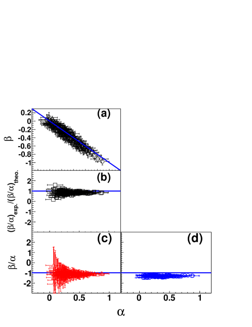
Figure 1: (a) $\beta(N)$ vs $\alpha(Z)$ is plotted for N=Z=7. Line indicates the locus $\beta(N)=-\alpha(Z)$; (b)ratio of $\beta(N)/\alpha(Z)$ data to theoretical Eq.(5) (open squares); (c)$\beta(N)/\alpha(Z)$ vs. $\alpha(Z)$ from data (open triangles); (d)the analytical prediction Eq.(5) (open circles) to compare with data.

In part a of Figure 1 we have plotted $\beta(N)$ vs $\alpha(Z)$. As seen in the figure, the relation $\alpha(Z)\sim-\beta(N)$ is observed for $\alpha(Z)\leq 0.5$ and may deviate slightly at the larger $\alpha(Z)$ values. Those larger values are associated with the largest N/A values for the compound system. In the bottom part of the figure, these values on the left are compared to predictions of Eq.(5) on the right with the assumptions that Z/A is that of the compound system. We note that the experimental values tend to be significantly closer to -1 than the calculated values. Except at the low experimental values of $\alpha(Z)$ where the scatter is significant, the experimental values for $\beta(N)/\alpha(Z)$ are about $20\%$ lower in the absolute value than the model values as indicated by the ratio of these two quantities also plotted in the middle part of the figure. In order to see the system dependence of $\alpha(Z)$ and $\beta(N)$ values, these values are plotted for separate groups of fissility values in Fig.2. The fissility is defined as $X=\frac{Z_{s}^{2}}{A_{s}}$, where $Z_{s}$ and $A_{s}$ are the charges and masses of the source which we assume to be the compound nucleus for simplicity. We can define a combined fissility parameter between reactions (1) and (2) as $\Sigma X=X_{1}+X_{2}$. Larger (absolute) values of $\alpha(Z)$ and $\beta(N)$ correspond to large values of the $\Sigma X$ parameter. In the figure $\alpha(Z)$ and $\beta(N)$ values are separately plotted for four different ranges of fissility group for the same data set used in Fig.1. We see no systematic correlation with the fissility parameters in the deviation from $\alpha(Z)=-\beta(N)$, which might be suggestive of the fact that the Coulomb force is not so effective for breaking the invoked invariance of the Nuclear Hamiltonian. It would be very interesting to see if Coulomb effects become more important for heavy colliding nuclei such as $U+U$. One should note that a similar result is observed for $\alpha(Z)$ and $\beta(N)$ in other IMFs, when Z and N are the same. One can also use $\alpha$ and $\beta$ values averaged over a range of atomic (or neutron) number, though in this case the averaged numbers depend on the somewhat range selected.

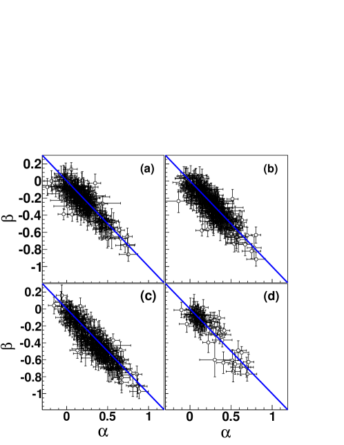
Figure 2: $\beta(N)$ vs $\alpha(Z)$ with $6\leq Z\leq 13$ for different ranges of the fissility parameter. $\Sigma X\leq 60.9$ (top left), $60.9<\Sigma X\leq 72.2$ (top right), $72.2<\Sigma X\leq 83.4$ (bottom left) and $83.4<\Sigma X\leq 94.7$ (bottom right).

While the trend in Figs.1 and 2 is interesting, it is important to note that when the neutron and proton concentrations of the initial excited source are different, two well established trends can act to shift the balance toward symmetric matter and hence to bring the absolute values of the observed $\alpha(Z)$ and $\beta(N)$ parameters closer together. The first is the distillation effect in which early emission of particles favors neutron emission over proton emission serot ; maria . As a result of this early emission the fragmenting system will tend to have a higher symmetry than the initial system. The second is secondary decay of initially excited fragments Marie98 ; Hudan03 which favors a shift toward the evaporation attractor line Charity88 . Thus even if the comparison of primary fragment yields would lead to a significant difference in the two isoscaling parameters the subsequent decay can reduce this difference.

$m$-SCALING

Pursuing the question of phase transitions, we note that we have previously discussed some of the present yield data within the Landau free energy description Bonasera08 . In this approach the ratio of the free energy (per particle) to the temperature is written in terms of an expansion:

$$\frac{F}{T}=\frac{1}{2}am^{2}+\frac{1}{4}bm^{4}+\frac{1}{6}cm^{6}-m\frac{H}{T},$$ (7)

where $m$ is the order parameter, $H$ is its conjugate variable and $a-c$ are fitting parameters. In our case $m=(I/A)$. Notice that the free energy that we have indicated with F includes the chemical potential of neutrons and protons i.e. $AF(m,T)=[G(N,Z)-\mu_{n}N-\mu_{p}Z]$ (compare to Eq.(2)).

We observe that the free energy is even in the exchange of $m\rightarrow-m$ reflecting the invariance of the nuclear forces when exchanging N and Z. This symmetry is violated by the conjugate field $H$ which arises when the source is asymmetric in the chemical composition. We stress that correctly m and H are related to each other through the relation $m=-\frac{\delta F}{\delta H}$.

An immediate consequence of the application of the Landau expression of Eq.(7) in the Modified Fisher Model is that it brings a scaling law for m=0 isotopes. Since F(m=0,T)=0, for any T, the yield in Eq.(2) is given as

$${Y(N,Z)=Y_{0}A^{-\tau},}$$ (8)

for all reactions.

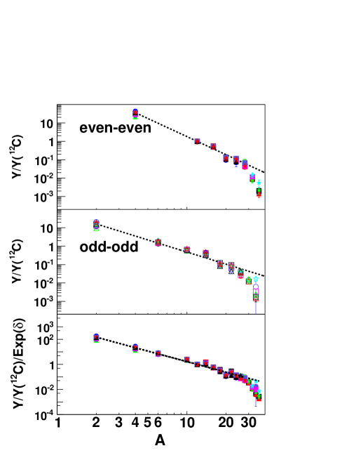
Figure 3: Yield ratio of m=0 isotopes vs A. The yield is normalized to that of ${}^{12}C$. Data from all 18 reaction systems studied in this experiment. (top) even-even isotopes. (middle) odd-odd isotopes are plotted. (bottom) pairing corrected yield, Y(N,Z)/exp($\delta$), are plotted for all m=0 isotopes. Lines in each figure are linear fitted ones. $\tau$ values are 3.3, 2.2 and 2.8 from the top to bottom. $a_{p}/T$ =2.2 is used in the bottom.

In Fig.3, yield ratios for m=0 isotopes are separately plotted as a function of A for even-even (top) and odd-odd (middle) isotopes for all 18 reactions studied here. In order to eliminate the effect of the constant in Eq.(2), which are slightly different in each reaction system, the yield is normalized to that of the ¹²C in each reaction. As seen in the figure, the yields from the different reactions are indeed scaled well with A up to A $\sim$ 30 when even-even and odd-odd isotopes are plotted separately. One should note that data points for a given A represent all 18 different reactions in the figure. The slope difference between even-even and odd-odd isotopes can be naturally attributed to the pairing effect. However a large pairing effect is expected only at a low temperature, because it is related to the shell effect. On the other hand the emitting sources of these isotopes are expected to be at a high temperature. Ricciardi et al. have given a possible explanation for this observation Ricciardi04 ; Ricciardi05 . According model simulations which they have performed the experimentally observed pairing effect is attributed to the last chance particle decay of the excited fragments during their cooling. This hypothesis is also supported by our model simulations presented in a separate paper huang10 . In order to take into account the pairing effect, data for even-even and odd-odd isotopes were simultaneously fitted by the following equation,

$$Y(N,Z)=Y_{0}A^{\tau}exp(\delta/T),$$ (9)

$$\delta(N,Z)=\left\{\begin{array}[]{ll}a_{p}/A^{1/2}&(\textrm{odd-odd})\\ 0&(\textrm{even-odd})\\ -~{}a_{p}/A^{1/2}&(\textrm{even-even}).\end{array}\right.$$ (13)

and the parameters $\tau$ and $a_{p}/T$ values was extracted. Using these extracted parameters, the experimental yield was divided by the exponent in Eq.(9) as factor. The results are plotted in the bottom of the figure for all isotopes with m=0. The extracted $\tau$ value is 2.8 which is larger than the normal critical exponent 2.3. This difference may reflect either the temperature of the emitting source is below the critical temperature or that the secondary decay processes modify the value.

Because of the symmetries of the free energy when we take the ratio between two different systems, $presumably$ at the same temperature $T$ and density $\rho$, all $even$ order terms in $m$ cancel out while the $odd$ terms remain. Those terms depend on the $external$ field $H/T$. Taking the ratio between two systems as in Eq.(2) we easily obtain:

$$R_{12}(m)=Cexp(\Delta H/TmA),$$ (14)

where $\Delta H/T=H_{1}/T-H_{2}/T$. We can fix the constant C by dividing each experimental yield by the ${}^{12}C$ yield following in ref. Bonasera08 . The goal is to get $C\rightarrow 1$ for reasons that will become clear below. Comparing the latter equation with Eq.(1) we obtain: $\Delta H/TmA=\alpha N+\beta Z$ i.e. $\alpha=-\beta=\frac{\Delta H}{T}$. As shown in Fig.1, for the comparison for isotopes of a given Z with isotones having N equal to that Z, this relation appears to be satisfied. The relation is valid more in general, and in fact we could write the chemical potentials of neutrons and protons as:

$$\mu_{n}N+\mu_{p}Z=\mu A+HmA,$$ (15)

from this relation it follows that:

$$2H=\mu_{n}-\mu_{p};2\mu=\mu_{n}+\mu_{p}.$$ (16)

All these relations show that if $m$ is an order parameter then $\alpha=-\beta=\Delta H/T$.

Figure 4: Experimental ratios vs m for isotopes with $6\leq Z\leq 13$ for (a) $\frac{{}^{64}Ni^{232}Th}{{}^{70}Zn^{197}Au}$, (b)$\frac{{}^{64}Ni^{112}Sn}{{}^{64}Ni^{58}Ni}$, (c)$\frac{{}^{64}Ni^{124}Sn}{{}^{64}Ni^{64}Ni}$, (d)$\frac{{}^{64}Ni^{197}Au}{{}^{64}Ni^{112}Sn}$, (e)$\frac{{}^{64}Ni^{124}Sn}{{}^{70}Zn^{58}Ni}$ and (f)$\frac{{}^{64}Ni^{124}Sn}{{}^{70}Zn^{112}Sn}$ respectively at $40MeV/A$. The lines are the results of a linear fit according to Eq.(17).

The external field is given by the difference of chemical potentials between neutrons and protons of the emitting system as expected. ¿From Eq.(14) we can obtain the difference between the free energies (or alternatively the external fields) as:

$$\frac{-ln(R_{12}(m))}{A}=\Delta H/Tm+constant.$$ (17)

Thus a plot of $-ln(R)/A$ versus m should give a linear relation whose slope is given by $\Delta H/T$. This linear relation is demonstrated in Figs.1 and 2 where such a plot is obtained for different colliding systems for the isotopes in the selected range of Z. In thatgiven range $\alpha(Z)$ increases about 50% on average chen ; huang10 . As discussed in references chen ; huang10 , the observed fragment Z (or N) dependence of the isoscaling parameters is mainly established during the statistical cooling of the excited fragments. In fact it has been demonstrated that $\alpha(Z)$ parameter extracted from the primary fragments of the AMD simulations shows no significant fragment Z dependence. It should be noted that it is important to normalize the distribution ( for instance to ${}^{12}C$ ) as we have done in order that the normalizing constant in front of the yield in Eq.(14) is one. If not this will carry a $\frac{1}{A}$ term which might violate the scaling. Overall the scaling is satisfied for this set of data as seen in Fig.4. Compared to ’traditional’ isoscaling where a fit is performed for each detected charge $Z$ (or each $N$) we see that all the data collapse into one curve.

We can further elucidate the role of the external field $H/T$ writing the Landau expansion and ’shifting’ the order parameter by $m_{s}$ which is the position of the minimum of the free energy. Such a position depends on the neutron to proton concentration of the source Bonasera08 . Thus

$$\frac{F}{T}=\frac{1}{2}a(m-m_{s})^{2}+\frac{1}{4}b(m-m_{s})^{4}+\frac{1}{6}c(m-m_{s})^{6}.$$ (18)

Comparing to Eq.(7) we easily obtain

$$\frac{H}{T}=(a+bm^{2}+cm^{4})m_{s}+(\frac{1}{2}\frac{a}{m}+\frac{3}{2}bm+\frac{5}{2}cm^{3})m_{s}^{2}+O(m_{s}^{4})...,$$ (19)

thus $H$ depends on the source isospin concentration though the parameter $a,b,c$ which are terms of the free energy. We stress that these terms refer to the free energy and $not$ to the internal symmetry energy. If b and c are of comparable magnitude to parameter a, then taking terms of a, Eq.(19) can be further simplified as

$$\frac{H}{T}=-am_{s}+\frac{1}{2}a\frac{m_{s}^{2}}{m}+O(m_{s}^{4})...,$$ (20)

II Reconciliation of the two approaches

Standard isoscaling results have been derived under a general grand canonical approach Ono03 ; Tsang01 ; Botvina02 . The Landau approach should be equivalent to it under certain conditions. Experimentally the b and c values have not been established because all isotopes identified in the present data have m $<$ 0.5 except for nucleons. In the case that b and c are of comparable magnitude to parameter a, which is assumed in the derivation of eq.(20), we easily obtain:

$$\frac{\Delta H}{T}mA=a\Delta m_{s}(N-Z)-\frac{1}{2}a(m^{2}_{s1}-m^{2}_{s2})A=\alpha N+\beta Z$$ (21)

which introduces a volume term. Equating similar terms we get:

$$\alpha=a\Delta m_{s}-\frac{1}{2}a(m^{2}_{s1}-m^{2}_{s2})$$ (22)

where $\Delta m_{s}=m_{s1}-m_{s2}$. It is straightforward to demonstrate the equivalence of the last equation to eq.(3) derived from the grand canonical approach. In particular we get:

$$\alpha+\beta=-a(m^{2}_{s1}-m^{2}_{s2})$$ (23)

which shows that the two approaches are equivalent and that $m$ is an order parameter if $\alpha+\beta=0$ i.e. neglecting $O(m_{s}^{2})$ terms in the external field. In figure (5) we plot $\alpha+\beta$ vs. $m^{2}_{s1}-m^{2}_{s2}$, unfortunately the error bars are rather large but we can see a systematic deviation from zero as expected from eq.(23) for large differences in concentration.

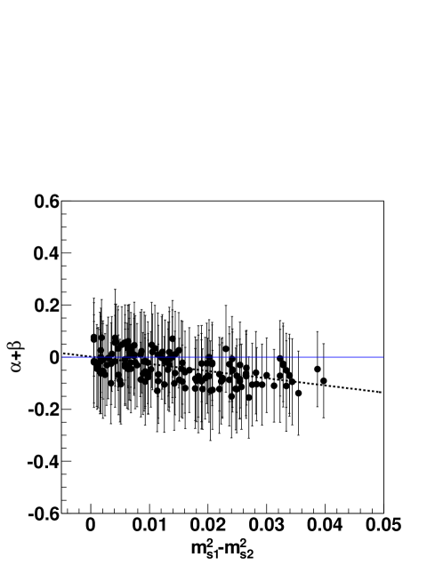
Figure 5: $\alpha(Z)+\beta(N)$ vs the difference (solid circles) in concentration for the two reaction systems for the case of Z=N=7. The dotted line is the result of a linear fit.

This indicates that, at the level of sensitivity so far acheived with data of this type the presence of higher order terms in m is difficult to quantify. Thus, within the error bars, $m$ could be considered an order parameter when relatively neutron (or proton) rich sources are considered. In particular, phase transitions in finite systems could be studied using the same language of macroscopic systems i.e., ’turning on and off’ an external field Bonasera08 .

SUMMARY

In conclusion, in this paper we have discussed scaling of ratios of yields from different colliding systems under similar physical control parameters, i.e. density and temperature. A careful and precise determination of isotopic yields is needed in order to see the features of the system near the phase transition. There is an order parameter, m, given by the difference in neutron and proton concentrations of the detected fragments which leads to an expected isoscaling relation, a direct consequence of the restored symmetry of the nuclear Hamiltonian when exchanging neutrons with protons. The data suggest that the Coulomb field may not significantly violate such a symmetry. The existence of m-scaling might be a signature for near criticality of the fragmenting system. Other properties of the ’rich’ nuclear Hamiltonian, such as pairing, appear to result in small violations of the scaling. This is an interesting physical aspect which deserves further and deep investigation both theoretically and experimentally. Also, it would be interesting to search for m-scaling violations in heavily charged colliding systems such as U+U. The absence of a violation in these cases would suggest that densities and deformations of the fragments are such that the effect of Coulomb is significantly reduced. Studies of the other extreme case of very exotic colliding systems would be also be valuable to probe the effects of high ’external’ field on the phase transition. The atomic nucleus constitutes a formidable laboratory to test our knowledge and understanding of phase transitions in a finite system and offers a unique possibility for different quantum aspects similar to other bosons and fermion mixtures.

A major consideration in the interpretation of the results presented in this paper is the effect of the secondary decay process. In the experiments excited fragments cool down to the ground state before they are detected. The reconstruction of the primary fragments from the experimentally observed IMFs and associated particles is not straightforward, since multiple excited primary fragments may be simultaneously produced in multifragmentation reactions making the unambiguous identification of the primary fragment distribution difficult. Indeed a major goal of the experiments from which the present isoscaling data are taken was to employ fragment-particle correlation measurements to reconstruct the primary fragment distribution. The correlation data are still being analyzed Wada05 .

- (1) R. W. Minich et al., Phys. Lett. B118, 458 (1982).
- (2) A. Bonasera et al., Rivista Nuovo Cimento, 23 (2000) 1.
- (3) A. Bonasera et al., Phys. Rev. Lett. 101, 122702 (2008) and in preparation.
- (4) H. S. Xu et al., Phys. Rev. Lett. 85, 4, (2000).
- (5) M. B. Tsang et al., Phys. Rev. C64, 054615 (2001).
- (6) A.S. Botvina, O. V. Lozhkin and W. Trautmann, Phys. Rev. C65, 044610 (2002).
- (7) A. Ono et al., Phys. Rev. C68, 051601(R) (2003).
- (8) Z.Chen et al., arXiv:1002.0319 [nucl-ex] 1Feb2010.
- (9) M.Huang et al., arXiv:1001.3621 [nucl-ex] 22Jan2010.
- (10) A. Ono, et al., Phys. Rev. C70, 041604(R) (2004).
- (11) M. V. Ricciardi et al., Nucl. Phys. A733 (2004) 299.
- (12) M. V. Ricciardi et al., Nucl. Phys. A749 (2005) 122c.
- (13) H. Muller and B. D. Serot, Phys. Rev. C52 (1995) 2072.
- (14) V.Baran et al., Phys.Rep.410(2005)335. Eur. Phys. J.A30,203 (2006). Cyclotron Institute, Texas A&M University, (2005), II-3, unpublished. DataTables 46, 1 (1990).
- (15) N. Marie et al., Phys. Rev. C58, 256 (1998).
- (16) S. Hudan et al., Phys. Rev. C76, 064613 (2003) 53, 501 (2004).
- (17) R. J. Charity et al., Nucl. Phys. A483, 371 (1988).
- (18) K. Huang, Statistical Mechanics, second edition, ch.16-17, J. Wiley and Sons, New York, 1987.
- (19) R.Wada et al., annual report of the Cyclotron Institute, Texas AM University, (2005), II-3, unpublished. One can find the article in the web page :http://cyclotron.tamu.edu/publications.html.