Theory of orbital magnetoelectric response

Abstract

We extend the recently-developed theory of bulk orbital magnetization to finite electric fields, and use it to calculate the orbital magnetoelectric response of periodic insulators. Working in the independent-particle framework, we find that the finite-field orbital magnetization can be written as a sum of three gauge-invariant contributions, one of which has no counterpart at zero field. The extra contribution is collinear with and explicitly dependent on the electric field. The expression for the orbital magnetization is suitable for first-principles implementations, allowing to calculate the magnetoelectric response coefficients by numerical differentiation. Alternatively, perturbation-theory techniques may be used, and for that purpose we derive an expression directly for the linear magnetoelectric tensor by taking the first field-derivative analytically. Two types of terms are obtained. One, the ‘Chern-Simons’ term, depends only on the unperturbed occupied orbitals and is purely isotropic. The other, ‘Kubo’ terms, involve the first-order change in the orbitals and give isotropic as well as anisotropic contributions to the response. In ordinary magnetoelectric insulators all terms are generally present, while in strong $Z_{2}$ topological insulators only the Chern-Simons term is allowed, and is quantized. In order to validate the theory we have calculated under periodic boundary conditions the linear magnetoelectric susceptibility for a 3-D tight-binding model of an ordinary magnetoelectric insulator, using both the finite-field and perturbation-theory expressions. The results are in excellent agreement with calculations on bounded samples.

1 Introduction

In insulating materials in which both spatial inversion and time-reversal symmetries are broken, a magnetic field ${\bi B}$ can induce a first-order electric polarization ${\bi P}$, and conversely an electric field ${\boldsymbol{\mathcal{E}}}$ can induce a first-order magnetization ${\bi M}$ [1, 2]. This linear magnetoelectric (ME) effect is described by the susceptibility tensor

$$\alpha_{da}=\left.\frac{\partial P_{d}}{\partial B_{a}}\right|_{{\bi B}=0}=\left.\frac{\partial M_{a}}{\partial\mathcal{E}_{d}}\right|_{{\boldsymbol{\mathcal{E}}}=0}$$ (1)

where indices label spatial directions. This tensor can be divided into a “frozen-ion” contribution that occurs even when the ionic coordinates are fixed, and a “lattice-mediated” contribution corresponding to the remainder. Each of these two contributions can be decomposed further according to whether the magnetic interaction is associated with spins or orbital currents, giving four contributions to $\alpha$ in total.

All of those contributions, except the frozen-ion orbital one, are relatively straightforward to evaluate, at least in principle, and ab initio calculations have started to appear. For example, the lattice-mediated spin-magnetization response was calculated in [3] for Cr₂O₃ and in [4] for BiFeO₃ (including the strain deformation effects that are present in the latter), and calculations based on the converse approach (polarization response to a Zeeman field) were recently reported [5]. One generally expects the lattice-mediated couplings to be larger than the frozen-ion ones, and insofar as the spin-orbit interaction can be treated perturbatively, interactions involving spin magnetization are typically larger than the orbital ones. However, we shall see that there are situations in which the spin-orbit interaction cannot be treated perturbatively, and in which the frozen-ion orbital contribution is expected to be dominant. Therefore, it is desirable to have a complete description which accounts for all four contributions.

The frozen-ion orbital contribution is, in fact, the one part of the ME susceptibility for which there is at present no satisfactory theoretical or computational framework, although some progress towards that goal was made in two recent works[6, 7]. Following Essin et al. [7] we refer to it as the “orbital magnetoelectric polarizability” (OMP). For the remainder of this paper, we will focus exclusively on this contribution to (1), and shall denote it simply by $\alpha$. Accordingly, the symbol ${\bi M}$ will be used henceforth for the orbital component of the magnetization.

The question we pose to ourselves is the following: what is the quantum-mechanical expression for the tensor $\alpha$ of a generic three-dimensional band insulator? We note that the conventional perturbation-theory expression for $\alpha$ [8, 9] does not apply to Bloch electrons, as it involves matrix elements of unbounded operators. The proper expressions for ${\bi P}$ [10] and ${\bi M}$ [11, 12, 13, 14] in periodic crystals have been derived, but so far only at ${\bi B}=0$ and ${\boldsymbol{\mathcal{E}}}=0$ respectively. The evaluation of equation (1) remains therefore an open problem.

Phenomenologically, the most general form of $\alpha$ is a $3\times 3$ matrix where all nine components are independent. Dividing it into traceless and isotropic parts, the latter is conveniently expressed in terms of a single dimensionless parameter $\theta$ as

$$\alpha^{\theta}_{da}=\frac{\theta e^{2}}{2\pi hc}\delta_{da}.$$ (2)

The presence of an isotropic ME coupling is equivalent to the addition of a term proportional to $\theta{\boldsymbol{\mathcal{E}}}\cdot{\bi B}$ to the electromagnetic Lagrangian. Such a term describes “axion electrodynamics” [15] and (2) may therefore also be referred to as the “axion OMP.” The electrodynamic effects of the axion field are elusive (in fact, the very existence of $\alpha^{\theta}$ was debated until recently: see [16, 17] and references therein). For example, in a finite, static sample cut from a uniform ME medium those effects are only felt at the surface[15, 18]. In particular, $\alpha^{\theta}$ gives rise to a surface Hall effect [19].

An essential feature of the axion theory is that a change of $\theta$ by $2\pi$ leaves the electrodynamics invariant [15]. The profound implications for the ME response of materials were recognized by Qi et al. [6], and discussed further by Essin et al. [7]. These authors showed that there is a part of the isotropic OMP which remains ambiguous up to integer multiples of $2\pi$ in the corresponding $\theta$ until the surface termination of the sample is specified. For example, a change by $2\pi n$ occurs if the surface is modified by adsorbing a quantum anomalous Hall layer. Hence this particular contribution to $\theta$ can be formulated as a bulk quantity only modulo a quantum of indeterminacy, in much the same way as the electric polarization ${\bi P}$ [10, 20]. A microscopic expression for it was derived in the framework of single-particle band theory by the above authors. It is given by the Brillouin-zone integral of the Chern-Simons form [21] in $k$-space, which is a multivalued global geometric invariant reminiscent of the Berry-phase expression for ${\bi P}$ [10]. We denote henceforth this “geometric” contribution to the OMP as the Chern-Simons OMP (CSOMP).

A remarkable outcome of this analysis is the prediction [6] of a purely isotropic “topological ME effect,” associated with the CSOMP, in a newly-discovered class of time-reversal invariant insulators known as $Z_{2}$ topological insulators [22, 23, 24]. As a result of the multivaluedness of $\theta$, the presence of time-reversal symmetry in the bulk, which takes $\theta$ into $-\theta$, is consistent with two solutions: $\theta=0$, corresponding to ordinary insulators, and $\theta=\pi$, corresponding to strong $Z_{2}$ topological insulators. The latter case is non-perturbative in the spin-orbit interaction, and $\theta=\pi$ amounts to a rather large ME susceptibility (in Gaussian units it is $1/4\pi$ times the fine structure constant, or $\sim$6$\times$10^-4, to be compared with $\sim$1$\times$10^-4 for the total ME response of Cr₂O₃ at low temperature [25]).

It is not clear from these recent works, however, whether the isotropic CSOMP constitutes the full OMP response of a generic insulator. It does appear to do so for the tight-binding model studied in [7], whose ME response was correctly reproduced by the Chern-Simons expression even when the parameters were tuned to break time-reversal and inversion symmetries (i.e., for generic $\theta$ not equal to 0 or $\pi$). On the other hand, other considerations seem to demand additional contributions. For example, it is not difficult to construct tight-binding models of molecular crystals in which it is clear that the OMP cannot be purely isotropic.

In this work we derive, using rigorous quantum-mechanical arguments, an expression for the OMP tensor $\alpha$ of band insulators, written solely in terms of bulk quantities (the periodic Hamiltonian and ground state Bloch wavefunctions, and their first-order change in an electric field). We restrict our derivation to non-interacting Hamiltonians, as the essential physics we wish to describe occurs already at the single-particle level. We find that in crystals with broken time-reversal and inversion symmetries there are, in addition to the CSOMP term discussed in [6, 7], extra terms which generally contribute to both the trace and the traceless parts of $\alpha$.

Our theoretical approach closely mimics one type of ME response experiment: a finite electric field ${\boldsymbol{\mathcal{E}}}$ is applied to a bounded sample, and the (orbital) magnetization is calculated in the presence of the field. Then the thermodynamic limit is taken at fixed field. This key step in the derivation must be done carefully, so that crucial surface contributions are not lost in the process, and here we follow the Wannier-based approach of references [12, 13], adapted to ${\boldsymbol{\mathcal{E}}}\not=0$. Finally the linear response coefficient $\alpha_{da}=\partial M_{a}/\partial\mathcal{E}_{d}$ is extracted in the limit that ${\boldsymbol{\mathcal{E}}}$ goes to zero.

In a concurrent work by Essin, Turner, Moore, and one of us [26] an alternative approach was taken, which is closer in spirit to the calculation in [10] of the change in polarization as an integrated current: the adiabatic current induced in an infinite crystal by a change in its Hamiltonian in the presence of a magnetic field is computed, and then expressed as a total time derivative. The two approaches are complementary and lead to the same expression for $\alpha$, illuminating it from different angles.

The paper is organized as follows. In section 2 we derive the bulk expression for ${\bf M}({\boldsymbol{\mathcal{E}}})$, and reorganize it into three gauge-invariant contributions, one of which yields directly the CSOMP response. The gauge-invariant decomposition of ${\bi M}({\boldsymbol{\mathcal{E}}})$ is done at first in $k$-space for periodic crystals, and then also for bounded samples working in real space. In section 3 we derive a $k$-space formula for the OMP tensor $\alpha$ by taking analytically the field-derivative of ${\bi M}({\boldsymbol{\mathcal{E}}})$. Numerical tests on a tight-binding model of a ME insulator are presented at appropriate places throughout the paper in order to validate the bulk expressions for ${\bi M}({\boldsymbol{\mathcal{E}}})$ and $\alpha$. In A we describe the tight-binding model, as well as technical details on how the various formulas are implemented on a $k$-point grid. B and C contain derivations of certain results given in the main text.

2 Orbital magnetization in finite electric field

2.1 Preliminaries

The orbital magnetization ${\bi M}$ is defined as the orbital moment per unit volume,

$${\bi M}=-\frac{e}{2cV}\sum_{i}\,\langle\psi_{i}|{\bi r}\times{\bi v}|\psi_{i}\rangle.$$ (3)

Here $e>0$ is the magnitude of the electron charge, $V$ is the sample volume, and $|\psi_{i}\rangle$ are the occupied eigenstates. While this expression can be directly implemented when using open boundary conditions, the electronic structure of crystals is more conveniently calculated and interpreted using periodic boundary conditions, in order to take advantage of Bloch’s theorem. This poses however serious difficulties in dealing with the circulation operator ${\bi r}\times{\bi v}$, because of the unbounded and nonperiodic nature of the position operator ${\bi r}$. These subtle issues were fully resolved only recently, with the derivation of a bulk expression for ${\bi M}$ directly in terms of the extended Bloch states [11, 12, 13, 14].

In previous derivations the crystal was taken to be under shorted electrical boundary conditions. We shall extend the derivation given in [12, 13] to the case where a static homogeneous electric field ${\boldsymbol{\mathcal{E}}}$ is present, so that the full Hamiltonian reads

$$\mathcal{H}=\mathcal{H}^{0}+e{\boldsymbol{\mathcal{E}}}\cdot{\bi r}.$$ (4)

The derivation, carried out for an insulator with $N$ valence bands within the independent-particle approximation, involves transforming the set of occupied eigenstates $|\psi_{i}\rangle$ of $\mathcal{H}$ into a set of Wannier-type (i.e., localized and orthonormal) orbitals $|w_{i}\rangle$ and expressing ${\bi M}({\boldsymbol{\mathcal{E}}})$ in the Wannier representation. This is done at first for a finite sample cut from a periodic crystal, and eventually the thermodynamic limit is taken at fixed field.

Before continuing, two remarks are in order. First, the assumption that it is possible to construct well-localized Wannier functions (WFs) spanning the valence bands is only valid if the Chern invariants of the valence bandstructure vanish identically [27]. This requirement is satisfied by normal band insulators as well as by $Z_{2}$ topological insulators, but not by quantum anomalous Hall insulators [28], which thus far remain hypothetical. Second, because of Zener tunnelling, an insulating crystal does not have a well-defined ground state in a finite electric field. Nonetheless, upon slowly ramping up the field to the desired value, the electron system remains in a quasistationary state which is, for all practical purposes, indistinguishable from a truly stationary state. This is the state we shall consider in the ensuing derivation. As discussed in [29, 30], it is Wannier- and Bloch-representable, even though the Hamiltonian (4) is not lattice-periodic.

2.2 $k$-space expression

Our derivation of a $k$-space (bulk) expression for ${\bi M}({\boldsymbol{\mathcal{E}}})$ is carried out mostly in real space, using a Wannier representation. It is only in the last step that we switch to reciprocal space, by expressing the crystalline WFs $|{\bi R}n\rangle$ in terms of the cell-periodic Bloch functions $|u_{n{\bi k}}\rangle$ via [31]

$$|{\bi R}n\rangle=V_{\rm c}\int[\rmd k]\rme^{\rmi{\bi k}\cdot({\bi r}-{\bi R})}|u_{n{\bi k}}\rangle,$$ (5)

where ${\bi R}$ is a lattice vector, $V_{\rm c}$ is the unit-cell volume, $[\rmd k]\equiv\rmd^{3}k/(2\pi)^{3}$, and the integral is over the first Brillouin zone.

We begin with a finite sample immersed in a field ${\boldsymbol{\mathcal{E}}}$, divide it up into an interior region and a surface region, and assign each WF to either one. The boundary between the two regions is chosen in such a way that the fractional volume of the surface region goes to zero as $V\rightarrow\infty$, but deep enough that WFs near the boundary are bulk-like. Following [12, 13], equation (3) for the orbital magnetization can then be rewritten as an interior contribution plus a surface contribution, denoted respectively as the “local circulation” (LC) and the “itinerant circulation” (IC). Remarkably, in the thermodynamic limit both can be expressed solely in terms of the interior-region crystalline WFs, or equivalently, in terms of the bulk Bloch functions, as shown in the above references at ${\boldsymbol{\mathcal{E}}}=0$ and below for ${\boldsymbol{\mathcal{E}}}\not=0$. Specifically, we shall show that

$${\bi M}={\bi M}^{\rm LC}+{\bi M}^{{\rm IC},0}+{\bi M}^{{\rm IC},{\boldsymbol{\mathcal{E}}}},$$ (6a)

where

$$M^{\rm LC}_{a}=-\gamma\epsilon_{abc}\mathrm{Im}\sum_{n}^{N}\,\int[\rmd k]\langle\partial_{b}u_{n{\bi k}}|H^{0}_{\bi k}|\partial_{c}u_{n{\bi k}}\rangle$$ (6b)

is the contribution from the interior WFs,

$$M^{{\rm IC},0}_{a}=-\gamma\epsilon_{abc}\mathrm{Im}\sum_{nm}^{N}\,\int[\rmd k]\langle\partial_{b}u_{n{\bi k}}|\partial_{c}u_{m{\bi k}}\rangle H^{0}_{mn{\bi k}}$$ (6c)

is the part of the surface contribution coming from the zero-field Hamiltonian, and

$$M^{{\rm IC},{\boldsymbol{\mathcal{E}}}}_{a}=-\gamma\epsilon_{abc}\mathrm{Im}\sum_{nm}^{N}\,\int[\rmd k]\langle\partial_{b}u_{n{\bi k}}|\partial_{c}u_{m{\bi k}}\rangle e{\boldsymbol{\mathcal{E}}}\cdot{\bi A}_{mn{\bi k}}$$ (6d)

is the part of the surface contribution coming from the electric field term in the Hamiltonian (4). In the above expressions $\gamma=-e/(2\hbar c)$,

$$H^{0}_{\bi k}=\rme^{-\rmi{\bi k}\cdot{\bi r}}\mathcal{H}^{0}\rme^{\rmi{\bi k}\cdot{\bi r}},$$ (6g)

$$H^{0}_{mn{\bi k}}=\langle u_{m{\bi k}}|H^{0}_{\bi k}|u_{n{\bi k}}\rangle,$$ (6h)

and ${\bf A}_{mn{\bi k}}$ is the Berry connection matrix defined in equation (6n) below.

Having stated the result we now present the derivation, starting with the interior contribution ${\bi M}^{\rm LC}$. Using $[r_{i},r_{j}]=0$, the velocity operator ${\bi v}=(\rmi/\hbar)[\mathcal{H},{\bi r}]$ becomes $(\rmi/\hbar)[\mathcal{H}^{0},{\bi r}]$, so that the circulation operator ${\bi r}\times{\bi v}$ is unaffected by the electric field. It immediately follows that the local circulation part ${\bi M}^{\rm LC}$ is given in terms of the field-polarized states $|u_{n{\bi k}}\rangle$ by the same expression, equation (6b), as was derived in [13] for the zero-field case.

Consider now the contribution ${\bi M}^{\rm IC}={\bi M}^{{\rm IC},0}+{\bi M}^{{\rm IC},{\boldsymbol{\mathcal{E}}}}$ from the surface WFs $|w_{s}\rangle$. For large samples it takes the form [13]

$${\bi M}^{\rm IC}=-\frac{e}{2cN_{\rm c}V_{\rm c}}\sum_{s}^{\rm surf}\,{\bi r}_{s}\times{\bi v}_{s},$$ (6i)

where $N_{\rm c}$ is the number of crystal cells of volume $V_{\rm c}$, ${\bi r}_{s}=\langle w_{s}|{\bi r}|w_{s}\rangle$, and

$${\bi v}_{s}=\langle w_{s}|{\bi v}|w_{s}\rangle=\frac{2}{\hbar}\mathrm{Im}\langle w_{s}|{\bi r}\mathcal{H}|w_{s}\rangle.$$ (6j)

Note that $\mathcal{H}|w_{s}\rangle$ already belongs to the occupied manifold spanned by $P=\sum_{j}^{\rm occ}\,|w_{j}\rangle\langle w_{j}|$, since we assume a (quasi)stationary state. Thus we can insert a $P$ between ${\bi r}$ and $\mathcal{H}$ above, and using (4) we obtain

$${\bi v}_{s}=\sum_{j}^{N}\,\left({\bi v}_{\langle js\rangle}^{0}+{\bi v}_{\langle js\rangle}^{\boldsymbol{\mathcal{E}}}\right),$$ (6k)

where ${\bi v}_{\langle js\rangle}^{0}=(2/\hbar)\mathrm{Im}[{\bi r}_{sj}\mathcal{H}^{0}_{js}]$ is the same as in [12, 13] and ${\bi v}_{\langle js\rangle}^{\boldsymbol{\mathcal{E}}}=(2e/\hbar)\mathrm{Im}[{\bi r}_{sj}({\bi r}_{js}\cdot{\boldsymbol{\mathcal{E}}})]$ is a new term.

The reasoning [12, 13] by which ${\bi M}^{\rm IC}$ can be recast in terms of the bulk WFs $|{\bi R}n\rangle$ relies on the exponential localization of the WFs and on certain properties of ${\bi v}_{\langle js\rangle}^{0}$ (antisymmetry under $j\leftrightarrow s$ and invariance under lattice translations deep inside the crystallite) which are shared by ${\bi v}_{\langle js\rangle}^{\boldsymbol{\mathcal{E}}}$. Hence we can follow similar steps as in those works, arriving at

$$M^{{\rm IC},{\boldsymbol{\mathcal{E}}}}_{a}=\frac{e}{4cV_{\rm c}}\epsilon_{abc}\sum_{\bi R}\sum_{mn}^{N}\,v^{{\boldsymbol{\mathcal{E}}}}_{\langle{\boldsymbol{\it 0}}m,{\bi R}n\rangle,b}R_{c},$$ (6l)

and similarly for $M^{{\rm IC},0}_{a}$ with $v^{0}$ substituting for $v^{{\boldsymbol{\mathcal{E}}}}$. The latter is identical to the expression for $M^{\rm IC}_{a}$ valid at ${\boldsymbol{\mathcal{E}}}=0$ [12, 13], and upon converting to $k$-space becomes (6c).

Let us now turn to $M^{{\rm IC},{\boldsymbol{\mathcal{E}}}}_{a}$ and write (6l) as $(e^{2}/2c\hbar V_{\rm c})\epsilon_{abc}\mathcal{E}_{d}\mathrm{Im}W_{bd,c}$ where

$$W_{bd,c}=\sum_{\bi R}\sum_{mn}^{N}\,\langle{\bi R}n|r_{b}|{\boldsymbol{\it 0}}m\rangle\langle{\boldsymbol{\it 0}}m|r_{d}|{\bi R}n\rangle R_{c}.$$ (6m)

In order to recast this expression as a $k$-space integral it is useful to introduce the $N\times N$ Berry connection matrix

$$A_{mn{\bi k},b}=\rmi\langle u_{m{\bi k}}|\partial_{b}u_{n{\bi k}}\rangle=A_{nm{\bi k},b}^{*},$$ (6n)

where $\partial_{b}\equiv\partial/\partial k_{b}$. It satisfies the relation [31, 32]

$$\langle{\bi R}n|r_{b}|{\boldsymbol{\it 0}}m\rangle=V_{c}\int[\rmd k]A_{nm{\bi k},b}\rme^{\rmi{\bi k}\cdot{\bi R}}.$$ (6o)

We also need

$$R_{c}\langle{\bi R}n|r_{d}|{\boldsymbol{\it 0}}m\rangle=\rmi V_{c}\int[\rmd k](\partial_{c}A_{nm{\bi k},d})\rme^{\rmi{\bi k}\cdot{\bi R}},$$ (6p)

which follows from (6o). Using these two relations, (6m) becomes

$$W_{bd,c}=\rmi V_{c}\sum_{mn}^{N}\int[\rmd k]A_{mn{\bi k},d}\partial_{c}A_{nm{\bi k},b},$$ (6q)

and we arrive at (6d).

The sum of equations (6b)–(6d) gives the desired $k$-space expression for ${\bi M}({\boldsymbol{\mathcal{E}}})$. In the limit ${\boldsymbol{\mathcal{E}}}\rightarrow 0$ the term ${\bi M}^{{\rm IC},{\boldsymbol{\mathcal{E}}}}$ vanishes, and equation (31) of [13] is recovered.

We have implemented (6b)–(6d) for the tight-binding model of A. Since for small electric fields ${\bi M}({\boldsymbol{\mathcal{E}}})$ differs only slightly from ${\bi M}(0)$, in order to observe the effect of the electric field we consider differences in magnetization rather than the absolute magnetization. Therefore, in all our numerical tests we evaluated the OMP tensor $\alpha_{da}$. With the help of (6b)–(6d) we calculated it as $\Delta M_{a}/\Delta\mathcal{E}_{d}$, using small fields $\mathcal{E}_{d}=\pm 0.01$. We then repeated the calculation on finite samples cut from the bulk crystal, using (3) in place of (6b)–(6d). Figure 1 shows the value of the $zz$ and $zy$ components of $\alpha$ plotted as a function of the parameter $\varphi$, the phase of one of the complex hopping amplitudes (see A for details). The very precise agreement between the solid and dashed lines confirms the correctness of the $k$-space formula. The same level of agreement was found for the other components of $\alpha$.

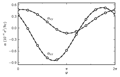
Figure 1: The $zz$ and $zy$ components of the OMP tensor $\alpha$ of the tight-binding model described in A, as a function of the parameter $\varphi$. The two lower bands are treated as occupied. Solid line: extrapolation from finite-size samples using numerical differentiation of the finite-field magnetization calculated from (3). Dashed line: numerical differentiation of the finite-field magnetization calculated using (6b)–(6d) discretized on a $k$-space grid. Open circles: linear-response calculation in $k$-space using discretized versions of (6ahaoaua)–(6ahaoau).

2.3 Gauge-invariant decomposition

2.3.1 Periodic crystals

Equation (6a) for ${\bi M}({\boldsymbol{\mathcal{E}}})$ is valid in an arbitrary gauge, that is, the sum of its three terms given by (6b)–(6d) – but not each term individually – remains invariant under a unitary transformation

$$|u_{n{\bi k}}\rangle\rightarrow\sum_{m}^{N}\,|u_{m{\bi k}}\rangle U_{mn{\bi k}}$$ (6r)

among the valence-band states at each ${\bi k}$. In order to make the gauge invariance of (6a) manifest, it is convenient to first manipulate it into a different form, given in terms of certain canonical objects which we now define. We begin by introducing the covariant $k$-derivative of a valence state [30],

$$|\widetilde{\partial}_{b}u_{n{\bi k}}\rangle=Q_{\bi k}\,|\partial_{b}u_{n{\bi k}}\rangle,$$ (6s)

where $Q_{\bi k}=1-P_{\bi k}$ and

$$P_{\bi k}=\sum_{j=1}^{N}|u_{j{\bi k}}\rangle\langle u_{j{\bi k}}|.$$ (6t)

The covariant and ordinary derivatives are related by

$$|\partial_{b}u_{n{\bi k}}\rangle=|\widetilde{\partial}_{b}u_{n{\bi k}}\rangle-\rmi\sum_{m}^{N}A_{mn{\bi k},b}|u_{m{\bi k}}\rangle.$$ (6u)

The generalized metric-curvature tensor is [31]

$$F_{nm{\bi k},bc}=\langle\widetilde{\partial}_{b}u_{n{\bi k}}|\widetilde{\partial}_{c}u_{m{\bi k}}\rangle=F_{mn{\bi k},cb}^{*}.$$ (6v)

Viewed as an $N\times N$ matrix over the band indices, $F$ is gauge-covariant, changing as

$$F_{nm{\bi k},bc}\rightarrow\left(U_{\bi k}^{\dagger}F_{{\bi k},bc}U_{\bi k}\right)_{nm}$$ (6w)

under the transformation (6r). We also note the relation

$$\langle\partial_{b}u_{n{\bi k}}|\partial_{c}u_{m{\bi k}}\rangle=F_{nm{\bi k},bc}+(A_{{\bi k},b}A_{{\bi k},c})_{nm}.$$ (6x)

We shall make use of two more gauge-covariant objects,

$$H^{0}_{nm{\bi k},b}=\rmi\langle u_{n{\bi k}}|H^{0}_{\bi k}|\widetilde{\partial}_{b}u_{m{\bi k}}\rangle$$ (6y)

and

$$H^{0}_{nm{\bi k},bc}=\langle\widetilde{\partial}_{b}u_{n{\bi k}}|H^{0}_{\bi k}|\widetilde{\partial}_{c}u_{m{\bi k}}\rangle,$$ (6z)

which enter the relation

$$\langle\partial_{b}u_{n{\bi k}}|H^{0}_{\bi k}|\partial_{c}u_{m{\bi k}}\rangle=H^{0}_{nm{\bi k},bc}+\left[A_{{\bi k},b}H^{0}_{{\bi k},c}+\left(H^{0}_{{\bi k},b}\right)^{\dagger}A_{{\bi k},c}+A_{{\bi k},b}H^{0}_{\bi k}A_{{\bi k},c}\right]_{nm}.$$ (6aa)

Coming back to equations (6a)–(6d), for $M^{\rm LC}_{a}$ we use (6aa) and for $M^{\rm IC}_{a}$ we use (6x), leading to

$$M_{a}=-\gamma\epsilon_{abc}\int[\rmd k]\,\mathrm{Im\,}\tr\Big{[}H^{0}_{bc}+2A_{b}H^{0}_{c}+H^{0}F_{bc}+e\mathcal{E}_{d}A_{d}F_{bc}+e\mathcal{E}_{d}A_{d}A_{b}A_{c}\Big{]},$$ (6ab)

where “tr” denotes the electronic trace over the occupied valence bands and we have dropped the subscript ${\bi k}$. The second term can be rewritten using

$$H^{0}_{nm,c}=-e\mathcal{E}_{d}F_{nm,dc}.$$ (6ac)

(To obtain this relation start from the generalized Schrödinger equation satisfied by the valence states at ${\boldsymbol{\mathcal{E}}}\not=0$ [33],

$$H^{0}|u_{n}\rangle=\sum_{m}^{N}\,(H^{0}_{mn}+e{\boldsymbol{\mathcal{E}}}\cdot{\bi A}_{mn})|u_{m}\rangle-\rmi e\mathcal{E}_{d}|\partial_{d}u_{n}\rangle,$$ (6ad)

and multiply through by $\langle\widetilde{\partial}_{c}u_{m}|$.)

Let us define the quantities

$${\widetilde{M}}^{\rm LC}_{a}=-\gamma\epsilon_{abc}\int[\rmd k]\mathrm{Im\,}\tr\left[H^{0}_{bc}\right],$$ (6ae)

$$\widetilde{M}^{\rm IC}_{a}=-\gamma\epsilon_{abc}\int[\rmd k]\mathrm{Im\,}\tr\left[H^{0}F_{bc}\right],$$ (6af)

and

$$M^{\rm CS}_{a}=-e\gamma\epsilon_{abc}\mathcal{E}_{d}\int[\rmd k]\mathrm{Im\,}\tr\bigl{[}2A_{b}F_{cd}+F_{bc}A_{d}+A_{b}A_{c}A_{d}\bigr{]}.$$ (6ag)

The total magnetization is given by their sum

$$M_{a}={\widetilde{M}}^{\rm LC}_{a}+\widetilde{M}^{\rm IC}_{a}+M^{\rm CS}_{a}.$$ (6aha)

Referring to (6v) and (6z) the first two terms read, in a more conventional notation,

$${\widetilde{M}}^{\rm LC}_{a}=-\gamma\epsilon_{abc}\int[\rmd k]\sum_{n}^{N}\,\mathrm{Im}\langle\widetilde{\partial}_{b}u_{n{\bi k}}|H^{0}_{\bi k}|\widetilde{\partial}_{c}u_{n{\bi k}}\rangle$$ (6ahb)

and

$$\widetilde{M}^{\rm IC}_{a}=-\gamma\epsilon_{abc}\int[\rmd k]\sum_{nm}^{N}\,\mathrm{Im}\left(H^{0}_{nm{\bi k}}\langle\widetilde{\partial}_{b}u_{m{\bi k}}|\widetilde{\partial}_{c}u_{n{\bi k}}\rangle\right).$$ (6ahc)

These are the only terms that remain in the limit $${\boldsymbol{\mathcal{E}}}\rightarrow 0 {\boldsymbol{\mathcal{E}}}$$, in agreement with equation (43) of [13]. At finite field they depend on implicitly via the wavefunctions.

We now show that the term ${\bi M}^{\rm CS}$, which gathers all the contributions with an explicit dependence on ${\boldsymbol{\mathcal{E}}}$, can be recast as

$$M^{\rm CS}_{a}=e\gamma\mathcal{E}_{a}\int[\rmd k]\epsilon_{ijk}\tr\left[A_{i}\partial_{j}A_{k}-\frac{2\rmi}{3}A_{i}A_{j}A_{k}\right].$$ (6ahd)

To do so it is convenient to introduce the Berry curvature tensor

$$\Omega_{nm,ab}=\rmi F_{nm,ab}-\rmi F_{nm,ba}=-\Omega_{nm,ba},$$ (6ahai)

where $F_{nm,ab}$ was defined in (6v). A few lines of algebra show that

$$\Omega_{nm,ab}=\partial_{a}A_{nm,b}-\partial_{b}A_{nm,a}-\rmi[A_{a},A_{b}]_{nm}.$$ (6ahaj)

In order to go from (6ag) to (6ahd), use (6ahai) to write $\mathrm{Im\,}\tr[F_{bc}A_{d}]$ as $-\frac{1}{2}\tr[A_{d}\Omega_{bc}]$ and $-2\mathrm{Im\,}\tr[A_{b}F_{dc}]$ as $\tr[A_{b}\Omega_{dc}]$, and then replace $\Omega_{nm,bc}$ in these expressions with $\epsilon_{abc}\Omega_{nm,a}$, where $\Omega_{nm,a}=\frac{1}{2}\epsilon_{abc}\Omega_{nm,bc}$ is the Berry curvature tensor written in axial-vector form. This leads to

$$M^{\rm CS}_{a}=e\gamma\int[\rmd k]\big{(}\mathcal{E}_{a}\tr[\boldsymbol{\Omega}\cdot{\bi A}]-\mathcal{E}_{d}\epsilon_{abc}\mathrm{Im\,}\tr[A_{b}A_{c}A_{d}]\big{)}.$$ (6ahak)

The first term is parallel to the field, and can be rewritten with the help of (6ahaj):

$$\tr[\boldsymbol{\Omega}\cdot{\bi A}]=\epsilon_{ijk}\tr[A_{i}\partial_{j}A_{k}-\rmi A_{i}A_{j}A_{k}].$$ (6ahal)

While not immediately apparent, the second term in (6ahak) also points along the field. To see this, write

$$\sum_{bcd}\,\mathcal{E}_{d}\epsilon_{abc}\mathrm{Im\,}\tr[A_{b}A_{c}A_{d}]=\mathcal{E}_{a}\sum_{bc}\,\epsilon_{abc}\mathrm{Im\,}\tr[A_{a}A_{b}A_{c}]+\sum_{d\not=a}\sum_{bc}\,\epsilon_{abc}\mathrm{Im\,}\tr[A_{b}A_{c}A_{d}],$$ (6aham)

where we suspended momentarily the implied summation convention. The last term vanishes because the factor $\epsilon_{abc}$ forces $d\not=a$ to equal either $b$ or $c$, producing terms such as $\mathrm{Im\,}\tr[A_{b}A_{b}A_{c}]$ which vanish identically as $A_{b}$ is Hermitian. Rewriting $\mathcal{E}_{a}\sum_{bc}\,\epsilon_{abc}\mathrm{Im\,}\tr[A_{a}A_{b}A_{c}]$ as $(\mathcal{E}_{a}/3)\sum_{ijk}\epsilon_{ijk}\mathrm{Im\,}\tr[A_{i}A_{j}A_{k}]$ and restoring the summation convention, we arrive at (6ahd).

Equations (6ahb)–(6ahd), which constitute the main result of this section, are separately gauge-invariant. For $\widetilde{{\bi M}}^{\rm LC}$ and $\widetilde{{\bi M}}^{\rm IC}$ this is apparent already from (6ae) and (6af), whose integrands are gauge-invariant, being traces over gauge-covariant matrices. In contrast, equation (6ahd) for ${\bi M}^{\rm CS}$ only becomes invariant after taking the integral on the right-hand-side over the entire Brillouin zone (the integrand being familiar from differential geometry as the Chern-Simons 3-form [34, 21]).

The Chern-Simons contribution (6ahd) has several remarkable features: (i) as already noted, it is perfectly isotropic, remaining parallel to ${\boldsymbol{\mathcal{E}}}$ for arbitrary orientations of ${\boldsymbol{\mathcal{E}}}$ relative to the crystal axes; (ii) being isotropic, it vanishes in less than three dimensions, which intuitively can be understood because already in two dimensions polarization must be in the plane of the system and magnetization must be out of the plane; (iii) for $N>1$ valence bands it is a multivalued bulk quantity with a quantum of arbitrariness $(e^{2}/hc)\mathcal{E}_{a}$, a fact that is connected with the possibility of a cyclic adiabatic evolution that would change (6ahaoaua) below for $\theta$ by $2\pi$ [6].

We have repeated the calculation of the OMP presented in figure 1 using (6ahb)–(6ahd) instead of (6b)–(6d), finding excellent agreement between them. The electric field derivative of the decomposition (6aha) gives the corresponding decomposition of the OMP tensor (1),

$$\alpha=\widetilde{\alpha}^{\rm LC}+\widetilde{\alpha}^{\rm IC}+\alpha^{\rm CS},$$ (6ahan)

where each term is also gauge-invariant. The $zz$ components of these terms are plotted separately in figure 2.

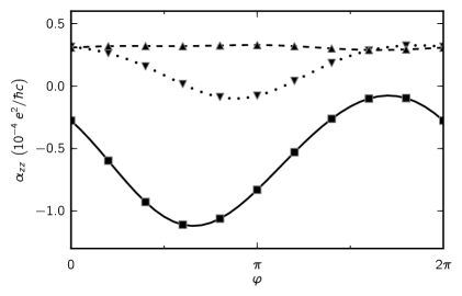
Figure 2: Decomposition of the $\alpha_{zz}$ curve in figure 1 into the gauge-invariant contributions $\widetilde{\alpha}^{\rm LC}_{zz}$ (solid lines), $\widetilde{\alpha}^{\rm IC}_{zz}$ (dashed line), and $\alpha^{\rm CS}_{zz}$ (dotted line), calculated in $k$-space using finite differences in ${\boldsymbol{\mathcal{E}}}$. Symbols denote the same contributions evaluated for bounded samples, also using finite differences.

2.3.2 Finite samples

It is natural to ask whether the gauge-invariant decomposition of the orbital magnetization given in equation (6aha) can be made already for finite samples, before taking the thermodynamic limit and switching to periodic boundary conditions. This has previously been done in the case ${\boldsymbol{\mathcal{E}}}=0$, where ${\bi M}^{\rm CS}=0$ and ${\widetilde{\bi M}}^{\rm LC}$ and $\widetilde{{\bi M}}^{\rm IC}$ take the form [35]

$${\widetilde{M}}^{\rm LC}_{a}=\frac{e}{2\hbar cV}\epsilon_{abc}\mathrm{Im\,}\Tr\,[Pr_{b}Q\mathcal{H}^{0}Qr_{c}]$$ (6ahaoa)

and

$$\widetilde{M}^{\rm IC}_{a}=\frac{e}{2\hbar cV}\epsilon_{abc}\mathrm{Im\,Tr}\,[P\mathcal{H}^{0}Pr_{b}Qr_{c}].$$ (6ahaob)

Here $$P Q=1-P$$ and are the projection operators onto the occupied and empty subspaces, respectively, and “Tr” denotes the electronic trace over the entire Hilbert space. These two expressions, which are manifestly gauge-invariant, remain valid at finite field, reducing to (6ahb) and (6ahc) in the thermodynamic limit.

We now complete this picture for ${\boldsymbol{\mathcal{E}}}\not=0$ by showing that the remaining contribution ${\bi M}^{\rm CS}={\bi M}-{\widetilde{\bi M}}^{\rm LC}-\widetilde{{\bi M}}^{\rm IC}$ can also be written in trace form, as

$$M^{\rm CS}_{a}=-\frac{e^{2}}{3\hbar cV}\mathcal{E}_{a}\epsilon_{ijk}\mathrm{Im\,}\Tr\,[Pr_{i}Pr_{j}Pr_{k}].$$ (6ahaoc)

We first recast the orbital magnetization (3) as

$$M_{a}=-\frac{e}{2cV}\epsilon_{abc}\mathrm{Tr}\,[Pr_{b}v_{c}]=\frac{e}{2\hbar cV}\epsilon_{abc}\mathrm{Im\,}\Tr\,\bigl{[}Pr_{b}\mathcal{H}^{0}r_{c}\bigr{]}$$ (6ahaoap)

and then subtract (6ahaoa) and (6ahaob) from it to find, after some manipulations,

$$M^{\mathrm{CS}}_{a}=-\frac{e}{\hbar cV}\epsilon_{abc}\mathrm{Im\,Tr}\,[Q\mathcal{H}^{0}Pr_{b}Pr_{c}].$$ (6ahaoaq)

Replacing $\mathcal{H}^{0}$ with $\mathcal{H}-e\mathcal{E}_{d}r_{d}$ and using $Q\mathcal{H}P=0$,

$$M^{\rm CS}_{a}=-\frac{e^{2}}{\hbar cV}\epsilon_{abc}\mathcal{E}_{d}\mathrm{Im\,Tr}\,[Pr_{d}Pr_{b}Pr_{c}].$$ (6ahaoar)

The imaginary part of the trace vanishes if any two of the indices $b$, $c$, or $d$ are the same, and therefore $d$ must be equal to $a$. Using the cyclic property we conclude that all non-vanishing terms in the sum over $b$ and $c$ are identical, leading to (6ahaoc). This part of the field-induced magnetization is clearly isotropic, with a coupling strength (see equation (2)) given by

$$\theta^{\rm CS}=-\frac{4\pi^{2}}{3V}\epsilon_{ijk}\mathrm{Im\,}\Tr[Pr_{i}Pr_{j}Pr_{k}].$$ (6ahaoas)

This expression can assume nonzero values because the Cartesian components of the projected position operator $P{\bi r}P$ do not commute [31].

We have used (6ahaoa)–(6ahaoc) to evaluate the OMP contributions $\widetilde{\alpha}^{\rm LC}$, $\widetilde{\alpha}^{\rm IC}$, and $\alpha^{\rm CS}$ for finite samples, finding excellent agreement with the $k$-space calculations using (6ahb)–(6ahd). As an example, the finite-sample results for the $zz$ component are plotted as the symbols in figure 2.

3 Linear-response expression for the OMP tensor

In sections 2.2 and 2.3.1 expressions were given for evaluating ${\bi M}({\boldsymbol{\mathcal{E}}})$ under periodic boundary conditions. Used in conjunction with finite-field ab-initio methods for periodic insulators [36, 29], they allow to calculate the OMP tensor by finite differences. Alternatively, the electric field may be treated perturbatively [33]. With this approach in mind, we shall now take the ${\boldsymbol{\mathcal{E}}}$-field derivative in (1) analytically and obtain an expression for the OMP tensor which is amenable to density-functional perturbation-theory implementation [37]. It should be kept in mind that in the context of self-consistent-field (SCF) calculations the “zero-field” part of the Hamiltonian (4),

$$\mathcal{H}^{0}=-\frac{\hbar^{2}}{2m}\nabla^{2}+V_{\rm SCF}({\bi r}),$$ (6ahaoat)

does depend on ${\boldsymbol{\mathcal{E}}}$ implicitly, through the charge density. As we will see, this dependence gives rise to additional local-field screening terms in the expression for the OMP.

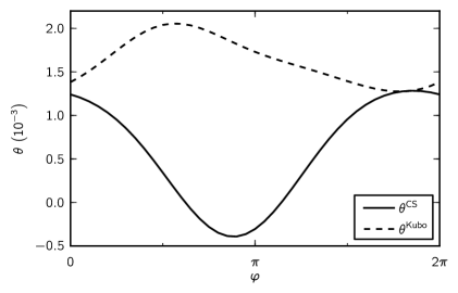
Figure 3: Contributions to the isotropic OMP from the Chern-Simons term $\alpha^{\rm CS}$ and from the Kubo-like terms $\widetilde{\alpha}^{\rm LC}$ and $\widetilde{\alpha}^{\rm IC}$, expressed in terms of the dimensionless coupling strength $\theta$ in (2). Model parameters are the same as for figure 1.

We shall only consider the case where the OMP is calculated for a reference state at zero field, which we indicate by a superscript “0.” Upon inserting (6aha) into (1) we obtain the three gauge-invariant OMP terms in (6ahan). The term $\alpha^{\rm CS}$ is clearly of the isotropic form (2), with

$$\theta^{\rm CS}=-\frac{1}{4\pi}\int\rmd^{3}k\,\epsilon_{ijk}\tr\left[A_{i}^{0}\partial_{j}A_{k}^{0}-\frac{2\rmi}{3}A_{i}^{0}A_{j}^{0}A_{k}^{0}\right].$$ (6ahaoaua)

This is the same expression as obtained previously by heuristic methods [6, 7]. The other two terms were not considered in the previous works. They are

$$\widetilde{\alpha}^{\rm LC}_{da}=\gamma\epsilon_{abc}\int[\rmd k]\,\sum_{n}^{N}\,\mathrm{Im}\Big{(}2\langle\widetilde{\partial}_{b}u^{0}_{n{\bi k}}|(\partial_{c}H^{0}_{\bi k})|\widetilde{\partial}_{D}u_{n{\bi k}}^{0}\rangle$$

$$\;\;\;\;\;\;\;\;\;\;\;\;\;\;\;\;\;\;\;\;\;\;\;\;\;\;\;\;\;\;\;\;\;\;\;\;\;\;\;\;\;-\langle\widetilde{\partial}_{b}u^{0}_{n{\bi k}}|(\partial_{D}H^{0}_{\bi k})|\widetilde{\partial}_{c}u_{n{\bi k}}^{0}\rangle$$ (6ahaoaub)

and

$$\widetilde{\alpha}^{\rm IC}_{da}=\gamma\epsilon_{abc}\int[\rmd k]\,\sum_{mn}^{N}\,\mathrm{Im}\Big{(}2\langle\widetilde{\partial}_{b}u_{n{\bi k}}^{0}|\widetilde{\partial}_{D}u_{m{\bi k}}^{0}\rangle\langle u_{m{\bi k}}^{0}|(\partial_{c}H^{0}_{\bi k})|u_{n{\bi k}}^{0}\rangle$$

$$\;\;\;\;\;\;\;\;\;\;\;\;\;\;\;\;\;\;\;\;\;\;\;\;\;\;\;\;\;\;\;\;\;\;\;\;\;\;\;\,\,-\langle\widetilde{\partial}_{b}u_{n}^{0}|\widetilde{\partial}_{c}u_{m}^{0}\rangle\langle u_{m}^{0}|(\partial_{D}H^{0}_{\bi k})|u_{n}^{0}\rangle\Big{)},$$ (6ahaoauc)

where $\partial_{D}$ denotes the field-derivative $\partial/\partial\mathcal{E}_{d}$ and

$$|\widetilde{\partial}_{D}u_{n{\bi k}}^{0}\rangle\equiv Q_{\bi k}\left.|\partial_{D}u_{n{\bi k}}\rangle\right|_{{\boldsymbol{\mathcal{E}}}=0}$$ (6ahaoauav)

are the first-order field-polarized states projected onto the unoccupied manifold. The terms containing $\partial_{D}H^{0}_{\bi k}$ describe the screening by local fields. They vanish for tight-binding models such as the one in this work, but should be included in self-consistent calculations, in the way described in [37]. We shall sometimes refer to $\widetilde{\alpha}^{\rm LC}$ and $\widetilde{\alpha}^{\rm IC}$ as ‘Kubo’ contributions because, unlike the Chern-Simons term, they involve first-order changes in the occupied orbitals and Hamiltonian, in a manner reminiscent of conventional linear-response theory.

Equations (6ahaoaua)–(6ahaoau) are the main result of this section. The derivation of (6ahaoau) and (6ahaoau) is somewhat laborious and is sketched in B. We emphasize that the Kubo-like terms, besides endowing the tensor $\alpha$ with off-diagonal elements, also generally contribute to its trace, which therefore is not purely geometric. Writing the isotropic part of the OMP response in the form (2), we then have

$$\theta=\theta^{\rm CS}+\theta^{\rm Kubo}.$$ (6ahaoauaw)

The two contributions are plotted for our model in figure 3. Moreover, the open circles in figure 1 show the $zz$ and $zy$ components of the OMP tensor computed from (6ahaoaua)–(6ahaoau), confirming that the analytic field derivative of the magnetization was taken correctly.

In the case of an insulator with a single valence band, the partition (6ahan) of the OMP tensor acquires some interesting features. The terms $\widetilde{\alpha}^{\rm IC}$ and $\alpha^{\rm CS}$ become purely itinerant, i.e., they vanish in the limit of a crystal composed of non-overlapping molecular units, with one electron per molecule. Also, the first term in the expression (6ahaoau) for $\widetilde{\alpha}^{\rm IC}$ – the only term for tight-binding models – becomes traceless, as can be readily verified in a Hamiltonian gauge (where $H^{0}_{\bi k}|u^{0}_{n{\bi k}}\rangle=E^{0}_{n{\bi k}}|u^{0}_{n{\bi k}}\rangle$) with the help of the perturbation theory formula [33]

$$|\widetilde{\partial}_{D}u_{n{\bi k}}^{0}\rangle=\rmi e\sum_{m>N}\frac{|u_{m{\bi k}}^{0}\rangle\langle u_{m{\bi k}}^{0}|}{E_{n}^{0}-E_{m}^{0}}|\partial_{d}u_{n{\bi k}}^{0}\rangle.$$ (6ahaoauax)

In order to verify these features numerically, we calculated the various contributions treating only the lowest band of our tight-binding model as occupied. The molecular limit was taken by setting to zero the hoppings between neighbouring eight-site cubic “molecules.”

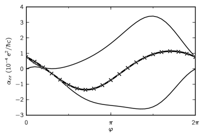
Figure 4: Comparison between $\alpha_{zz}$ calculated treating the two lowest bands as occupied (crosses) and the sum $\alpha_{zz}^{(1)}+\alpha_{zz}^{(2)}$ (thick solid line), where $\alpha_{zz}^{(n)}$ (thin solid lines) correspond to treating only the lowest band ($n=1$, upper line) or the second-lowest band ($n=2$, lower line) as occupied. Model parameters are the same as for figure 1 except that the second lowest on-site energy in table 1 is raised from $-$6.0 to $-$5.0 in order to keep the two lowest bands well-separated.

It could have been anticipated from the outset that the Chern-Simons term (6ahaoaua) could not be the entire expression for the OMP, based on the following argument [26]. Consider an insulator with $N>1$ valence bands, all of which are isolated from one another. By looking at $\alpha_{da}$ as $\partial P_{d}/\partial B_{a}$ one can argue that, since each band carries a certain amount of polarization ${\bi P}^{(n)}$, the total OMP should satisfy the relation

$$\alpha=\sum_{n}^{N}\,\alpha^{(n)},$$ (6ahaoauay)

where $\alpha^{(n)}$ is the OMP one would obtain by filling band $n$ while keeping all other bands empty. We shall refer to this property as the “band-sum-consistency” of the OMP. It only holds exactly for models without charge self-consistency (see the analytic proof in C), but that suffices for the purpose of the argument. We note that the Chern-Simons contribution (6ahaoaua) alone is not band-sum-consistent, because the second term therein vanishes for a single occupied band. Hence an additional contribution, also band-sum-inconsistent, must necessarily exist. Indeed, both $\widetilde{\alpha}^{\rm LC}$ and $\widetilde{\alpha}^{\rm IC}$ are band-sum-inconsistent, in such a way that the total OMP satisfies (6ahaoauay). This is illustrated in figure 4 for our tight-binding model.

4 Summary and outlook

In summary, we have developed a theoretical framework for calculating the frozen-ion orbital-magnetization response (OMP) to a static electric field. This development fills an important gap in the microscopic theory of the magnetoelectric effect, paving the way to first-principles calculations of the full response. While the OMP is often assumed to be small compared to the lattice-mediated and spin-magnetization parts of the ME response, there is no a priori reason why it should always be so. In fact, in strong $Z_{2}$ topological insulators it is the only contribution that survives, and the predicted value is large compared to that of prototypical magnetoelectrics. Although the measurement of the $\theta=\pi$ ME effect in topological insulators is challenging, as time-reversal symmetry must be broken to gap the surfaces [6, 7, 23], there may be other related materials where those symmetries are broken already in the bulk. The present formalism should be helpful in the ongoing computational search for such materials with a large and robust OMP.

A key result of this work is a $k$-space expression for the orbital magnetization of a periodic insulator under a finite electric field ${\boldsymbol{\mathcal{E}}}$ (equations (6a)–(6d), or equivalently, (6aha)–(6ahd)). In addition to the terms (6ahb)–(6ahc) already present at zero field [13], in three dimensions the field-dependent magnetization comprises an additional purely isotropic ‘Chern-Simons’ term, given by (6ahd). This new term depends explicitly on ${\boldsymbol{\mathcal{E}}}$ and only implicitly on $H^{0}_{\bi k}$, while the converse is true for the other terms. Moreover, it is a multivalued quantity, with a quantum of arbitrariness ${\bi M}_{0}={\boldsymbol{\mathcal{E}}}e^{2}/hc$ along ${\boldsymbol{\mathcal{E}}}$. Thus, the analogy with the Berry-phase theory of electric polarization [10, 20], where a similar quantum arises, becomes even more profound at finite electric field.

The Chern-Simons term ${\bi M}^{\rm CS}$ is responsible for the geometric part of the OMP response discussed in [6, 7] in connection with topological insulators. We have clarified that in materials with broken time-reversal and inversion symmetries in the bulk the CSOMP does not generally constitute the full response, as the remaining orbital magnetization terms, ${\widetilde{\bi M}}^{\rm LC}$ and $\widetilde{{\bi M}}^{\rm IC}$, can also depend linearly on ${\boldsymbol{\mathcal{E}}}$. Their contribution to the OMP, given by (6ahaoau)–(6ahaoau), is twofold: (i) to modify the isotropic coupling strength $\theta$; and (ii) to introduce an anisotropic component of the response.

Another noteworthy result is equation (6ahaoas) for the Chern-Simons OMP of finite systems. One appealing feature of this expression is that it allows one to calculate the CSOMP without the need to choose a particular gauge. Instead, its $k$-space counterpart, equation (6ahaoaua), requires for its numerical evaluation a smoothly varying gauge for the Bloch states across the Brillouin zone. Equation (6ahaoas) is also the more general of the two, as it can be applied to noncrystalline or otherwise disordered systems.

We conclude by enumerating a few questions that are raised by the present work. Do the individual gauge-invariant OMP terms identified here in a one-electron picture remain meaningful for interacting systems, and can they be separated experimentally? (This appears to be the case for ${\widetilde{\bi M}}^{\rm LC}$ and $\widetilde{{\bi M}}^{\rm IC}$ at ${\boldsymbol{\mathcal{E}}}=0$ [35].) How does the expression (6ahaoaua)–(6ahaoau) for the linear OMP response change when the reference state is under a finite electric field ${\boldsymbol{\mathcal{E}}}$? Finally, we note that equation (6ahaoc) for the CSOMP of finite systems has a striking resemblance to a formula given by Kitaev [39] for the 2-D Chern invariant characterizing the integer quantum Hall effect. Can this connection be made more precise, in view of the fact that the quantum of indeterminacy in $\theta^{\rm CS}$ is associated with the possibility of changing the Chern invariant of the surface layers? These questions are left for future studies.

Appendix A Tight-binding model and technical details

Tight-binding model

We have chosen for our tests a model of an ordinary (that is, non-topological) insulator. The prerequisites were the following. It should break both time-reversal and inversion symmetries, as the OMP tensor otherwise vanishes identically. It should be three-dimensional, as the geometric part of the response vanishes otherwise. Its symmetry should be sufficiently low to render all nine components of the OMP tensor nonzero. Finally, it should have multiple valence bands, for generality.

We opted for a spinless model on a cubic lattice. It can be obtained starting with a one-site simple cubic model, doubling the cell in each direction, and assigning random on-site energies $E_{{\bi i}}$ and complex first-neighbour hoppings $t_{{\bi j}\to{\bi i}}=t\rme^{\rmi\phi_{{\bi j}\to{\bi i}}}$ of fixed magnitude $t=1$. The Hamiltonian reads

$$\mathcal{H}^{0}=\sum_{{\bi i}}\,E_{{\bi i}}c^{\dagger}_{{\bi i}}c^{\phantom{\dagger}}_{{\bi i}}+\sum_{\langle{\bi i}{\bi j}\rangle}\,\rme^{\rmi\phi_{{\bi j}\to{\bi i}}}c^{\dagger}_{{\bi i}}c^{\phantom{\dagger}}_{{\bi j}},$$ (6ahaoauaz)

where ${\bi i}=(x,y,z)$ labels the sites and $\langle{\bi i\bi j}\rangle$ denotes pairs of nearest-neighbour sites. The values of $E_{{\bi i}}$ on two of the eight sites were adjusted to ensure a finite gap everywhere in the Brillouin zone between the two lowest bands (chosen as the valence bands) and the remaining six. We also made sure that nonzero phases $\phi_{{\bi j}\to{\bi i}}$ were not restricted to two-dimensional square-lattice planes, otherwise those are mirror symmetry planes, whose existence is sufficient to make the diagonal elements of the OMP tensor vanish. In our calculations all the model parameters were kept fixed except for one phase, which was scanned over the range $[0,2\pi]$, and the results are plotted as a function of this phase $\varphi$. For reference, the on-site energies and the phases of the hopping amplitudes are listed in table 1. The energy bands are shown in figure 5 for $\varphi=0$.

In order to couple the system to the electric field and to be able to define its orbital magnetization, the position operator ${\bi r}$ must be specified along with $\mathcal{H}^{0}$. We have chosen the simplest representation where ${\bi r}$ is diagonal in the tight-binding basis.

Table 1: The parameters of the tight-binding model. Columns I–III give the site coordinates ${\bi i}=(x,y,z)$, in units of the lattice constant $a=1$ of the $2\times 2\times 2$ primitive cubic cell. Column IV contains the on-site energies $E_{{\bi i}}$, and the last three columns contain the phases of the complex nearest-neighbour hopping amplitudes along bonds in the negative $\hat{\bi x}$, $\hat{\bi y}$, and $\hat{\bi z}$ directions.

• $x$	$y$	$z$	$E_{{\bi i}}$	$\phi_{\mbox{\scriptsize$({\bi i}+\hat{\bi x}/2)\to{\bi i}$}}$	$\phi_{\mbox{\scriptsize$({\bi i}+\hat{\bi y}/2)\to{\bi i}$}}$	$\phi_{\mbox{\scriptsize$({\bi i}+\hat{\bi z}/2)\to{\bi i}$}}$
  0.0	0.0	0.0	$-$6.5	$\varphi\in[0,2\pi]$	0.5$\pi$	1.7$\pi$
  0.5	0.0	0.0	0.9	1.3$\pi$	0.2$\pi$	0.5$\pi$
  0.5	0.5	0.0	1.4	0.8$\pi$	1.4$\pi$	0.6$\pi$
  0.0	0.5	0.0	1.2	0.3$\pi$	1.9$\pi$	1.0$\pi$
  0.0	0.0	0.5	$-$6.0	1.4$\pi$	0.8$\pi$	0.3$\pi$
  0.5	0.0	0.5	1.5	0.6$\pi$	1.7$\pi$	0.7$\pi$
  0.5	0.5	0.5	0.8	0.8$\pi$	0.6$\pi$	1.2$\pi$
  0.0	0.5	0.5	1.2	1.9$\pi$	0.3$\pi$	1.4$\pi$

• In figure 4 the value $-$5.0 was used instead.

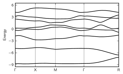
Figure 5: Band structure of the cubic-lattice tight-binding model given by (6ahaoauaz), for the choice of parameters in table 1 and $\varphi=0$.

Technical details

The calculations employing periodic boundary conditions were carried out on an $80\times 80\times 80$ $k$-point mesh, and the $k$-space implementation of finite electric fields was done using the method discussed in section V of [30]. The open boundary condition calculations used cubic samples containing $L\times L\times L$ eight-site unit cells, that is, $2L+1$ sites along each edge. For large $L$, we expect the magnetization to scale as

$${\bi M}(L)={\bi M}+\frac{{\bi a}}{L}+\frac{{\bi b}}{L^{2}}+\frac{{\bi c}}{L^{3}},$$ (6ahaoauba)

where ${\bi a}$, ${\bi b}$, and ${\bi c}$ account for face, edge, and corner corrections, respectively [13]. Calculations of ${\bi M}(L)$ under small fields were done using $L=4,5,6,7$, and then fitted to (6ahaoauba) in order to extract the value ${\bi M}$ of the magnetization in the $L\to\infty$ limit. The differences between OMP values calculated in various ways as shown in figures 1 and 2 were of the order of $10^{-7}$ $e^{2}/\hbar c$ or less.

Before evaluating the $k$-space expressions for ${\bi M}({\boldsymbol{\mathcal{E}}})$ [(6a)–(6d) and (6ahb)–(6ahd)] and $\alpha$ [(6ahaoaua)–(6ahaoau)] on a grid, they need to be properly discretized. The presence of the gauge-dependent Berry connection in (6d) demands the use of a “smooth gauge” for its evaluation, where the valence Bloch states given by (6r) are smoothly varying functions of ${\bi k}$. This is achieved by projecting a set of trial orbitals onto the set of occupied Bloch eigenstates according to the prescription in equations (62–64) of [31]. (For the tight-binding model discussed below, when treating the two lowest bands as occupied, the two trial orbitals are chosen as delta functions located at the two sites with lowest on-site energy.) If needed, this one-shot projection procedure can be improved upon by finding an optimally smooth gauge using methods based on minimizing the real-space spread of the WFs [31], but we found our results to change negligibly when performing this extra step. In a smooth gauge the needed $k$-derivatives of the Bloch states and of the Berry connection matrix are then evaluated by straightforward numerical differentiation. Note that (6b) and (6c) should be evaluated in the same smooth gauge as (6d), as these three equations are not separately gauge-invariant. A smooth gauge must also be used for (6ahd) and (6ahaoaua), because, as discussed in section 2.3.1, the Chern-Simons 3-form is locally gauge-dependent.

The same strategy can be used to discretize (6ahb) and (6ahc). However, since the $k$-derivatives appearing in those equations are covariant, the discretized form of the covariant derivative (6s) given in [30, 13] may be used instead, circumventing the need to work in a smooth gauge. We have implemented both approaches, finding excellent agreement between them.

Finally we come to equations (6ahaoau) and (6ahaoau). In addition to the $k$-derivative of the valence Bloch states, we need their (covariant) field-derivative (6ahaoauav), as well as the $k$-derivative of $H^{0}_{\bi k}$. The latter quantity is easily calculated within the tight-binding method, and for the former we used the linear-response expression (6ahaoauax). Note that this requires choosing the unperturbed states to be in the Hamiltonian gauge. This choice precludes calculating the $k$-derivative on the right-hand-side of (6ahaoauax) by straightforward finite differences, which can only be done in a smooth gauge. But because $\langle u^{0}_{m{\bi k}}|\partial_{d}u^{0}_{n{\bi k}}\rangle$ equals $\langle u^{0}_{m{\bi k}}|\widetilde{\partial}_{d}u^{0}_{n{\bi k}}\rangle$ for $m>N$, the discretized covariant derivative approach may be used instead. Alternatively, one can evaluate the ordinary $k$-derivative by summation over states as

$$|\partial_{d}u_{n{\bi k}}^{0}\rangle=\sum_{m\not=n}\,|u_{m{\bi k}}^{0}\rangle\frac{\langle u_{m{\bi k}}^{0}|(\partial_{d}H^{0}_{\bi k})|u_{n{\bi k}}^{0}\rangle}{E_{n{\bi k}}^{0}-E_{m{\bi k}}^{0}}.$$ (6ahaoaubb)

We note that this formula may not be used to calculate the geometric term (6ahaoaua), because it induces locally a parallel transport gauge ($A_{nn}^{0}=0$), which cannot be enforced globally since the Brillouin zone is a closed space.

Appendix B Derivation of equations (6ahaoau) and (6ahaoau)

For notational simplicity we drop the crystal momentum index ${\bi k}$. So, for example, $|u_{n{\bi k}}\rangle$ shall be denoted by $|u_{n}\rangle$. In order to calculate the OMP terms

$$\widetilde{\alpha}^{\rm LC}_{da}=\left.\partial_{D}\widetilde{M}_{a}^{({\rm LC})}\right|_{{\boldsymbol{\mathcal{E}}}=0}$$ (6ahaoaubc)

and

$$\widetilde{\alpha}^{\rm IC}_{da}=\left.\partial_{D}\widetilde{M}_{a}^{({\rm IC})}\right|_{{\boldsymbol{\mathcal{E}}}=0}$$ (6ahaoaubd)

starting from (6ae) and (6af), we shall first examine the field- and $k$-derivatives of certain basic quantities.

We begin by noting that the field-derivative $\partial_{D}P=-\partial_{D}Q$ of the projection operator (6t) can be written as

$$\partial_{D}P=\sum_{n}^{N}\left(|\widetilde{\partial}_{D}u_{n}\rangle\langle u_{n}|+|u_{n}\rangle\langle\widetilde{\partial}_{D}u_{n}|\right)\equiv\widetilde{\partial}_{D}P,$$ (6ahaoaube)

in terms of the covariant field-derivative (6ahaoauav) (a similar expression holds for the $k$-derivative). This follows from a relation analogous to (6u):

$$|\partial_{D}u_{n}\rangle=|\widetilde{\partial}_{D}u_{n}\rangle-\rmi\sum_{l}^{N}A_{ln,D}|u_{l}\rangle,$$ (6ahaoaubf)

where

$$A_{ln,D}=\rmi\langle u_{l}|\partial_{D}u_{n}\rangle=A_{nl,D}^{*}$$ (6ahaoaubg)

is the Berry connection matrix along the parametric direction $\mathcal{E}_{d}$. With the help of (6ahaoaube) the field-derivative of (6v) becomes

$$\partial_{D}F_{nm,bc}=\langle\partial^{2}_{Db}u_{n}|Q|\partial_{c}u_{m}\rangle+\langle\partial_{b}u_{n}|Q|\partial^{2}_{Dc}u_{m}\rangle+\rmi(F_{bD}A_{c})_{nm}-\rmi(A_{b}F_{Dc})_{nm},$$

where $F_{bD}$ is obtained from $F_{bd}$ by replacing $\partial_{d}$ with $\partial_{D}$. We shall also need the field- and $k$-derivatives of the matrix $H^{0}_{nm}$ defined by (6h):

$$\left.\partial_{D}(H_{nm}^{0})\right|_{{\boldsymbol{\mathcal{E}}}=0}=\rmi\left[A_{D}^{0},H^{0}\right]_{nm}+\left.(\partial_{D}H^{0}_{\mathrm{op}})_{nm}\right|_{{\boldsymbol{\mathcal{E}}}=0}$$ (6ahaoaubh)

$$\left.\partial_{c}(H_{nm}^{0})\right|_{{\boldsymbol{\mathcal{E}}}=0}=\rmi\left[A_{c}^{0},H^{0}\right]_{nm}+\left.(\partial_{c}H^{0}_{\mathrm{op}})_{nm}\right|_{{\boldsymbol{\mathcal{E}}}=0},$$ (6ahaoaubi)

where we introduced the notation $(\partial_{D,c}H^{0}_{\mathrm{op}})_{nm}\equiv\langle u_{n}|\partial_{D,c}H^{0}|u_{m}\rangle$, where ‘op’ indicates that the derivative is taken on the operator itself, not its matrix representation. These two relations follow directly from (6ahaoaubf) and (6u). We will also make use of identities such as

$$\mathrm{Re\,tr}\left[XF_{bc}\right]=\mathrm{Re\,tr}\left[X^{\dagger}F_{cb}\right].$$ (6ahaoaubj)

In particular, if $X$ and $Y$ are Hermitian,

$$\mathrm{Re\,tr}\left[XYF_{bc}\right]=\mathrm{Re\,tr}\left[YXF_{cb}\right].$$ (6ahaoaubk)

We are now ready to evaluate (6ahaoaubd):

$$\widetilde{\alpha}^{\rm IC}_{da}=-\gamma\epsilon_{abc}\int[\rmd k]\mathrm{Im\,}\tr\bigl{[}F_{bc}\partial_{D}H^{0}+\left.H^{0}\partial_{D}F_{bc}\bigr{]}\right|_{{\boldsymbol{\mathcal{E}}}=0}.$$ (6ahaoaubl)

Inserting (B) and (6ahaoaubh) on the right-hand side generates a number of terms. Some can be combined upon interchanging dummy indices $b\leftrightarrow c$ and invoking (6ahaoaubk), leading to

$$\widetilde{\alpha}^{\rm IC}_{da}=-\gamma\epsilon_{abc}\int[\rmd k]\Big{(}2\mathrm{Re\,tr}\left[A_{D}H^{0}F_{bc}+H^{0}F_{bD}A_{c}\right]+\mathrm{Im\,}\tr\left[F_{bc}\partial_{D}H^{0}_{\rm op}\right]$$

$$\;\;\;\;\;\;\;\;+2\mathrm{Im}\sum_{mn}^{N}H^{0}_{mn}\langle\partial^{2}_{Db}u_{n}|Q|\partial_{c}u_{m}\rangle\Big{)}\Big{|}_{{\boldsymbol{\mathcal{E}}}=0}.$$ (6ahaoaubm)

Integrating the last term by parts in $k_{b}$ and using (6ahaoaube) and (6ahaoaubi) again produces a number of terms, most of which cancel out. The end result reads

$$\widetilde{\alpha}^{\rm IC}_{da}=\gamma\epsilon_{abc}\int[\rmd k]\,\mathrm{Im\,}\tr\left.\left[2F_{bD}\partial_{c}H^{0}_{\mathrm{op}}-F_{bc}\partial_{D}H^{0}_{\rm op}\right]\right|_{{\boldsymbol{\mathcal{E}}}=0}.$$ (6ahaoaubn)

Similarly, (6ahaoaubc) can be evaluated by repeatedly using (6ahaoaube) and integrating by parts the terms with mixed field- and $k$-derivatives, yielding

$$\widetilde{\alpha}^{\rm LC}_{da}=\gamma\epsilon_{abc}\int[\rmd k]\,\mathrm{Im\,}\tr\left.\left[2(\partial_{c}H^{0})_{bD}-(\partial_{D}H^{0})_{bc}\right]\right|_{{\boldsymbol{\mathcal{E}}}=0},$$ (6ahaoaubo)

where $(\partial_{c}H^{0})_{bD}$ and $(\partial_{D}H^{0})_{bc}$ are defined in analogy with (6z), e.g.,

$$(\partial_{c}H^{0})_{nm{\bi k},bD}=\langle\widetilde{\partial}_{b}u_{n{\bi k}}|(\partial_{c}H^{0}_{\bi k})|\widetilde{\partial}_{D}u_{m{\bi k}}\rangle.$$ (6ahaoaubp)

Equations (6ahaoaubo) and (6ahaoaubn) are respectively equivalent to (6ahaoau) and (6ahaoau) in the main text. The gauge invariance of these equations follows from the fact that they are written as traces over gauge-covariant objects. (We also note that the covariant derivative transforms according to (6r) regardless of the parameter with respect to which the differentiation is carried out.)

Appendix C Band-sum consistency of the OMP

Here we show analytically that the OMP tensor $\alpha$ satisfies the band-additivity relation (6ahaoauay) in models without charge self-consistency. In order to isolate the contribution $\alpha^{(n)}$ coming from valence band $n$ (assumed to be well-separated in energy from all other bands), we choose the Hamiltonian matrix to be diagonal at zero field, i.e., $H^{0}_{mn{\bi k}}({\boldsymbol{\mathcal{E}}}=0)=E_{n{\bi k}}^{0}\delta_{mn}$. If in addition we use a parallel-transport gauge for the linear electric field perturbation [33] (this is achieved by setting to zero the matrix $A_{D}$ defined in (6ahaoaubg)) we find, using (6ahaoaubh), $\partial_{D}H^{0}_{mn{\bi k}}|_{{\boldsymbol{\mathcal{E}}}=0}=0$. With the help of these two relations, the field-derivative $\partial_{D}M_{a}|_{{\boldsymbol{\mathcal{E}}}=0}$ of (6a) is easily taken. From the first two terms therein we obtain (dropping the index ${\bi k}$)

$$\left.2\gamma\epsilon_{abc}\int[\rmd k]\,\sum_{n}^{N}\,\mathrm{Im}\langle\partial_{b}u_{n}|\partial_{c}(H^{0}+E_{n})|\partial_{D}u_{n}\rangle\right|_{{\boldsymbol{\mathcal{E}}}=0}.$$ (6ahaoaubq)

In the parallel-transport gauge $|\partial_{D}u_{n}\rangle$ is given by (6ahaoauax), and combining the resulting expression with the field-derivative of the third term in (6a) yields

$$\alpha_{da}=2e\gamma\epsilon_{abc}\int[\rmd k]\,\sum_{n}^{N}\,\mathrm{Re}\langle\partial_{b}u_{n}^{0}|\partial_{c}(H^{0}+E_{n}^{0})\left(\sum_{l>N}\,\frac{|u_{l}^{0}\rangle\langle u_{l}^{0}|}{E_{n}^{0}-E_{l}^{0}}\right)|\partial_{d}u_{n}^{0}\rangle$$

$$-e\gamma\epsilon_{abc}\,\int[\rmd k]\,\sum_{mn}^{N}\,\mathrm{Re}\left(\langle u_{m}^{0}|\partial_{d}u_{n}^{0}\rangle\langle\partial_{b}u_{n}^{0}|\partial_{c}u_{m}^{0}\rangle\right).$$ (6ahaoaubr)

To find $\alpha_{da}^{(n)}$ we replace $\sum_{l>N}$ with $\sum_{l\not=n}$ and reduce sums $\sum_{mn}^{N}$ and $\sum_{n}^{N}$ to single terms. Inserting these expressions into (6ahaoauay) and splitting $\sum_{l\not=n}$ into $\sum_{l>N}$ and $\sum_{l\not=n}^{N}$, some terms cancel and others can be combined, leading to

$$\epsilon_{abc}\int[\rmd k]\,\sum_{n}^{N}\,\sum_{m\not=n}^{N}\,\mathrm{Re}\Biggl{[}\langle u_{m}^{0}|\partial_{d}u_{n}^{0}\rangle$$

$$\times\left(\frac{\langle\partial_{b}u_{n}^{0}|\partial_{c}(H^{0}+E_{n}^{0})|u_{m}^{0}\rangle}{E_{n}^{0}-E_{m}^{0}}+\frac{1}{2}\langle\partial_{b}u_{n}^{0}|\partial_{c}u_{m}^{0}\rangle\right)\Biggr{]}=0.$$ (6ahaoaubs)

The LHS is proportional to the difference between $\alpha_{da}$ and $\sum_{n}^{N}\,\alpha_{da}^{(n)}$, and vanishes as a result of an exact cancellation between the terms $(n,m)$ and $(m,n)$ in the double sum. The integrand of the $(n,m)$ term is

$$\epsilon_{abc}\mathrm{Re}\left[\langle u_{m}^{0}|\partial_{d}u_{n}^{0}\rangle\left(\frac{\langle\partial_{b}u_{n}^{0}|\partial_{c}(H^{0}+E_{n}^{0})|u_{m}^{0}\rangle}{E_{n}^{0}-E_{m}^{0}}+\frac{1}{2}\langle\partial_{b}u_{n}^{0}|\partial_{c}u_{m}^{0}\rangle\right)\right],$$ (6ahaoaubt)

and after some manipulations the integrand of the $(m,n)$ term becomes

$$\epsilon_{abc}\mathrm{Re}\left[\langle u_{m}^{0}|\partial_{d}u_{n}^{0}\rangle\left(\frac{\langle u_{n}^{0}|\partial_{c}(H^{0}+E_{m}^{0})|\partial_{b}u_{m}^{0}\rangle}{E_{n}^{0}-E_{m}^{0}}+\frac{1}{2}\langle\partial_{b}u_{n}^{0}|\partial_{c}u_{m}^{0}\rangle\right)\right].$$ (6ahaoaubu)

The final step is to use the identity

$$\frac{\langle\partial_{b}u_{n}^{0}|\partial_{c}(H^{0}+E_{n}^{0})|u_{m}^{0}\rangle}{E_{n}^{0}-E_{m}^{0}}=\frac{\langle\partial_{b}u_{n}^{0}|E_{m}^{0}-H^{0}|\partial_{c}u_{m}^{0}\rangle}{E_{n}^{0}-E_{m}^{0}}-\partial_{c}(E_{n}^{0}+E_{m}^{0})\frac{\langle u_{n}^{0}|\partial_{b}u_{m}^{0}\rangle}{E_{n}^{0}-E_{m}^{0}}.$$ (6ahaoaubv)

(This identity follows from the relation

$$(H^{0}-E_{m}^{0})|\partial_{c}u_{m}^{0}\rangle=-(\partial_{c}H^{0}-\partial_{c}E_{m}^{0})|u_{m}^{0}\rangle,$$ (6ahaoaubw)

which in turn can be obtained by expanding $H^{0}|u_{m}^{0}\rangle=E_{m}^{0}|u_{m}^{0}\rangle$ to first order in the change in wavevector ${\bi k}$.) The quantity (6ahaoaubt)+(6ahaoaubu) then becomes

$$\epsilon_{abc}\mathrm{Re}\left[\langle u_{m}^{0}|\partial_{d}u_{n}^{0}\rangle\left(\frac{\langle\partial_{b}u_{n}^{0}|E_{m}^{0}-H^{0}|\partial_{c}u_{m}^{0}\rangle}{E_{n}^{0}-E_{m}^{0}}+\frac{\langle\partial_{c}u_{n}^{0}|E_{n}^{0}-H^{0}|\partial_{b}u_{m}^{0}\rangle}{E_{n}^{0}-E_{m}^{0}}+\langle\partial_{b}u_{n}^{0}|\partial_{c}u_{m}^{0}\rangle\right)\right].$$ (6ahaoaubx)

Interchanging $b\leftrightarrow c$ in the second term and combining with the first yields minus the third term, which concludes the proof.

References

References

- [1] O’Dell T 1970 The Electrodynamics of Magneto-Electric Media (Amsterdam: North-Holland)
- [2] Fiebig M 2005 J. Phys. D 38 R123
- [3] Íñiguez J 2008 Phys. Rev. Lett. 101 117201
- [4] Wojdel J and Íñiguez J 2009 Phys. Rev. Lett. 103 267205
- [5] Delaney K T and Spaldin N A 2009 arXiv:0912.1335
- [6] Qi X, Hughes T L and Zhang S C 2008 Phys. Rev. B 78 195424
- [7] Essin A M, Moore J E and Vanderbilt D 2009 Phys. Rev. Lett. 102 146805
- [8] Raab R E and De Lange O L 2005 Multipole Theory in Electromagnetism (Oxford: Clarendon Press)
- [9] Barron L D 2004 Molecular Light Scattering and Optical Activity (Cambridge: Cambridge University Press)
- [10] King-Smith R D and Vanderbilt D 1993 Phys. Rev. B 47 1651
- [11] Xiao D, Shi J and Niu Q 2005 Phys. Rev. Lett. 95 137204
- [12] Thonhauser T, Ceresoli D, Vanderbilt D and Resta R 2005 Phys. Rev. Lett. 95 137205
- [13] Ceresoli D, Thonhauser T, Vanderbilt D and Resta R 2006 Phys. Rev. B 74 024408
- [14] Shi J, Vignale G, Xiao D and Niu Q 2007 Phys. Rev. Lett. 99 197202
- [15] Wilczek F 1987 Phys. Rev. Lett. 58 1799
- [16] Raab R E and Sihvola A H 1997 J. Phys. A: Math. Gen. 30 1335
- [17] Hehl F W, Obukhov Y N, Rivera J P and Schmid H 2008 Phys. Rev. A 77 022106
- [18] Obukhov Y N and Hehl F W 2005 Phys. Lett. A 341 357
- [19] Widom A, Friedman M H and Srivastava Y 1986 J. Phys. A: Math. Gen. 19 L175
- [20] Resta R and Vanderbilt D 2007 Theory of polarization: A modern approach Physics of Ferroelectrics: A Modern Perspective ed Rabe K M, Ahn C H and Triscone J M (Berlin: Springer-Verlag) pp 31–68
- [21] Chern S S and Simons J 1974 Ann. Math. 99 48
- [22] Qi X L and Zhang S C 2010 Physics Today January 33
- [23] Hasan M Z and Kane C L 2010 arXiv:1002.3895
- [24] Moore J E 2010 Nature 464 194
- [25] Wiegelmann H, Jansen A G M, Wyder P, Rivera J P and Schmid H 1994 Ferroelectrics 162 141
- [26] Essin A, Turner A, Moore J and Vanderbilt D arXiv:1002.0290
- [27] Thonhauser T and Vanderbilt D 2006 Phys. Rev. B 74 235111
- [28] Haldane F D M 1988 Phys. Rev. Lett. 61 2015
- [29] Souza I, Íñiguez J and Vanderbilt D 2002 Phys. Rev. Lett. 89 117602
- [30] Souza I, Íñiguez J and Vanderbilt D 2004 Phys. Rev. B 69 085106
- [31] Marzari N and Vanderbilt D 1997 Phys. Rev. B 56 12847
- [32] Blount E I 1962 Solid State Physics vol 13 ed Seitz F and Turnbull D (New York: Academic)
- [33] Nunes R W and Gonze X 2001 Phys. Rev. B 63 155107
- [34] Nakahara M 1998 Geometry, Topology and Physics (Bristol: Institute of Physics)
- [35] Souza I and Vanderbilt D 2008 Phys. Rev. B 77 054438
- [36] Umari P and Pasquarello A 2002 Phys. Rev. Lett. 89 157602
- [37] Baroni S, de Gironcoli S, Corso A D and Giannozzi P 2001 Rev. Mod. Phys. 73 515
- [38] Essin A, Moore J E and Vanderbilt D 2009 Phys. Rev. Lett. 103 259902
- [39] Kitaev A 2006 Ann. Phys. (NY) 321 2