VLT-MAD observations of the core of 30 Doradus

Abstract

We present $H$- and $K_{\rm s}$-band imaging of three fields at the centre of 30 Doradus in the Large Magellanic Cloud, obtained as part of the Science Demonstration programme with the Multi-conjugate Adaptive optics Demonstrator (MAD) at the Very Large Telescope. Strehl ratios of 15-30% were achieved in the $K_{\rm s}$-band, yielding near-infrared images of this dense and complex region at unprecedented angular resolution at these wavelengths.

The MAD data are used to construct a near-infrared luminosity profile for R136, the cluster at the core of 30 Dor. Using cluster profiles of the form used by Elson et al., we find the surface brightness can be fit by a relatively shallow power-law function ($\gamma$ $\sim$ 1.5-1.7) over the full extent of the MAD data, which extends to a radius of $\sim$40^′′ ($\sim$10 pc). We do not see compelling evidence for a break in the luminosity profile as seen in optical data in the literature, arguing that cluster asymmetries are the dominant source, although extinction effects and stars from nearby triggered star-formation likely also contribute. These results highlight the need to consider cluster asymmetries and multiple spatial components in interpretation of the luminosity profiles of distant unresolved clusters.

We also investigate seven candidate young stellar objects reported by Gruendl & Chu from Spitzer observations, six of which have apparent counterparts in the MAD images. The most interesting of these (GC09: 053839.24 $-$690552.3) appears related to a striking bow-shock–like feature, orientated away from both R136 and the Wolf-Rayet star Brey 75, at distances of 19$\aas@@fstack{\prime\prime}$5 and 8^′′ (4.7 and 1.9 pc in projection), respectively.

1 Introduction

30 Doradus in the Large Magellanic Cloud (LMC) is the largest star-forming region in the Local Group. As an archetypal, small-scale ‘starburst’, 30 Dor provides us with an excellent laboratory in which to study star formation and stellar evolution, while also giving us potential insights into the nature of distant super-star-clusters for which we only have integrated properties. Extensive ground-based optical imaging and spectroscopy has been used to study the initial mass function (IMF), reddening, star-formation history, stellar content and kinematics in 30 Dor (e.g. Melnick, 1985; Parker, 1993; Parker & Garmany, 1993; Walborn & Blades, 1997; Selman, 1998; Bosch et al., 2001). Meanwhile, near-IR observations with the Hubble Space Telescope (HST) have provided evidence of triggered star-formation, showing the region to be a two-stage starburst (Walborn et al., 1999, 2002).

At the centre of 30 Dor is the dense star cluster R136, with stellar ages for the most massive stars in the range of 1-2 Myr (Massey & Hunter, 1998) and a total stellar mass in the range of $\sim$0.35-1$\times 10^{5}$ M_⊙ (e.g. Mackey & Gilmore, 2003; Noyola & Gebhardt, 2007; Andersen et al., 2009), depending on the low-mass form of the mass function, putting it on a par with some of the clusters found in starburst and interacting galaxies such as M51, M82 and the Antennae. However, the core of R136 is too dense for traditional (seeing-limited) ground-based techniques.

Only with the arrival of HST was R136 resolved in optical and UV images (Campbell et al., 1992; de Marchi et al., 1993; Hunter et al., 1995; Hunter et al., 1997; Sirianni et al., 2000), with follow-up spectroscopy revealing a hitherto unprecedented concentration of the earliest O-type stars (Massey & Hunter, 1998). Star counts from the optical HST images revealed that the luminosity profile of R136 appears to be best described by two components, with a break at 10^′′ (Mackey & Gilmore, 2003). New results from F160W imaging (equivalent to $H$-band) with the HST Near Infrared Camera and Multi-Object Spectrometer (NICMOS) fit the profile with a single component (Andersen et al., 2009), but only in the inner 2 pc (8$\aas@@fstack{\prime\prime}$25). Whether the second component seen in the optical data is a manifestation of the ‘excess light’ predicted to originate from rapid gas removal in the early stages of cluster evolution (Bastian & Goodwin, 2006) remains an open question as there is significant and variable extinction across the cluster.

As part of the technology development plan towards the European Extremely Large Telescope (E-ELT), the Multi-conjugate Adaptive optics Demonstrator (MAD, Marchetti et al., 2007) was developed as a visiting instrument for the Very Large Telescope (VLT). The offer of Science Demonstration (SD) observations with MAD presented the perfect opportunity to obtain imaging of R136 at unprecedented angular resolution at near-IR wavelengths. In particular, MAD has the power to penetrate the gas and dust more successfully than in the optical HST images, at comparable angular resolution, to provide empirical constraints on the outer component on the luminosity profile. Determining if R136 is an expanding group or a dynamically-stable star cluster would serve as an important ingredient in the debate on the importance of ‘infant mortality’ of young clusters (e.g. Lada & Lada, 2003; Bastian et al., 2005; Fall et al., 2005; Goodwin & Bastian, 2006; Baumgardt & Kroupa, 2007; Bastian et al., 2008).

Here we present the MAD SD observations, which deliver a cleaner point spread function (PSF) than NICMOS, at finer angular resolution, and over a larger total field. The instrumental performance of MAD is discussed in Section 2, with the astrometric and photometric calibration of the data detailed in Sections 3 and 4, respectively. Following discussion of seven of the candidate young stellar objects (YSOs) reported by Gruendl & Chu (2009, hereafter GC09) that lie within the MAD fields (Section 5), we then investigate the radial luminosity profile of R136 via a combination of star counts and integrated-light measurements (Section 6), discussing its implications in the context of cluster formation and observations of distant unresolved clusters.

2 Observations & Data Reduction

MAD employs three Shack-Hartmann wavefront sensors to observe three natural guide stars (NGS) across a 2^′ circular field, thereby allowing tomography of the atmospheric turbulence. The turbulence is then corrected using two deformable mirrors (operating at $\sim$400 Hz), one conjugated to the ground-layer (i.e. 0 km), the second conjugated to 8.5 km above the telescope.

The high resolution, near-IR camera used with MAD is the CAmera for Multi Conjugate Adaptive Optics (CAMCAO, Amorim et al., 2006), which operates over the J, $H$, and $K_{\rm s}$ bands, with critical (2 pixel) sampling of the diffraction-limited PSF at 2.2$\mu$m. The detector is a 2k$\times$2k Hawaii-2 HgCdTe array, with a pixel scale of 0$\aas@@fstack{\prime\prime}$028/pixel, giving a field-of-view of 57^′′x57^′′. A useful feature is that the camera can be moved within the 2^′ field without requiring positional offsets of the telescope, meaning that the adaptive optics (AO) loop can remain closed.

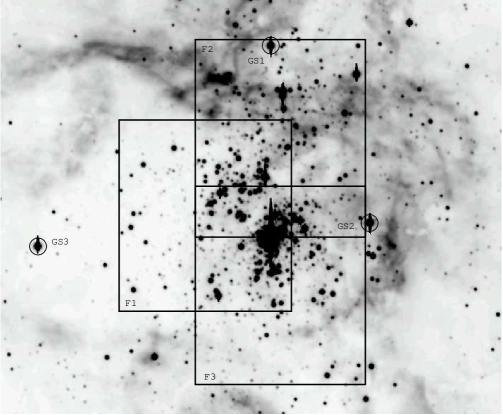
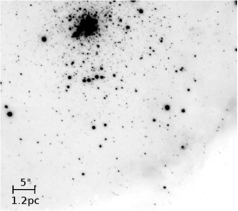
Figure 1: $V$-band image of the central part of 30 Dor (approx 3$\aas@@fstack{\prime}$0 by 2$\aas@@fstack{\prime}$5) from the Wide-Field Imager (WFI) on the ESO/Max Planck Gesellschaft 2.2-m telescope (from observations by J. Alves, B. Vandame & Y. Beletsky). North is towards the top of the figure, east towards the left. The reference stars used for the MCAO correction are shown (GS1, 2 & 3), together with the spatial extent of the dithered $H$-band observations of the three fields.

Figure 2: MAD $K_{\rm s}$-band image of Field 3. Compared to the overlay on Figure 2 the dithered regions are cropped, with a final field-of-view of $\sim$52^′′ $\times$ 46^′′.

The MAD data presented here were obtained from one of twelve SD programmes, observed in November 2007 and January 2008. $H$- and $K_{\rm s}$-band images were obtained for three pointings in the inner region of 30 Dor, as shown in Figure 2. The central co-ordinates for the CAMCAO observations of Field 1 were $\alpha$ $=$ 05^h38^m46.5^s, $\delta$ $=$ $-$69^∘05^′52^′′ (J2000.0). Fields 2 and 3 were offset from this first pointing by approximately $-$25^′′ in right ascension and $\pm$25^′′ in declination. The three NGS used for wavefront sensing are also shown in Figure 2; these are Parker #952 (GS1), #499 (GS2), and #1788 (GS3) with V = 12.0, 11.9, and 12.0, respectively (Parker, 1993). The combined $K_{\rm s}$-band image of Field 3 is shown in Figure 2.

The observations are summarised in Table 1. The detector integration time (DIT) for all of the observations was 2 s, with 30 integrations (NDIT) for each exposure. Batches of three ($H$) and six ($K_{\rm s}$) object and sky frames were interleaved in an A-B-A-B-A-B-A pattern, yielding total exposures of 12 min for each field in the $H$ band, and 24 min in $K_{\rm s}$. Each science exposure within each batch was dithered by 5^′′ – although this reduces the effective area of the final combined images, it was intended to minimise the impact of bad pixels and cosmetic features from the array. Given the vast spatial extent of 30 Dor, the sky offsets were somewhat large ($+$12s of right ascension, $+$13^′ in declination) to ensure they were uncontaminated by nebulosity. Observations were halted mid-way through the $K_{\rm s}$ exposures for Field 1 on 2008 January 7 due to bad weather, but were completed the following night. Note that the LMC never rises above an altitude of approx. 45^∘ as viewed from Paranal, i.e. the minimum zenith distance of the observations was $\sim$45^∘, providing a good test of the MAD performances at moderately large airmass. Indeed, the airmass of the observations ranged from 1.4 to 1.6. The range of seeing values for each field, as measured by the Differential Image Motion Monitor (DIMM) at Paranal, are given in Table 1.

Table 1: Summary of the VLT-MAD observations in 30 Doradus. The total exposure times quoted are for the final combined images.

Pointing	Band	Date	Total Exp.	DIMM range	Image FWHM	$<$FWHM$>$
			[min]	[′′]	[′′]	[′′]
Field 1	$K_{\rm s}$	2008/01/07 & 08	22	0.4-1.8	0.10-0.13	0.11
Field 2	$K_{\rm s}$	2008/01/07	24	0.5-1.1	0.08-0.10	0.09
Field 3	$K_{\rm s}$	2007/11/27	23	0.6-1.0	0.10-0.20	0.14
Field 1	$H$	2008/01/08	12	0.3-0.6	0.10-0.12	0.11
Field 2	$H$	2008/01/08	12	0.9-1.1	0.08-0.11	0.09
Field 3	$H$	2008/01/08	11	0.6-1.6	0.08-0.15	0.12

The MAD data were reduced with standard iraf routines, using calibration frames from the SD runs to correct for the dark current, to flat-field all of the object and sky exposures, and to reject bad pixels and cosmic rays. Median sky frames were created for each batch of science observations using the sky frames observed immediately before and/or after, although (in general) the sky background did not vary strongly over each sequence of observations. The sky-subtracted frames were then aligned with each other and combined. At this stage we omitted one or two images with significantly poorer image quality in some fields, hence the final exposure times in Table 1. Note that no objects were saturated in any of the individual science frames.

2.1 Image Quality & Performance Analysis

Moderately bright stars were used to investigate the image quality in the three fields. The range and mean of the full-width half maxima (FWHM) obtained from 32 stars evenly distributed across each co-added image is summarised in Table 1. Maps of the Strehl ratio in the $K_{\rm s}$-band images are shown in Figure 3. More detailed Strehl maps (showing the relative positions of the NGS) and FWHM maps in both photometric bands were presented by Campbell et al. (2008).

The best Strehl ratio achieved in the $K_{\rm s}$-band (25-30%) was in the regions closest to the NGS (as one would expect) in Fields 2 and 3. The performance in Field 2 is particularly good, with an average FWHM of 0$\aas@@fstack{\prime\prime}$09 in both the $H$ and $K_{\rm s}$ images (compared to diffraction limits [$\lambda$/D] of approx 0$\aas@@fstack{\prime\prime}$04 and 0$\aas@@fstack{\prime\prime}$06, respectively). Although the Strehl is lower in Field 1, this was in the best position with respect to all three NGS and the correction is very uniform across the combined $\sim$50^′′x50^′′ image. This is in strong contrast to Field 3 in which the performance is very good in one corner, but then steeply declines away from the NGS – more in keeping with ‘classical’ AO observations. In general, the performances are comparable with those found from other MAD observations (e.g. Marchetti et al., 2007; Bouy et al., 2008).

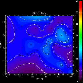
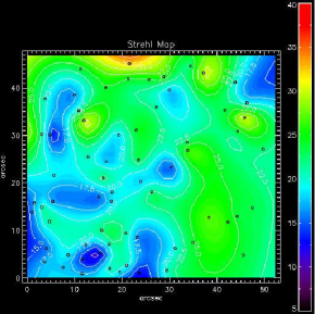
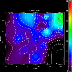
Figure 3: $K_{\rm s}$-band Strehl (%) maps for Fields 1, 2 and 3 (left to right, respectively). North is at the top, with east at the left.

3 Astrometric Calibration

Astrometric calibration of each field was undertaken using the Selman (1998) catalogue, recently recalibrated by Brian Skiff. These positions are dependent on the precision of the 2MASS/UCAC2 positions, combined with the plate-scale/seeing of the original New Technology Telescope (NTT) observations. The quoted precision on the new Skiff astrometry is $\sim$0$\aas@@fstack{\prime\prime}$1 (cf. the 0$\aas@@fstack{\prime\prime}$028/pixel delivered by MAD). Visual matches of stars between the Skiff catalogue and the MAD fields were used to define $\sim$40 well distributed astrometric standards in Fields 1 and 2. The astrometric calibration of Field 3, in which there are greater PSF variations, was achieved using 60 visually-matched stars.

4 Photometric calibration

Photometry was performed using standard daophot routines in iraf on the combined images. Due to the variations in the PSF delivered by the AO system across the field, PSF-fitting photometry was used, with the model PSF (penny2) allowed to vary quadratically across the fields. Roughly 30 bright, isolated stars were used to create a model PSF for each combined image, with neighbouring stars subtracted if they were contaminating the selected star. A fitting radius of (2$\times$FWHM)$-$1 pixels was found to provide the best fits. Objects with 1.5 $<$ sharpness $<-$1.5, or with $\chi<$ 4 (where $\chi$ is the root-mean-square of the residuals that remain) were rejected from the final catalogues to reject non-stellar objects, residual cosmic rays etc., as were objects with instrumental magnitude errors greater than 0.25^m.

4.1 Zero-point Calibrations

4.1.1 MAD vs. 2MASS

Sources from the Two Micron All Sky Survey (2MASS, Skrutskie et al., 2006) were identified in the MAD frames for photometric calibration. However, at the excellent angular resolution delivered by MAD many of the 2MASS ‘stars’ are resolved into asymmetric sources or multiple components (e.g. Fig. 3, Momany et al., 2008) . As such, only isolated, apparently single stars with 2MASS photometric qualities of either ‘A’, ‘B’, or ‘C’ in the relevant band were considered for calibration. This limited the number of 2MASS stars in each MAD field to eight or fewer for calibration.

Photometric zero points (ZPs) were determined (principally using ‘A’-rated 2MASS stars), with stars at the bright/faint ends of the MAD images omitted to exclude strongly-exposed stars in the MAD frames and poorly-exposed stars in 2MASS. The resulting ZPs are summarised in Table 2; we are somewhat at the mercy of small number statistics, not to mention the issues of stellar density and complex nebular emission in and around R136.

Table 2: Photometric zero-points obtained from the combined image method. Results are given for the $K_{\rm s}$-band images using 2MASS sources within the MAD frames, and using the HAWK-I commissioning data, in which the result for Field 2 was bootstrapped using overlapping stars with Field 1. The $H$-band results were obtained using 2MASS sources for Fields 1 and 3, with Field 2 again calibrated using overlapping stars with Field 1.

Band	Calibration	Field 1	Field 2	Field 3
$K_{\rm s}$	2MASS	26.78 $\pm$ 0.13	26.61 $\pm$ 0.45	26.95 $\pm$ 0.25
$K_{\rm s}$	HAWK-I	26.69 $\pm$ 0.08	27.04 $\pm$ 0.09	27.07 $\pm$ 0.11
$H$	2MASS	27.09 $\pm$ 0.14	27.27 $\pm$ 0.15	26.93 $\pm$ 0.08

4.1.2 MAD vs. HAWK-I

To investigate the quality of the calibrations we employed $K_{\rm s}$-band commissioning data from the VLT High Acuity Wide-field K-band Imager (HAWK-I, Pirard et al., 2004; Casali et al., 2006). HAWK-I is a wide-field, near-IR camera with four 2k x 2k Hawaii-2 detectors, covering a 7$\aas@@fstack{\prime}$5 square field at a pixel scale of 0$\aas@@fstack{\prime\prime}$106. Commissioning images of 30 Dor were obtained on 2007 October 3, using $Y$, $J$, $K_{\rm s}$ and Br$\gamma$ filters. The HAWK-I exposures were dithered around the centre of 30 Dor to build-up a complete mosaic for the region.

One $K_{\rm s}$-band HAWK-I array with a reasonable spatial overlap was selected for each MAD image. These frames were then reduced and analysed using the same methods as for the MAD images, i.e. using PSF-fitting photometry. There were $\sim$50 stars from 2MASS with ‘AAA’ $J$$H$$K_{\rm s}$ quality ratings in each of the HAWK-I frames. The resulting $K_{\rm s}$ ZPs were applied to all of the objects found in the image and a catalogue was created. A comparison of the HAWK-I magnitudes with those from 2MASS for the calibration stars is shown in Figure 4, with dispersions of $\pm$0.12, 0.16, and 0.21^m for Fields 1, 2 and 3, respectively.

These results provided a well-defined ZP between HAWK-I and 2MASS, which was then used to bootstrap the MAD ZPs from stars overlapping in the images. By comparing the instrumental magnitudes of 30 stars in the MAD frames with their corresponding HAWK-I values, new ZPs were calculated for each $K_{\rm s}$ MAD field. Note that the stars used were hand-picked to be isolated and well within the dynamic range of the MAD observations – using fainter sources from the MAD data would have pushed toward the sensitivity limits of the HAWK-I frames rather than providing improved calibration of the MAD data. The internal agreement of overlapping stars within the three HAWK-I frames used for calibration of the three MAD fields was found to be better than 0.1^m.

Figure 4: Residuals of the calibrated HAWK-I $K_{\rm s}$-band photometry compared with the 2MASS values. Field 1: open squares; Field 2: open triangles; Field 3: crosses.

Stars that appear in the overlap regions of the MAD fields were used as a double-check of the ZPs from the HAWK-I data. Fields 1 and 3 were in excellent agreement, while the ZP for Field 2 gave magnitudes that were 0.07^m brighter, although still within the calculated uncertainties; the ZP for Field 2 was corrected accordingly, resulting in $K_{\rm s}$-band magnitudes on a common system.

Unfortunately there were no matching HAWK-I observations in the $H$-band to employ a similar calibration method. Informed by the behaviour of the $K_{\rm s}$-band results, we adopt the 2MASS ZPs from Table 2 for Fields 1 and 3, which have much smaller standard deviations than found for Field 2. Instrumental magnitudes were then compared for stars overlapping between Fields 1 and 3 as done for $K_{\rm s}$; the resulting offsets were in excellent agreement with those expected from the ZPs from Table 2 (i.e., $\Delta$$H$$\sim$0.16^m). We then compared instrumental magnitudes for stars overlapping between Fields 1 and 2. These offsets were then used to calculate a new mean ZP for Field 2, which is within the quoted uncertainties from the 2MASS comparison, but has a much reduced error.

4.1.3 PSF Fitting on Individual Frames

If the PSF of a star varies subtly between different frames (as is likely with AO-corrected imaging) the resulting combined PSF may broaden slightly and be noisier. To investigate if this effect was the dominant source of our ZP uncertainties, we employed a second photometric method to see if we could improve the calibrations. We used PSF-fitting subtractions on the individual frames, then used Dr. Peter Stetson’s daomatch and daomaster packages to create a mean catalogue. This method potentially provides more precise PSF fitting, leading to improved fidelity of the final photometric catalogue. It also allows the user to set the number of frames in which a source must be detected for its inclusion in the final catalogue. This has the big advantage that objects in the dithered regions (previously discarded when the combined image is subset) can now be included, increasing the spatial extent of the final source catalogue, and also leads to fewer rejections of stars affected by cosmics or bad pixels in only one frame.

Table 3: Photometric zero-points obtained from the individual frame method. As in Table 2, the $K_{\rm s}$-band results are derived from HAWK-I, with the $H$-band results from 2MASS. In both cases Field 2 was calibrated using stars overlapping with Field 1.

Band	Field 1	Field 2	Field 3
$K_{\rm s}$	23.40 $\pm$ 0.07	23.62 $\pm$ 0.08	23.59 $\pm$ 0.11
$H$	24.45 $\pm$ 0.14	24.37 $\pm$ 0.14	24.33 $\pm$ 0.08

The uncertainties on the ZPs obtained from analysis of the individual frames were (effectively) unchanged compared to those found from our previous best efforts (see Table 3 cf. Table 2). This suggests that the uncertainties in the magnitudes of the calibration stars are dominanting those from the photmetric methods employed. A more tangible gain is the increased number of sources detected due to the retention of the dithered regions not observed in all frames (albeit with lower sensitivity). Following application of the ZP calibrations, a comparison between the combined-frame and individual catalogues was undertaken for each pointing/band, finding mean offsets less than 0.05^m in all six instances.

The ZPs adopted for calibration of the MAD fields for the final catalogue, created from the individual frames, are listed in Table 3. In summary, the $K_{\rm s}$-band ZPs were calibrated using HAWK-I, with Field 2 bootstrapped using overlapping stars in Field 1. The $H$-band ZPs were calibrated using 2MASS, also with Field 2 adjusted from comparisons with Field 1. Figure 5 compares the final MAD magnitudes with those of the HAWK-I calibration stars, with the dispersions around the mean quoted in Table 3.

Figure 5: Residuals of the calibrated MAD $K_{\rm s}$-band photometry from the individual frame method compared with the HAWK-I values for hand-picked reference stars (see text for details)

.

As an external check on the MAD magnitudes we compared our results for the 12 (visually-matched) overlapping stars in the NICMOS observations from Brandner et al. (2001). Nine of these stars were in Field 2 (with two only observed in the $H$-band due to the dither pattern), with the remaning three in Field 3. Accounting for the slight differences in the photometric filters (the HST data were transformed to the CTIO photometric system), the mean differences (MAD $-$ HST) and standard errors are in excellent agreement $\Delta$$H$ $=$ $-$0.05 $\pm$ 0.03 and $\Delta$$K_{\rm s}$ $=$ $-$0.04 $\pm$ 0.05 (std. err.).

4.2 Colour-magnitude diagrams

Colour-magnitude diagrams (CMDs) were created from catalogues from both photometric methods (i.e. from the combined and the individual frames), excluding objects within a radius of 2$\aas@@fstack{\prime\prime}$8 of the centre of R136, where crowding/blending become dominant.

The individual frame method yields an extra 600-1,000 objects in the CMDs compared to the analysis of the combined frames, mainly due to the increase in the effective field-of-view. When CMDs from the individual method are compared over the same spatial region as the combined CMD, Fields 2 and 3 contain slightly fewer objects, predominantly at fainter magnitudes, suggesting the individual frame method results in slightly diminished sensitivity. In contrast, Field 1 still contains fewer objects in the combined CMD, which is a legacy of a light leak down one side of the images that affected some of the MAD SD observations. Field 1 was the most affected by this light leak in our observations, with the image quality parameters in daophot rejecting more sources in analysis of the combined frame in this region than in the individual frames.

In addition to the inclusion of the dithered regions, the individual frame method reduces the random star-to-star uncertainties in the final catalogues. CMDs from the individual frame method are shown for all three fields in Figure 6. The location of the main-sequence is in good agreement for all three fields.

There is significant and variable extinction toward R136, with Andersen et al. (2009) adopting a median extinction of $A_{V}$ $=$ 1.85 for massive stars (M $=$ 7-20 M_⊙), corresponding to $A_{K}$ $\sim$ 0.21 (assuming, for the purposes of an order of magnitude estimate of the IR extinction, the standard galactic extinction law from Rieke & Lebofsky, 1985) and $A_{H}$ $\sim$ 0.32 (using the scaling from Indebetouw et al., 2005), yielding a relatively small near-IR extinction term of E($H$$-$$K_{\rm s}$) $=$ 0.11. Thus, the $H$$-$$K_{\rm s}$ colours from MAD will, in general, not be differentially reddened by much more than the photometric errors. CMDs were created for different radial bins using the combined catalogue from all three fields and these show no significant offset in the locus of the main sequence.

For Field 1 in Figure 6 we include the unreddened log$t$ $=$ 3.0 isochrone (effectively illustrative of the zero-age main sequence) from Lejeune & Schaerer (2001), adopting the tracks with the metallicity relevant to that of the LMC (i.e. those from Schaerer et al., 1993). Note that the offset from the MAD data is in agreement with the reddening estimated above.

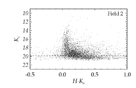
Figure 6: CMDs from the mean catalogues created from the individual frames method, excluding the central 2$\aas@@fstack{\prime\prime}$8 of R136. The dashed horizontal lines mark the 50% completeness level (cf. Figure 7) in the common regions included in all positional dithers. Overplotted in the Field 1 panel is the unreddened youngest isochrone (log$t$ $=$ 3.0) from Lejeune & Schaerer (2001), with the marked points indicating, from bright to faint magnitudes, initial masses of 60, 50, 25, 15, 9, 5, 3, and 2 M_⊙.

4.3 Photometric Completeness

Completeness tests were undertaken in both bands for all three fields. Using the starlist and addstar routines in iraf, 100 artificial stars with magnitudes varying from 14 to 24 were distributed uniformly across each combined (and subset) image. As before, PSF-fitting was performed, using the same settings and a penny2 model PSF which is allowed to vary across the field. Using the known positions of the added stars, the number recovered from the images within a two-pixel search radius was found. If more than one object was found within that small radius, the object with the smallest magnitude difference was considered the artificial star. Stars with magnitude differences of greater than $\pm$0.5^m were cut from the detected list, with the intention of excluding mistaken matches, or artificial stars which have been superimposed on genuine stars within the image (thus increasing its magnitude).

These tests were repeated 1,000 times, until 100,000 artificial stars had been added to each image. This gives a ratio of $\sim$30 to 50 artificial stars for each observed object. The ratio of artificial stars introduced to those detected was measured for each image, as shown in Figure 7. Field 2, which does not include R136 in the combined image, has a slightly more uniform completeness at brighter magnitudes while going slightly deeper in both bands.

The 50% completeness level in the $K_{\rm s}$-band frames is $K_{\rm s}$ $=$ 19.45 in Field 1, 19.85 in Field 2, and 18.90 in Field 3, corresponding to initial main-sequence masses of approximately 3.5, 2.8, and 4.7 M_⊙, respectively, when compared to the youngest isochrone from Lejeune & Schaerer (2001).

For Fields 1 and 3 the completeness was also found for both bands as a function of radius from the cluster (adopting 100 pixel radial bins), an example of which is shown in Figure 8. These radial completeness profiles are taken into account in construction of the radial luminosity profile in Section 6.

Figure 7: $H$ (upper panel) and $K_{\rm s}$(lower) completeness profiles for Fields 1, 2 and 3, as indicated.

Figure 8: $K_{\rm s}$-band radial completeness for Field 1. Each annulus has a width of 100 pixels (2$\aas@@fstack{\prime\prime}$8). ‘Radius 1’ refers to the radius closest to the cluster core.

5 Spitzer YSO candidates

From observations with the Spitzer Space Telescope, GC09 presented a catalogue of potential young stellar objects (YSOs) in the LMC. Prior to investigation of the luminosity profile of R136, we first investigated the seven candidate YSOs from their catalogue that are within the MAD fields. The Spitzer data were primarily obtained under the auspices of the Surveying the Agents of a Galaxy’s Evolution (SAGE) LMC survey (Meixner et al., 2006), but were also supplemented by smaller, more targeted programmes from the Spitzer archive.

Following initial colour cuts to exclude the majority of stars and background galaxies, GC09 investigated the nature of the candidate YSOs via inspection of their morphologies and spectral energy distributions, including comparisons at other wavelengths. This resulted in five categories for the colour-selected Spitzer sources: (1) evolved stars, (2) planetary nebulae, (3) background galaxies, (4) diffuse sources, and (5) ‘definite’, ‘probable’ and ‘possible’ YSO candidates. This is a somewhat different approach to the selection of candidate YSOs from the SAGE LMC survey by Whitney et al. (2008, see further discussion by GC09). Vaidya et al. (2009) have since compared the Spitzer data with archival HST H$\alpha$ images and new (seeing-limited) near-IR imaging, enabling more detailed description of the local environments around 82 of the YSOs from GC09.

The positional uncertainty on the Spitzer astrometry is approximately $\pm$0$\aas@@fstack{\prime\prime}$2 (Dr R. Gruendl, priv. comm.), but in the crowded environment of 30 Dor, one might expect that blended sources and nearby gas might lead to greater uncertainties. Indeed, the typical angular resolution of the Spitzer observations ranged from 1$\aas@@fstack{\prime\prime}$7 to 2$\aas@@fstack{\prime\prime}$0 over the four InfraRed Array Camera (IRAC) bands for the SAGE observations (Meixner et al., 2006). Thus, it is not surprising that, in the case of two of the ‘diffuse’ sources from GC09, we find apparent counterparts in the MAD images offset by a radius of approximately 1^′′.

In light of these positional uncertainties, there remains one candidate from GC09 which does not have an obvious close counterpart within a 2$\aas@@fstack{\prime\prime}$0 radius: the ‘diffuse’ candidate 053842.69 $-$690623.7. There is a faint source ($K_{\rm s}$ $=$ 18.1, $H$$-$$K_{\rm s}$ $=$ 0.39) at a distance of $\sim$0$\aas@@fstack{\prime\prime}$75, which is otherwise unremarkable; a brighter counterpart can be ruled out. We note that of the four Spitzer-IRAC bands, GC09 only reported magnitudes for this source at 4.5 and 8.0 $\mu$m, suggesting a less robust detection than for the other six sources discussed here which were detected in all four IRAC bands.

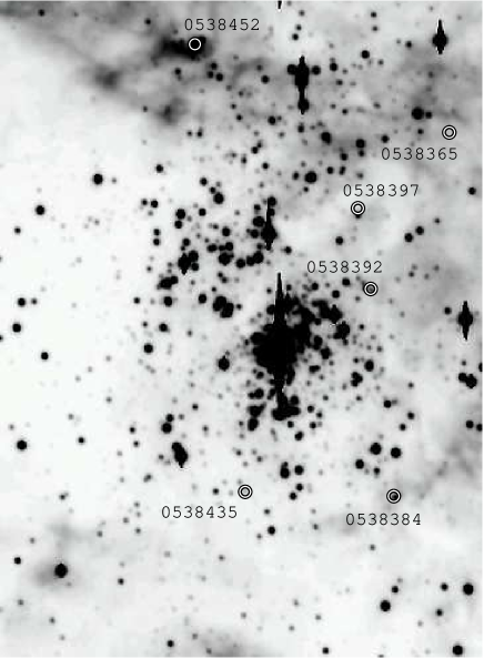
Figure 9: Location of the six YSOs from Gruendl & Chu (2009) with counterparts in the MAD images, overlaid on the $V$-band WFI image.

The remaining six YSO candidates are now discussed in turn, with their locations overlaid on the $V$-band WFI image in Figure 9 to illustrate their positions relative to R136. All except 053836.48 $-$690524.1 feature in the comparison by Vaidya et al. (2009), with four also within the (seeing-limited) near-IR imaging from Rubio et al. (1998, hereafter RBW98). Spitzer spectroscopy of three of these sources (053839.24 $-$690552.3, 053839.69 $-$690538.1 and 053845.15 $-$690507.9) was presented by Seale et al. (2009), with each classified in their ‘PE Group’, which are seen to display polycyclic aromatic hydrocarbon (PAH) emission features combined with fine-structure lines from ionised gas.

5.1 053836.48 $-$690524.1:

Reported as a ‘diffuse’ source by GC09, this object is on the western edge of the Field 2 images. Subset (5^′′ $\times$ 5^′′) $H$ and $K_{\rm s}$-band images are shown in Figure 10, in which the cross in the $H$-band image indicates the position from GC09 and the intensity scaling is the same in both bands. The circle (centred on the Spitzer position in the $H$-band image) indicates the typical angular resolution of IRAC in the SAGE survey, i.e. 1$\aas@@fstack{\prime\prime}$7 at 3.6 $\mu$m (Meixner et al., 2006). Just below the Spitzer position in the $H$-band image is a small cluster of bad pixels – the likely YSO counterpart is to the east and is more clearly seen in the $K_{\rm s}$-band image.

Apart from the obvious asymmetry in the $K_{\rm s}$-band image, we were somewhat cautious to match the MAD object to the GC09 source. However, Kim et al. (2007) also report a candidate YSO (their ‘30 Dor-15’, also from IRAC observations) that is only $\sim$0$\aas@@fstack{\prime\prime}$33 from the MAD counterpart, which has $K_{\rm s}$ $=$ 16.24, $H$ $-$ $K_{\rm s}$ $=$ 2.08.

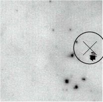
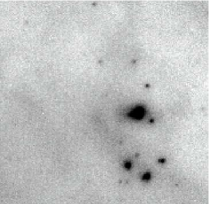
Figure 10: 053836.48 $-$690524.1: $H$- and $K_{\rm s}$-band 5${}^{\prime\prime}\times$5^′′ images (left- and right-hand panels, respectively), with north at the top, east at the left. The black cross marks the location of the Spitzer position for the YSO candidate, with the black circle representing the angular resolution of the IRAC data (1$\aas@@fstack{\prime\prime}$7 at 3.6 $\mu$m).

5.2 053838.35 $-$690630.4:

Classified as a ‘diffuse source’ by GC09, there is a potential counterpart ($K_{\rm s}$ $=$ 14.37 and $H$$-$$K_{\rm s}$ $=$ 0.35) in the MAD images at a distance of 1^′′ (Figure 15). The source appears to have an associated ‘plume’ of nebulosity which spirals to the south-west for at least 0$\aas@@fstack{\prime\prime}$5. This nebulosity can also be seen in the NICMOS image from Brandner et al. (2001, their 30Dor-NIC01 frame), but did not feature in their discussion.

The 2MASS $J$-band magnitude quoted by GC09 for this source is 13.93 (2MASS source: 053838.5-6906297). Overplotting the 2MASS catalogue on the MAD image reveals reasonable astrometric agreement (0$\aas@@fstack{\prime\prime}$2) considering the limited angular resolution of 2MASS, with upper limits of $H$ $>$ 12.88 and $K_{\rm s}$ $>$ 12.05 (i.e. ‘U’ rated).

This source also corresponds to IRSW-98 from RBW98 (which, in turn, is component ‘a’ of the knot comprising source W4 from Rubio et al., 1992), who found $K_{\rm s}$ $=$ 14.02 and $H$$-$$K_{\rm s}$ $=$ 0.45. Vaidya et al. (2009) note that this YSO is in a marginally-resolved H ii region, suggesting that the line contribution (at least in the $K_{\rm s}$-band) is likely contributing to the brighter magnitude from RBW98 compared to the MAD results.

5.3 053839.24 $-$690552.3:

The most likely YSO counterpart is at $\alpha$ $=$ 05^h 38^m 39$\aas@@fstack{s}$28, $\delta$ $=$ $-$69^∘ 05^′ 52$\aas@@fstack{\prime\prime}$60 (J2000, $\sim$0$\aas@@fstack{\prime\prime}$45 from the Spitzer position) and is the most immediately impressive counterpart in the MAD images (Figure 15). We find $K_{\rm s}$ $=$ 14.71 and $H$$-$$K_{\rm s}$ $=$ 0.42 for the star, as compared to $K_{\rm s}$ $=$ 13.91, $H$$-$$K_{\rm s}$ $=$ 0.61 from RBW98 (their source IRSW-118). The images from RBW98 were taken in typical seeing of 1^′′ so the two sources visible a the centre of Figure 15 will be strongly blended, leading to the brighter magnitude.

Particularly striking is the apparent bow-shock, most easily seen in the $K_{\rm s}$-band image. This is almost, but not quite, aligned with the core of R136 approximately 19$\aas@@fstack{\prime\prime}$5 away. Also of note in the same direction is R134/Brey 75 (Breysacher, 1981), classified as WN6(h) by Crowther & Smith (1997), at a distance of only 8^′′. To date, nothing is known regarding the spectral type of the two bright stars at the centre of the image (separated by $\sim$0$\aas@@fstack{\prime\prime}$33). This region clearly warrants more detailed investigation in the context of small-scale triggered star formation.

5.4 053839.69 $-$690538.1:

Classified as a ‘definite YSO’ by GC09, this object appears as a somewhat extended or embedded source in the $H$-band MAD image (Figure 15), with $K_{\rm s}$ = 13.75 and $H$$-$$K_{\rm s}$ = 3.37. This source corresponds to IRSW-127 from RBW98 (W9 from Rubio et al., 1992), for which they found $K_{\rm s}$ $=$ 13.91 and $H$$-$$K_{\rm s}$ $=$ 2.85.

The bright star 1$\aas@@fstack{\prime\prime}$2 to the south is P733/S206, for which $K_{\rm s}$ = 14.40 and $H$$-$$K_{\rm s}$ $=$ 0.16, suggesting it as a massive star (cf. the intrinsic colours from Martins & Plez, 2006). The strong contrast in the colours of the two stars is immediately obvious from the composite-colour image from RBW98 (their Figure 1), although they appear slightly blended. Blending could perhaps account for the photometric differences (which are in the expected direction), but RBW98 employed PSF-fitting methods so should be relatively robust to such effects at this separation – perhaps our efforts are somewhat limited by the apparent asymmetric flux to the south of the star.

5.5 053843.52 $-$690629.0:

Classified as a ‘possible YSO’ by GC09, the nearest spatial match is a source with $K_{\rm s}$ = 17.15 and $H$$-$$K_{\rm s}$ $=$ 1.01, as indicated in Figure 15. The adjacent object (0$\aas@@fstack{\prime\prime}$25 to the northeast) is P1064/S696, with $K_{\rm s}$ $=$ 16.87 and $H$$-$$K_{\rm s}$ $=$ 0.18, and for which the spectral type is unknown. This YSO source is not within the region observed by RBW98 but, interestingly, is noted by Vaidya et al. (2009) as being in a dark cloud and as comprising multiple YSOs in the Spitzer PSF, one with an optical counterpart in the H$\alpha$ HST images, and one without.

5.6 053845.15 $-$690507.9:

Classified as a ‘definite YSO’ by GC09, their published position is approximately 0$\aas@@fstack{\prime\prime}$4 north of P1222/S116/IRSN-101 (Parker, 1993; Selman, 1998, RBW98), which was classified as O3-6 V by Walborn & Blades (1997) from ground-based spectroscopy, later revised to O9 V(n)p by Walborn et al. (2002) from HST observations; 5${}^{\prime\prime}\times$5^′′ images of the region are shown in Figure 15. Note that P1222 was not used in the astrometric calibration of the MAD frames and yet its recovered position agrees with Skiff’s astrometry to better than two pixels.

This source lies within the dense nebular region referred to as ‘Knot 1’ by Walborn (1986), highlighted as young massive stars just emerging from their natal cocoons and imaged at optical and near-IR wavelengths with HST by Walborn et al. (1999, 2002). The relatively bright Spitzer magnitudes quoted by GC09 are in keeping with P1222 as the most plausible counterpart. Indeed, the spectral energy distribution shown in Figure 13 of GC09 reveals increased magnitudes bluewards of 1 $\mu$m, as well as redwards, consistent with a massive star with an IR excess. From the MAD images we find $K_{\rm s}$ $=$ 14.31 and $H$$-$$K_{\rm s}$ $=$ 0.13, as compared to $K_{\rm s}$ $=$ 14.45 and $H$$-$$K_{\rm s}$ $=$ 0.03 from the HST-NICMOS observations of Knot 1 by Brandner et al. (2001).

Vaidya et al. (2009) note the source as residing in a resolved H ii region and, on the basis of the H$\alpha$ luminosity (uncorrected for extinction) provide a lower bound on the inferred spectral type of the YSO of B0.5; evidently from the classification of Walborn & Blades, the star is slightly hotter.

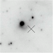
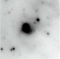
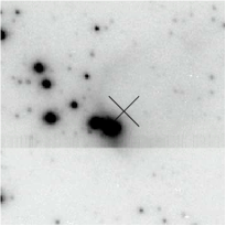
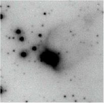
Figure 11: 053838.35 $-$690630.4: 5^′′ $\times$ 5^′′ $H$- and $K_{\rm s}$-band images.

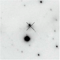
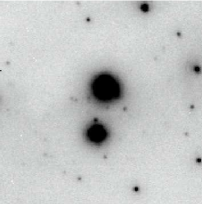
Figure 12: 053839.24 $-$690552.3: $H$- and $K_{\rm s}$-band. Note the particularly striking bow-shock feature in the $K_{\rm s}$ image.

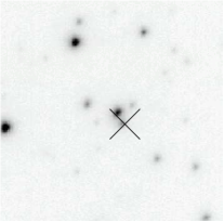
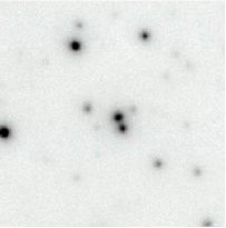
Figure 13: 053839.69 $-$690538.1: $H$- and $K_{\rm s}$-band.

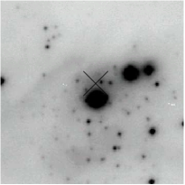
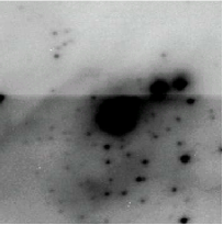
Figure 14: 053843.52 $-$690629.0: $H$- and $K_{\rm s}$-band.

Figure 15: 053845.15 $-$690507.9: $H$- and $K_{\rm s}$-band.

5.7 Spatial distribution and masses of YSOs

It is not surprising that five of the six YSO candidates discussed here lie to the north and west of R136 (Figure 9). This is the location of the ‘second generation’ of massive stars (Walborn et al., 1999, 2002), with significant molecular material still remaining (e.g. Werner et al., 1978; Johansson et al., 1998). The sixth source (053843.52 $-$690629.0) is spatially distinct from the regions of triggered star formation and is the most ambiguous of the YSOs discussed here; with M_K $\sim$ $-$1.4, it is also likely to be the lowest mass object.

The absolute $K_{\rm s}$-band magnitudes of our four brightest YSO counterparts are all bright, with M_K $\sim$ $-$3.75-4.75, suggesting that they are bona fide candidates for massive O- or early B-type stars, depending on the degree of obscuration/reddening. The most intriguing in this context is the very red source 053839.69 $-$6905381 which, given the uncertainties of the Spitzer astrometry, would certainly benefit from ground-based spectroscopy to elucidate its nature and its relationship with P733 nearby. Rubio et al. (2009) have recently reported a dense molecular cloud toward this source (their IRSW-127) suggesting that it may well be a massive star still heavily enshrouded in its natal cocoon.

6 Radial Luminosity Profile of R136

We now compare the radial luminosity profile for R136 from the MAD data, constructed using a combination of integrated-light measurements and star counts, with the optical HST results.

6.1 Integrated Light Profiles

Integrated-light measurements were used to investigate the innermost part of the radial luminosity profile in Fields 1 and 3. These sum the flux within annuli around the core, where the radius of each annulus is defined such that the total flux in each is approximately constant. An idl program was written specifically for this purpose, with standard daophot routines in iraf also used as a comparison. The idl program calculates the integrated light by re-sampling each image as a function of azimuth ($\phi$) and radius from the cluster centre, to enable a smoother, more robust calculation at smaller radii than possible with the (albeit small) sampling of the pixels – in practice the results are essentially the same as those obtained with iraf. These measurements adopt a constant sky value, which is defined well away from the cluster core.

To estimate the uncertainties in the integrated-light profile, each annulus is split into azimuthal sections and the density is calculated in each; the standard deviation of the results around each annulus then provide an estimate of the statistical uncertainties, provided the cluster is symmetric. However, visual inspection of the images shows that the cluster is not symmetric, particularly at larger radii (see Section 6.2.1), suggesting that the variations in the uncertainties are shaped by both statistical errors and asymmetric variations of the cluster.

The surface brightness profiles were then fit with Elson et al. (1987, EFF) cluster profiles of the form:

$$\mu(r)=\mu_{0}(1+\frac{r^{2}}{a^{2}})^{-\gamma/2},$$ (1)

where $a$ is the scale radius that defines where the flat inner part (the core) turns into a power-law profile with an index of $-\gamma$. The results are given in Table 4, both in terms of angular extent on the sky and in parsecs (adopting a distance modulus to the LMC of 18.5). The profile fits are shown in Figure 16, in which the lower three profiles are offset (in steps of two magnitudes) for clarity.

There is hardly any signature of a core, with the surface brightness profile fit by a power-law function over the full range of the data. The scale radius ($a$) obtained is effectively $\sim$ 0.1^′′ (0.025 pc) which is, in practice, the resolution limit of these data; i.e. 0.1^′′ provides an upper limit to the core radius. Both the results for the core and the slope of the power-law fit (i.e. $\gamma$ $\sim$ 1.6) are in good agreement with past optical HST results (Campbell et al., 1992; Hunter et al., 1995) and the new NICMOS results (Andersen et al., 2009).

Table 4: Structural parameters for R136 from EFF fits to the MAD integrated-light profiles. The italicised results are from fits to the combined luminosity profiles (see Section 6.3). For convenience, results are quoted in direct observables and their physical size in pc.

Field	$\mu_{0}$ [mag arcsec-2]	$a$ [′′]	$\gamma$	$r_{\rm c}$ [′′]
H F1	6.37 $\pm$ 0.12	0.13 $\pm$ 0.03	1.67 $\pm$ 0.15	0.15 $\pm$ 0.04
	6.36 $\pm$ 0.12	0.12 $\pm$ 0.02	1.57 $\pm$ 0.05	0.14 $\pm$ 0.03
H F3	6.59 $\pm$ 0.11	0.12 $\pm$ 0.03	1.58 $\pm$ 0.13	0.14 $\pm$ 0.03
	6.59 $\pm$ 0.11	0.12 $\pm$ 0.02	1.57 $\pm$ 0.05	0.13 $\pm$ 0.02
K F1	6.35 $\pm$ 0.14	0.13 $\pm$ 0.04	1.58 $\pm$ 0.15	0.15 $\pm$ 0.04
	6.35 $\pm$ 0.14	0.12 $\pm$ 0.02	1.48 $\pm$ 0.06	0.15 $\pm$ 0.03
K F3	6.39 $\pm$ 0.10	0.14 $\pm$ 0.03	1.63 $\pm$ 0.14	0.16 $\pm$ 0.04
	6.38 $\pm$ 0.11	0.12 $\pm$ 0.02	1.56 $\pm$ 0.06	0.15 $\pm$ 0.03
Field	$\mu_{0}$ [mag pc-2]	$a$ [pc]	$\gamma$	$r_{\rm c}$ [pc]
H F1	3.293 $\pm$ 0.121	0.031 $\pm$ 0.008	1.67 $\pm$ 0.15	0.035 $\pm$ 0.009
	3.282 $\pm$ 0.121	0.028 $\pm$ 0.005	1.58 $\pm$ 0.05	0.033 $\pm$ 0.006
H F3	3.517 $\pm$ 0.112	0.028 $\pm$ 0.007	1.58 $\pm$ 0.13	0.034 $\pm$ 0.008
	3.509 $\pm$ 0.112	0.027 $\pm$ 0.005	1.57 $\pm$ 0.06	0.032 $\pm$ 0.006
K F1	3.278 $\pm$ 0.136	0.031 $\pm$ 0.009	1.58 $\pm$ 0.15	0.037 $\pm$ 0.010
	3.269 $\pm$ 0.136	0.029 $\pm$ 0.006	1.48 $\pm$ 0.06	0.035 $\pm$ 0.007
K F3	3.316 $\pm$ 0.105	0.033 $\pm$ 0.008	1.63 $\pm$ 0.14	0.039 $\pm$ 0.010
	3.305 $\pm$ 0.105	0.030 $\pm$ 0.006	1.56 $\pm$ 0.06	0.036 $\pm$ 0.007

Figure 16: EFF fits to the MAD integrated-light profiles, with the $K_{\rm s}$- and $H$-band (Field 3) profiles shifted to fainter magnitudes for clarity.

6.2 Star Counts

Star counts in annuli around the core were used to calculate the radial luminosity profile in the regions beyond $r$ $=$ 2$\aas@@fstack{\prime\prime}$8. Stars were binned such that a similar number of objects were included per annulus, as suggested by Maíz Apellániz & Úbeda (2005). The stars were binned as a function of radius and magnitude and completeness terms were calculated. As the core is off-centre in each frame, area correction terms were applied to correct the densities if part of a given annulus extended past the edge of an image.

The radial completeness tests (e.g. Figure 8) reveal, not unsurprisingly, that the first couple of annuli beyond $r$ $=$ 2$\aas@@fstack{\prime\prime}$8 are also strongly affected by crowding, and are thus subject to greater uncertainties than in the outer regions. The 50$\%$ completeness level in the third radial bin was adopted as the faint limit for construction of the profiles from the star counts, corresponding to a faint magnitude limit in each field in the range of 18.5-18.8^m, equating to a main-sequence mass of $\sim$5 M_⊙. The innermost bins were not included in construction of the final combined profile.

6.2.1 Azimuthal Density Variations

To investigate the apparent asymmetry in R136 more quantitatively, we calculated the azimuthal density variation beyond the central 2$\aas@@fstack{\prime\prime}$8. An idl program was used to split the images into angular slices, each containing approximately equal numbers of stars (after completeness corrections were applied). Similar techniques have been used recently to investigate the structure and asymmetries seen in lower-mass Galactic clusters (e.g. Gutermuth et al., 2005; Gutermuth et al., 2009).

Due north from the cluster core was set as $\phi$=0^∘, increasing anti-clockwise (increasing towards the east), with the outer radius set by the distance from the cluster core to the northern edge of Field 1. This enables a near complete azimuthal sweep in the combined $H$-band images of Fields 1 and 3 (i.e. not the full extent of those shown in Figure 2). An iterative routine was used to define an azimuthal slice in each image (increasing by 1^∘ each loop), which summed the star counts in that slice and corrected for the incompleteness (down to 50%). Once 200 stars are obtained, the routine determines the area covered by each slice, calculates the density, and then moves on to define the next slice.

The azimuthal variation around R136 (with $r_{\rm max}$ = 28$\aas@@fstack{\prime\prime}$0, $\equiv$ 1,000 pixels) is clearly seen in Figure 18, demonstrating that this region is far from symmetric, with a local minimum around $\phi$ $=$ 90^∘. Note that the $H$-band densities are larger as a consequence of the deeper images compared to the $K_{\rm s}$-band observations (see Figure 7). The exact densities are sensitive to the completeness threshold employed, so similar calculations were undertaken for completeness cuts of 30, 40, and 60% (with the results for 40% shown in Figure 18). While there are variations in the exact densities as a function of $\phi$ (partly because the different depths yield slices which vary in size in terms of $\phi$), the overall trend remains the same.

Adopting a distance modulus of 18.5 to the LMC, $r$ = 28$\aas@@fstack{\prime\prime}$0 corresponds to a projected radius of 6.8 pc. Similar trends in the azimuthal profiles are also seen adopting outer radii of 600 and 800 pixels (4.1 and 5.4 pc, respectively). At smaller radii incompleteness effects become more significant (cf. Figure 8) and it is harder to characterise the asymmetry meaningfully. Superficial inspection of Figure 2 from Massey & Hunter (1998) suggests similar asymmetries in the inner region, with luminous stars appearing to be more numerous in the eastern half of the central 4$\aas@@fstack{\prime\prime}$55 $\times$ 4$\aas@@fstack{\prime\prime}$55 HST image. However, we also note that the most luminous, massive stars will likely have a different relaxation time to the lower-mass population.

Figure 17: Azimuthal density profiles for a maximum radius of 28$\aas@@fstack{\prime\prime}$0 from the core of R136 and a completeness cut-off of 50%, demonstrating that the cluster is not relaxed over a $\sim$7 pc scale. Due north from the cluster centre corresponds to $\phi$ = 0^∘.

Figure 18: As Figure 18, but with a completeness cut-off of 40%.

6.3 Combined Radial Profile

The overlap region between the profiles from the two methods was used to convert (and normalise) the star counts into surface brightness – a reasonable approach provided there is no evidence of mass segregation in the cluster (as claimed by Hunter et al., 1995, although Brandl et al. 1996 argued to the contrary). The average offset in the overlap region was found from interpolation between the two profiles, re-sampled to an evenly sampled grid of radial bins to avoid a bias toward smaller radii (at which the bins are smaller) and excluding the innermost bin from the star counts profile (to be less sensitive to completeness corrections). The offset was then used to convert the star counts into a magnitude density, yielding a combined profile.

EFF fits to the combined profile are shown in Figures 21 and 21, with the fit parameters given in italics in Table 4. Meaningful errors on the star counts are hard to estimate due to the difficulty of attributing uncertatinties to the completeness corrections (i.e. blending/crowding effects) and the area corrections (i.e. cluster asymmetries), so we adopt a conservative error of $\pm$10% of the density values for each bin, which are then scaled as per the profile into a magnitude density. Note that the slopes of the fits are nearly identical to those from analysis of the integrated-light profile, although the results are very slightly shallower.

Figure 19: EFF fits to the combined MAD profiles for Field 1 (with the $K_{\rm s}$-band profile offset to fainter magnitudes for clarity).

Figure 20: EFF fits to the combined MAD profiles for Field 3 (with the $K_{\rm s}$-band profile offset to fainter magnitudes).

Figure 21: Profile fits to the HST optical data from Mackey & Gilmore (2003), with the $I$-band profile offset to fainter magnitudes.

There are striking differences between the EFF fits to the MAD data and the optical results from Mackey & Gilmore (2003). We also fitted EFF profiles to the data from Mackey & Gilmore, with it truncated to the outer radius of the MAD data. However, without measurements closer to the core it is difficult to obtain a meaningful comparison for $\mu_{0}$ and $a$. Their inner data points suggest a somewhat steeper turnover, with Mackey & Gilmore reporting $\gamma$ $=$ 2.43 $\pm$ 0.09 for their inner EFF component, but the integrated-light MAD measurements at $r$ $<$ 1^′′ rule out such a slope in the near-IR. Most relevantly, fits to the slope of the optical data yield $\gamma$ $=$ 1.80 $\pm$ 0.10 in both the $V$ and $I$ bands, in reasonable agreement with the MAD data, as illustrated in Figure 21. Note the presence of the bump (or dent) noted by both Meylan (1993) and Mackey & Gilmore (2003), at a radius of approximately 10^′′. For comparison, McLaughlin & van der Marel (2005) found $\gamma\,=\,$2.05 from fits to the full range of the HST data

A value of $\gamma$ $=$ 1.65 $\pm$ 0.08 was also found for the slope of the number density profile for stars brighter than M_V $=$ $-$5 by Moffat et al. (1994). The extension of the power-law out to $\sim$ 10 pc makes R136 a good example of clusters with an extended halo – not all young clusters have such a halo, as illustrated by Moffat et al. (1994) through a comparison with NGC 3603, which lacks bright stars beyond $\sim$ 1 pc. Maíz Apellániz (2001) shows several extra-galactic examples of clusters with and without an extended halo. The origin of such halos in some clusters compared to those without remains unclear at present.

6.4 Discussion

6.4.1 Structural parameters of R136

In summary, we find slopes of $\gamma\,\leq\,$2 from EFF fits to the near-IR luminosity profile of R136. If extrapolated to infinity such a profile would have infinite mass, so this can not extend to very large radii as the bulk of the mass would then be far from the core. It remains to be seen what the origin of these very shallow profiles is, although Larsen (2004) found that shallower profiles were more common in the younger members of their extragalactic cluster sample, and that $\gamma$ appears to increase with age. The development of a core and the reduction of the central density with age is likely the result of mass loss by stellar evolution and heating by binaries in the centre (Takahashi & Portegies Zwart, 2000).

Due to the very young age of R136 its density profile could be related to the formation process of the cluster, i.e. while it is still in its earliest stages of evolution we might see the imprint of the parent molecular cloud. Molecular clouds are approximately isothermal spheres in which, with $\gamma$ $=$ 1 (i.e. $\gamma_{\rm 3D}$ $=$ 2), the density scales as $\rho$ $\propto$ $r^{-2}$ (e.g. McGlynn, 1984). For example, Huff & Stahler (2006) found that the Orion Nebula Cluster (with an age of $\sim$1 Myr) can be well approximated by a power-law profile with $\gamma\,=\,$1. Alternatively, the dissipationless collapse of a (gas free) stellar system also results in a power-law density profile, and possibly a core. The size of the core and the slope of the density profile depends mainly on the virial temperature in the initial configuration (McGlynn, 1984). For a cold collapse, i.e. zero initial velocities of the stars, McGlynn found $\sim\,$1.5$\,<\,\gamma\,<\,\sim\,$2, with a core size of almost zero. The ‘warmer’ the initial conditions, the steeper the density profile and the larger the size of the core in the final configuration. So the observed density profile in R136 could also be the result of a cloud collapse, with star formation occurring in the early phases of the collapse, such that the dynamical interactions between the stars determine the properties of the cluster.

Hunter et al. (1995) found no evidence for mass segregation in R136. Andersen et al. (2009) also ruled it out for $r$ $>$ 3 pc ($\equiv$12$\aas@@fstack{\prime\prime}$4), finding no evidence for the flattening of the IMF below 2 M_⊙ reported by Sirianni et al. (2000). An early AO study of one 12$\aas@@fstack{\prime\prime}$8 $\times$ 12$\aas@@fstack{\prime\prime}$8 quadrant of R136 by Brandl et al. (1996) sampled a similar mass range to the MAD data, and found evidence of mass segregation above 12 M_⊙. Whether the MAD data shows effects of the more massive stars being preferentially in the core will be addressed elsewhere, but if evidence for mass segregation were found in the inner 3 pc, then the core radius derived here would be somewhat smaller than the ’primordial’ radius.

6.4.2 Structure at larger radii

Evidence for a second component in the near-IR profiles is less compelling than in the optical data, and we do not invoke a second component in our EFF fits. There is tentative evidence in Field 1 for a ‘dent’ at comparable radius to the optical data (Figure 21 cf. Figure 21), but the data for Field 3 are fit more cleanly by a single-component profile (Figure 21). Unfortunately the MAD data do not lend themselves to analysis of the integrated light out to larger radii. While the ‘stitching together’ of the two parts of the profile can influence the appearance of the combined profile, exclusion of one or two bins in the overlap region when combining them has very little influence on the EFF results. Indeed, now armed with knowledge of the minimal core, the EFF fits to the optical data are well matched at larger radii.

The lack of a second component is interesting since theoretical explanations for bumps (or halos) around young dense clusters (e.g. Bastian & Goodwin, 2006) should be independent of the wavelength in which the profile is constructed. The temptation is to attribute the past (two-component) results to variable extinction in the optical images. From the optical image of R136 (Figure 2) there is a notable ‘void’ to the north-east (running from north-west to south-east) at $r$ $\sim$ 10^′′, suggesting that differential extinction could be a prime suspect. We also note that more prosaic reasons (using circular annuli to determine the luminosity profiles in elliptical clusters) are now also being suggested to account for apparent breaks in density profiles in other clusters (Perina et al., 2009).

In this context, the asymmetric structure seen in Figure 18 must contribute strongly – almost certainly leading to the differences seen in the outer regions in Figures 21 and 21. Further support of this hypothesis is provided by inspection of the original Wide Field Planetary Camera 2 (WFPC2) images used by Mackey & Gilmore. R136 was located slightly off-centre in the Planetary Camera detector, with the Wide-Field Cameras primarily sampling the region east of R136, i.e. Field 1 observed with MAD. Interestingly, Andersen et al. (2009) only fit their EFF profile to the inner 2 pc ($\equiv$8$\aas@@fstack{\prime\prime}$25), noting in the caption to their Figure 12 that the presence of individual bright stars introduces ‘the jitter in the surface brightness profile’, hinting at the arguments that we advance here.

Such deviations from symmetry are not surprising in such a massive, intricate, multi-population and, as yet, seemingly unrelaxed star-formation region. This point is reinforced by the identification of (at least) five distinct populations in 30 Dor by Walborn & Blades (1997), three of which are sampled by the MAD observations: the central ‘Carina Phase’ (rich in early O-type stars and including R136), an older ‘Scorpius OB1 Phase’ of early-type supergiants throughout the central field, and a young (likely triggered) ‘Orion Phase’ to the north and west, mostly embedded in the gaseous filaments visible in Figure 2 and partially observed by Field 2. The stars associated with these populations in the region immediately around R136 are neatly illustrated by Figures 3 and 4 from w86 – their distribution is far from uniform, illustrative of the asymmetries shown in Figure 18.

The twin populations around R136 invite the question of their formation history. Is the Sco OB1 Phase simply the remaining ‘field’ population, dispersed from a previous star-formation event? Are the younger, more massive Carina Phase stars formed locally, or are they ejected members of R136? The answer to the latter question is most likely a combination of both. Without comprehensive stellar and gas dynamics of the different populations in 30 Dor we are limited to speculation at the present time, but this is one of the principal motivations for the VLT-FLAMES Tarantula Survey (Evans et al., 2010), which has obtained multi-epoch optical spectroscopy for over 1,000 stars and will address these points.

The formation history of these ‘halo’ stars goes to the heart of the theory of infant mortality, where deviations from EFF profiles in M82-F, NGC 1569-A and NGC 1705-1 were argued by Bastian & Goodwin (2006) to arise from rapid gas removal in clusters undergoing violent relaxation. Note that the HST profile from Mackey & Gilmore (2003) extends beyond a radius of 60^′′, thus also sampling the triggered generation as well as the halo around R136, i.e. some of the excess light reported by Mackey & Gilmore (and, by inference, by Bastian & Goodwin) is likely attributable to ejected stars, but that triggered star formation also contributes.

To echo the sentiment of Walborn & Blades (1997), the central 2^′ of 30 Dor observed with MAD corresponds to a physical size of $\sim$30 pc. If one projects this to a distance of 10 Mpc, the same structures would all be contained within $\sim$0$\aas@@fstack{\prime\prime}$5. This reinforces the need to take potential cluster asymmetries and triggered star-formation into account when interpreting the radial luminosity profiles of distant unresolved clusters.

The MAD data have provided us with a truly unique view of the central region of 30 Doradus. In the broader context, the delivery of impressive image quality and stability across wide fields (compared to classical AO observations) is very encouraging in advance of future multi-laser, MCAO systems on 8-m class telescopes, and the development of wide field, AO-corrected, imagers and spectrometers for the E-ELT.

acknowledgments: The data presented here were obtained during the MAD Science Demonstration campaign (package name MADD-SD-EV, ID 96408). and we are indebted to the MAD team of Paola Amico, Enrico Marchetti and Johann Kolb (with particular thanks to Johann for the Strehl maps). MAC acknowledges financial support from the Science and Technology Facilities Council (STFC). We thank the referee, Morten Andersen, and Nolan Walborn and Jesus Maíz Apellániz for their suggestions and comments which improved this article. We also thank the HAWK-I instrument and commissioning teams for making the 30 Dor frames available and John Pritchard for his advice with those images, Robert Gruendl for correspondence regarding the YSO catalogue, Yazan Al Momany for a fateful conversation over coffee in Santiago and subsequent advice on the individual frames method, and Peter Stetson for making his routines available to us.

References

- Amorim et al. (2006) Amorim A., Lima J., Alves J. et al.., 2006, Proc. SPIE, 6269, 164
- Andersen et al. (2009) Andersen M., Zinnecker H., Moneti A. et al.., 2009, ApJ, 707, 1347
- Bastian et al. (2008) Bastian N., Gieles M., Goodwin S. P. et al.., 2008, MNRAS, 389, 223
- Bastian et al. (2005) Bastian N., Gieles M., Lamers H. J. G. L. M., Scheepmaker R. A., de Grijs R., 2005, A&A, 431, 905
- Bastian & Goodwin (2006) Bastian N., Goodwin S. P., 2006, MNRAS, 369, L9
- Baumgardt & Kroupa (2007) Baumgardt H., Kroupa P., 2007, MNRAS, 380, 1589
- Bosch et al. (2001) Bosch G., Selman F., Melnick J., Terlevich R., 2001, A&A, 380, 137
- Bouy et al. (2008) Bouy H., Kolb J., Marchetti E. et al.., 2008, A&A,, 477, 681
- Brandl et al. (1996) Brandl B., Sams B. J., Bertoldi F. et al.., 1996, ApJ, 466, 254
- Brandner et al. (2001) Brandner W., Grebel E. K., Barbá R. H., Walborn N. R., Moneti A., 2001, AJ, 122, 858
- Breysacher (1981) Breysacher J., 1981, A&AS, 43, 203
- Campbell et al. (1992) Campbell B., Hunter D. A., Holtzman J. A. et al.., 1992, AJ, 104, 1721
- Campbell et al. (2008) Campbell M. A., Evans C. J., Ascenso J. et al.., 2008, Proc. SPIE, 7015, 61
- Casali et al. (2006) Casali M., Pirard J.-F., Kissler-Patig M. et al.., 2006, Proc. SPIE, 6269, 29
- Crowther & Smith (1997) Crowther P. A., Smith L. J., 1997, A&A, 320, 500
- de Marchi et al. (1993) de Marchi G., Nota A., Leitherer C., Ragazzoni R., Barbieri C., 1993, ApJ, 419, 658
- Elson et al. (1987) Elson R. A. W., Fall S. M., Freeman K. C., 1987, ApJ, 323, 54
- Evans et al. (2010) Evans C. J., Bastian N., Beletsky Y. et al., 2010, in de Grijs R., Lépine J. R. D., eds, Star Clusters – Proceedings IAU Symposium No. 266, arXiv:0909.1652, p. 35
- Fall et al. (2005) Fall S. M., Chandar R., Whitmore B. C., 2005, ApJ, 631, L133
- Goodwin & Bastian (2006) Goodwin S. P., Bastian N., 2006, MNRAS, 373, 752
- Gruendl & Chu (2009) Gruendl R. A., Chu Y.-H., 2009, ApJS, 184, 172 [GC09]
- Gutermuth et al. (2009) Gutermuth R. A., Megeath S. T., Myers P. C. et al., 2009, ApJS, 184, 18
- Gutermuth et al. (2005) Gutermuth R. A., Megeath S. T., Pipher J. L. et al., 2005, ApJ, 632, 397
- Huff & Stahler (2006) Huff E. M., Stahler S. W., 2006, ApJ, 644, 355
- Hunter et al. (1995) Hunter D. A., Shaya E. J., Holtzman et al., 1995, ApJ, 448, 179
- Hunter et al. (1997) Hunter D. A., Vacca W. D., Massey P., Lynds R., O’Neil E. J., 1997, ApJ, 113, 1691
- Indebetouw et al. (2005) Indebetouw R., Mathis J. S., Babler B. L., et al. 2005, ApJ, 619, 931
- Johansson et al. (1998) Johansson L. E. B., Greve A., Booth R. S. et al.., 1998, A&A, 331, 857
- Kim et al. (2007) Kim H., Kim S., Bak J.-Y. et al., 2007, ApJ, 669, 1003
- Lada & Lada (2003) Lada C. J., Lada E. A., 2003, ARA&A, 41, 57
- Larsen (2004) Larsen S. S., 2004, A&A, 416, 537
- Lejeune & Schaerer (2001) Lejeune T., Schaerer D., 2001, A&A, 366, 538
- Mackey & Gilmore (2003) Mackey A. D., Gilmore G. F., 2003, MNRAS, 338, 85
- Maíz Apellániz (2001) Maíz Apellániz J., 2001, ApJ, 563, 151
- Maíz Apellániz & Úbeda (2005) Maíz Apellániz J., Úbeda L., 2005, ApJ, 629, 873
- Marchetti et al. (2007) Marchetti E., Brast R., Delabre B. et al.., 2007, Msngr, 129, 8
- Martins & Plez (2006) Martins F., Plez B., 2006, A&A, 457, 637
- Massey & Hunter (1998) Massey P., Hunter D. A., 1998, ApJ, 493, 180
- McGlynn (1984) McGlynn T. A., 1984, ApJ, 281, 13
- McLaughlin & van der Marel (2005) McLaughlin D. E., van der Marel R. P., 2005, ApJS, 161, 304
- Meixner et al. (2006) Meixner M., Gordon K. D., Indebetouw R. et al.., 2006, AJ, 132, 2268
- Melnick (1985) Melnick J., 1985, A&A, 153, 235
- Meylan (1993) Meylan G., 1993, in Smith G. H., Brodie J. P., eds, The globular clusters-galaxy connection Astronomical Society of the Pacific (ASP) Conference Series, Vol. 48, p. 588
- Moffat et al. (1994) Moffat A. F. J., Drissen L., Shara M. M., 1994, ApJ, 436, 183
- Momany et al. (2008) Momany Y., Ortolani S., Bonatto C., Bica E., Barbuy B., 2008, MNRAS, 391, 1650
- Noyola & Gebhardt (2007) Noyola E., Gebhardt K., 2007, AJ, 134, 912
- Parker (1993) Parker J. W., 1993, AJ, 106, 560
- Parker & Garmany (1993) Parker J. W., Garmany C. D., 1993, AJ, 106, 1471
- Perina et al. (2009) Perina S., Barmby P., Beasley M. A. et al.., 2009, A&A, 494, 933
- Pirard et al. (2004) Pirard J.-F., Kissler-Patig M., Moorwood A. et al.., 2004, Proc. SPIE, 5492, 1763
- Rieke & Lebofsky (1985) Rieke G. H., Lebofsky M. J., 1985, ApJ, 288, 618
- Rubio et al. (1998) Rubio M., Barbá R., Walborn N. R. et al.., 1998, AJ, 116, 1708 [RBW98]
- Rubio et al. (2009) Rubio M., Paron S., Dubner G., 2009, A&A, 505, 177
- Rubio et al. (1992) Rubio M., Roth M. R., García J., 1992, A&A, 261, L29
- Schaerer et al. (1993) Schaerer D., Meynet G., Maeder A., Schaller G., 1993, A&AS, 98, 523
- Seale et al. (2009) Seale J. P., Looney L., Chu Y.-H. et al.., 2009, ApJ, 699, 150
- Selman (1998) Selman F., 1998, A&A, 341, 98
- Sirianni et al. (2000) Sirianni M., Nota A., Leitherer C., De Marchi G., Clampin M., 2000, ApJ, 533, 203
- Skrutskie et al. (2006) Skrutskie M. F., Cutri R. M., Stiening R. et al.., 2006, AJ, 131, 1163
- Takahashi & Portegies Zwart (2000) Takahashi K., Portegies Zwart S. F., 2000, ApJ, 535, 759
- Vaidya et al. (2009) Vaidya K., Chu Y.-H., Gruendl R. A., Chen C.-H. R., Looney L. W., 2009, ApJ, 707, 1417
- Walborn (1986) Walborn N. R., 1986, in De Loore C. W. H. e. a., ed., Luminous Stars and Associations in Galaxies – Proceedings IAU Symposium No. 116 Dordrecht, D. Reidel Publishing Co., p. 185
- Walborn et al. (1999) Walborn N. R., Barbá R. H., Brandner W. et al.., 1999, AJ, 117, 225
- Walborn & Blades (1997) Walborn N. R., Blades J. C., 1997, ApJS, 112, 457
- Walborn et al. (2002) Walborn N. R., Maíz-Apellániz J., Barbá R. H., 2002, AJ, 124, 1601
- Werner et al. (1978) Werner M. W., Becklin E. E., Gatley I. et al.., 1978, MNRAS, 184, 365
- Whitney et al. (2008) Whitney B. A., Sewilo M., Indebetouw R. et al.., 2008, AJ, 136, 18