TTP10-12
Narrow resonances studies with the radiative return method

Abstract

Using the radiative return method, experiments at high luminosity electron-positron colliders allow to explore the kaon and the pion form factors in the time-like region up to fairly high energies. This opens the possibility to study kaon and pion pair production at and around the narrow resonances $J/\psi$ and $\psi(2S)$ and explore the interference between electromagnetic and hadronic amplitudes. Parameterizations of charged and neutral kaon as well as pion form factors are derived, which lead to an improved description of the data in the region of large invariant masses of the meson pair. These form factors are combined with the hadronic couplings of charged and neutral kaons to $J/\psi$ and $\psi(2S)$ and implemented into the Monte Carlo generator PHOKHARA, which is now, for the first time, able to simulate the production of narrow resonances and their decay into kaon, pion and muon pairs.

I Introduction

New and precise measurements of the cross section for electron-positron annihilation into hadrons have been performed during the past years which were based on the method of ”Radiative Return” Zerwas ; Binner:1999bt . Exclusive reactions, specifically two-body final states like $\pi^{+}\pi^{-}$ :2008en ; :2009fg , $p\bar{p}$ Aubert:2005cb or $\Lambda\bar{\Lambda}$ Aubert:2007uf and three- Aubert:2004kj ; Aubert:2007ym and four-meson final states Aubert:2005eg ; Aubert:2007ur have been explored. An important ingredient in these analyzes was and is the simulation of all these reactions through a Monte Carlo generator. In a first step, the generator EVA was developed Binner:1999bt ; Czyz:2000wh , which is based on leading order matrix elements combined with structure function methods for an improved treatment of initial state radiation. Subsequently the complete next-to-leading order (NLO) QED corrections were evaluated Rodrigo:2001jr ; Kuhn:2002xg and implemented into the generator PHOKHARA Rodrigo:2001kf ; Czyz:2002np ; Czyz:PH03 ; Nowak ; Czyz:PH04 ; Czyz:2004nq ; Czyz:2005as ; Czyz:2007wi ; Czyz:2008kw , which is now available for a variety of exclusive final states. (For a recent review of theoretical and experimental results see e.g. Actis:2009gg .) B-meson factories, operating at energies around 10 GeV and with high luminosity, allow to explore hadronic final states with relatively large invariant masses, up to 3 GeV and beyond. Therefore, the narrow resonances $J/\psi$ and $\Psi(2S)$ can be studied through the radiative return, in particular in decay channels of low multiplicity, leptonic ones like $\mu^{+}\mu^{-}$ Aubert:2003sv , or two-body hadronic modes like $\pi^{+}\pi^{-}$, $K^{+}K^{-}$, $K^{0}\bar{K}^{0}$ or $p\bar{p}$ Aubert:2005cb . The signal is identified with the help of a very good mass resolution and particle identification in the resonance region.

For an analysis exploiting the large statistics, the inclusion of radiative corrections from initial- and final-state radiation (ISR and FSR) is mandatory, since it affects the cross section and the line shape of the resonance. For the simulation of hadronic final states both the electromagnetic contribution, i.e. a parameterization of the form factor, and the strength of the direct coupling of the resonance to the hadrons are required. The latter is absent for final states with positive G-parity ($2\pi$, $4\pi$, … ) but non-vanishing e.g. for $K\bar{K}$, $3\pi$ or final states with baryons. On the other hand, a careful analysis of the resonance line shape in the various channels would allow a model-independent determination of the direct coupling and of the form factors close to resonance Czyz:2009vj ; Seth:Jphi ; Yuan:2003hj ; Rosner:1999zm ; Suzuki:1999nb ; LopezCastro:1994xw ; Milana:1993wk .

With this motivation in mind we reanalyze the pion and kaon form factors with emphasis on the region above the $\rho$-resonance. The basic ingredients are very similar to those employed in an earlier study Bruch . However, additional assumptions are required to properly describe the different resonance-like structures in the energy region between 1 GeV and 3 GeV. The details of this model and its parameters are described in sections II and III for pions and kaons, respectively. The new implementation of these modes into PHOKHARA, which includes, as before, NLO ISR and FSR, is presented in Section IV. Section V is concerned with the implementation of the narrow resonances in the channels $\mu^{+}\mu^{-}$, $\pi^{+}\pi^{-}$, $K^{+}K^{-}$ and $K^{0}\bar{K}^{0}$. Hadronically and electromagnetically induced amplitudes are included, together with the radiative corrections from ISR and FSR. Section VI contains a brief summary and our conclusions.

II The pion form factor

For a realistic generation a model for the electromagnetic form factor is required. The ansatz presented in Bruch was published before the CLEO-c measurement of the form factor in the vicinity of the $\psi(2S)$ resonance Pedlar:2005sj and underestimates the experimental result significantly. The same applies to the model predictions at $J/\psi$ as compared to the pion form factor calculated in Milana:1993wk from $B(J/\psi\to\pi^{+}\pi^{-})$ and $B(J/\psi\to e^{+}e^{-})$ decay rates.

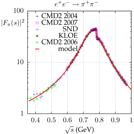
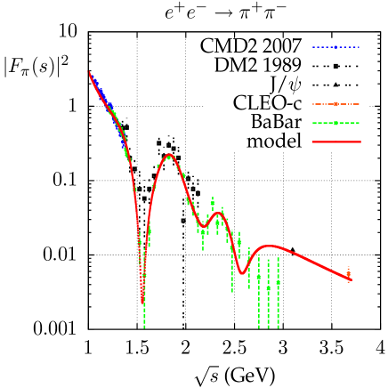
Figure 1: (color online) The experimental data Bisello:1988hq ; :2009fg ; Akhmetshin:2003zn ; Akhmetshin:2006bx ; Akhmetshin:2006wh ; Achasov:2005rg ; Aulchenko:2006na ; :2008en ; Pedlar:2005sj compared to the model fits results (see text for details). The form factor at $J/\psi$ comes from its theoretical extraction Milana:1993wk ; Amsler:2008zz from the data.

To accommodate the new data, the updated model ansatz for the pion form factor is taken similarly to Bruch

$$F_{\pi}(s) = \left[\sum\limits_{n=0}^{N}c_{\rho_{n}}^{\pi}BW_{\rho_{n}}(s)\right]_{fit}$$ (1)

$$+\left[\sum\limits_{n=(N+1)}^{\infty}c_{\rho_{n}}^{\pi}BW_{\rho_{n}}(s)\right]_{dQCD}\ ,$$

however, with different set of parameters. Those of the first $N+1$ $\rho$ radial excitations are fitted and the rest is taken from the “dual QCD model” Dominguez:2001zu . It is necessary to take $N=5$ to fit the data. For the precise treatment of $\rho_{4}$ and $\rho_{5}$ see below.

For the Breit-Wigner function we adopt the Gounaris-Sakurai Gounaris:1968mw version with pion loop corrections included:

$$BW_{\rho_{n}}(s)=\frac{m_{\rho_{n}}^{2}+H(0)}{m_{\rho_{n}}^{2}-s+H(s)-i\sqrt{s}\ \Gamma_{\rho_{n}}(s)}\ ,$$ (2)

where

$$H(s)=\hat{H}(s)-\hat{H}(m_{\rho_{n}}^{2})-(s-m_{\rho_{n}}^{2})\frac{d}{ds}\hat{H}(m_{\rho_{n}}^{2})\,,$$ (3)

$$\hat{H}(s)=\left(\frac{m_{\rho_{n}}^{2}\Gamma_{\rho_{n}}}{2\pi[p(m_{\rho_{n}})]^{3}}\right)\left(\frac{s}{4}-m_{\pi}^{2}\right)$$

$$\times v(s)\log\frac{1+v(s)}{1-v(s)}\,,$$ (4)

$$p(s)=\frac{1}{2}(s-4m_{\pi}^{2})^{1/2}\,,\ \ v(s)=\sqrt{1-\frac{4m_{\pi}^{2}}{s}}\,.$$ (5)

Correspondingly we use the $s$- dependent widths

$$\Gamma_{\rho_{n}}(s)=\frac{m^{2}_{\rho_{n}}}{s}\biggl{(}\frac{p(s)}{p(m^{2}_{\rho_{n}})}\biggr{)}^{3}\ \Gamma_{\rho_{n}}\ \theta({s-4m_{\pi}^{2}}).$$ (6)

which are taken from two–body $P$- wave final states and for simplicity (and lack of experimental information) also used for the rest of decay channels Bruch . In Eqs. (4) and (6) we have used $\Gamma_{\rho_{n}}\equiv\Gamma_{\rho_{n}}(s=m_{\rho_{n}}^{2})$, which is the total width of the $\rho_{n}$ meson. The constraint $\sum_{n=0}^{n=\infty}c_{\rho_{n}}^{\pi}=1$ together with $BW_{\rho_{n}}(0)=1$ enforces the proper normalization of the form factor $F_{\pi}(0)=1$.

For the ground state $\rho(770)$ isospin violation from $\rho-\omega$ mixing is taken into account by substituting

$$c_{\rho_{0}}^{\pi}BW_{\rho_{0}}(s)\to\frac{c_{\rho_{0}}^{\pi}BW_{\rho_{0}}(s)}{1+c_{\omega}^{\pi}}(1+c_{\omega}^{\pi}BW_{\omega})\,.$$ (7)

A Breit-Wigner function with constant width

$$BW_{\omega}=\frac{m^{2}_{\omega}}{m^{2}_{\omega}-s-im_{\omega}\Gamma_{\omega}}\ ,$$ (8)

is used for description of the $\omega$ resonance.

As discussed in the Introduction, the couplings $c_{\rho_{n}}^{\pi}$ are based on the ansatz predicted in the dual-$QCD_{N_{c}=\infty}$ model Dominguez:2001zu

$$c_{\rho_{n}}^{\pi}=\frac{(-1)^{n}\Gamma(\beta-1/2)}{\alpha^{\prime}m^{2}_{\rho_{n}}\sqrt{\pi}\Gamma(n+1)\Gamma(\beta-1-n)}\ ,$$ (9)

where $\alpha^{\prime}=1/(2m_{\rho_{0}}^{2})$ is the slope of the Regge trajectory $\alpha_{\rho}(s)=1+\alpha^{\prime}(s-m_{\rho_{0}}^{2})$. The model postulates an equidistant mass spectrum $m^{2}_{\rho_{n}}=m^{2}_{\rho_{0}}\left(1+2n\right)$ and a linear relation between mass and width of a given resonance $\Gamma_{\rho_{n}}=\gamma m_{\rho_{n}}$, with $\gamma$ derived from the lowest resonance. The parameters $\beta$ and $m_{\rho_{0}}$ are to be taken from the fit.

We fit the data in the time-like region which provides detailed information about the structure of the resonances and coincides with the region relevant for the PHOKHARA Monte Carlo generator.

We have used new data Akhmetshin:2003zn ; :2009fg ; Akhmetshin:2006bx ; Akhmetshin:2006wh ; Achasov:2005rg ; Aulchenko:2006na ; :2008en ; Pedlar:2005sj , whenever possible. They are more accurate and the treatment of radiative corrections is well documented. Furthermore, we adopt the theoretical extraction of the pion form factor at $J/\psi$ using Milana:1993wk

$$|F_{\pi}|^{2}=\frac{4B(J/\psi\to\pi^{+}\pi^{-})}{\beta^{3}_{\pi}B(J/\psi\to e^{+}e^{-})}\ ,$$ (10)

$\left(\beta_{\pi}=\sqrt{1-4m^{2}_{\pi}/M^{2}_{J/\psi}}\ \right)$ and recent experimental data Amsler:2008zz .

If one would assume independent point to point statistical and systematic errors of the new data Akhmetshin:2003zn ; Akhmetshin:2006bx ; Akhmetshin:2006wh ; Achasov:2005rg ; Aulchenko:2006na ; :2008en and combine these in quadrature the results would be inconsistent and no fit could be made. Summing linearly the statistical and systematic experimental errors for each experimental data point one finds very good agreement between the experimental data. This approach will be adopted below. The new BaBar data :2009fg become available only after our analysis was finished and we include here only their part (above 1.2 GeV). The BaBar data below 1.2 GeV are in conflict with KLOE data and further investigations would be required how to merge these conflicting data samples.

In Akhmetshin:2003zn ; Akhmetshin:2006bx ; Akhmetshin:2006wh ; Achasov:2005rg ; Aulchenko:2006na ; :2008en the form factor including vacuum polarization was measured. We prefer to parameterize the ’bare’ form factor $F_{\pi}$ (see Czyz:2009vj for definition), which is used throughout this paper and for example directly obtained in Eq.(10). The vacuum polarization corrections are taken from Jeg_web ; Czyz:2005as . For the extraction of the form factor from the cross section, the CLEO-c collaboration Pedlar:2005sj has corrected for the leptonic part of the vacuum polarization effects. Hence their result has still to be corrected only for the hadronic part, which corresponds to a 1.5% shift of $|F_{\pi}|^{2}$ only and is irrelevant at the present experimental precision.

Parameter	model(fit)	PDG value	model
		Amsler:2008zz
$m_{\rho_{0}}$	773.37 $\pm$ 0.19	775.49 $\pm$ 0.34	input
$\Gamma_{\rho_{0}}$	147.1  $\pm$ 1.0	149.4 $\pm$ 1.0	input
$m_{\omega}$	782.4 $\pm$ 0.5	782.41 $\pm$ 0.12	-
$\Gamma_{\omega}$	8.33 $\pm$ 0.27	8.49 $\pm$ 0.08	-
$m_{\rho_{1}}$	1490 $\pm$ 11	1465 $\pm$ 25	1340
$\Gamma_{\rho_{1}}$	429 $\pm$ 27	400 $\pm$ 60	256
$m_{\rho_{2}}$	1870$\,\pm$ 25	1720$\,\pm$ 20	1730
$\Gamma_{\rho_{2}}$	357 $\pm$ 46	250 $\pm$ 100	330
$m_{\rho_{3}}$	2120 Czyz:2008kw	-	2047
$\Gamma_{\rho_{3}}$	300 Czyz:2008kw	-	391
$m_{\rho_{4}}$	model	-	2321
$\Gamma_{\rho_{4}}$	model	-	444
$m_{\rho_{5}}$	model	-	2567
$\Gamma_{\rho_{5}}$	model	-	491
$\beta$	2.148$\pm$0.003	-	input
$|c_{\omega}^{\pi}|$	(18.7$\pm$0.5)$\cdot$10-4	-	-
$Arg(c_{\omega}^{\pi})$	0.106 $\pm$ 0.020	-	-
$|F_{2}|$	0.59 $\pm$ 0.10	-	-
$Arg(F_{2})$	-2.20 $\pm$ 0.16	-	-
$|F_{3}|$	0.048 $\pm$ 0.056	-	-
$Arg(F_{3})$	-2. $\pm$ 1.4	-	-
$|F_{4}|$	0.40 $\pm$ 0.07	-	-
$Arg(F_{4})$	-2.9 $\pm$ 0.3	-	-
$|F_{5}|$	0.43 $\pm$ 0.05	-	-
$Arg(F_{5})$	1.19 $\pm$ 0.18	-	-
$\chi^{2}/d.o.f.$	271/270	-	-

Table 1: Parameters of the pion form factor (Eq.(1) and Eq.(11)) and results of the fit to the data.

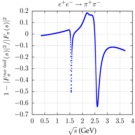
Figure 2: (color online) The relative difference between the form modulus square of the pion form factor and the form factor calculated with first six ($N=0,...,5$) resonances.

We have attempted to fit the experimental data keeping the coupling constants $c_{\rho_{n}}^{\pi}$ fixed to the model values (one fit parameter $\beta$ for all of them) and fitting only the masses and the widths of the first few resonances (up to $n=5$). This parameterization is satisfactory up to $\sqrt{s}\sim 1.3-1.4$ GeV, where the details of the model for resonances, with $n=2$ and higher, are not important. However, the model is definitively too simple for a description of the details of higher radial excitations including issues like coupled channels in decays of the higher radial $\rho$ excitations. Hence we adopt a heuristic approach, where we allow for arbitrary complex couplings $f_{n}$ of the $\rho_{n}$ ($n=1,2,3,4,5$)

$$f_{n}=F_{n}\left(\sum_{i=1}^{5}c_{\rho_{i}}^{\pi}\right)/\left({\sum_{i=1}^{5}F_{i}}\right)\,,$$ (11)

with $F_{1}=1$ and four complex constants $F_{n}\ ,\ n=2,3,4,5$ fitted to the experimental data.

The mass and the width of $\rho_{3}$ are fixed to their values obtained in the fit to the four pion production data Czyz:2008kw . For the masses and widths of the higher excitations ($n\geq 4$) we use their model values.

The results are shown in Table 1. The fitted value of $m_{\rho_{0}}$ is smaller than its PDG2008 Amsler:2008zz value, a consequence of using the dressed form factor in Akhmetshin:2003zn ; Akhmetshin:2006bx ; Akhmetshin:2006wh ; Achasov:2005rg ; Aulchenko:2006na . This phenomenon was also observed in Ghozzi:2003yn . The parameters describing the radial $\rho$ excitations obtained in the fit have to be taken with great care as they are strongly correlated, while in Table 1 we give only MINOS (MINUIT procedure from CERNLIB) parabolic errors.

To ilustrate the numerical importance of the higher radial excitations within the “dual QCD model” in Fig. 2 we show the relative difference between the full modulus square of the pion form factor and the result calculated with the first six resonances which were used in the fit. It is evident that it is impossible to neglect the higher resonances and even in the $\rho_{0}$ region they give small, but not negligible contribution to the form factor.

III The kaon form factor

The kaon form factors were revisited for the same reasons as the pion form factor. Compared to the CLEO-c result Pedlar:2005sj the model presented in Bruch underestimates the kaon form factor in the vicinity of the $\psi(2S)$ resonance. It is impossible to fit the existing data, including the CLEO-c result, with the functional form used in Bruch or adding one or two more radial excitations, unless one would accept inclusion of a huge wide resonance in the region between $J/\psi$ and $\psi(2S)$. To cure the situation, a model analogous to the one used for the pion form factor, assuming an infinite tower of resonances, was adopted. The ansatz reads

$$F_{K^{+}}(s)=\frac{1}{2}\biggl{(}\left[\sum\limits_{n=0}^{N_{\rho}}c_{\rho_{n}}^{K}BW_{\rho_{n}}(s)\right]_{fit}+\left[\sum\limits_{n=N_{\rho}+1}^{\infty}c_{\rho_{n}}^{K}BW_{\rho_{n}}(s)\right]_{dQCD}\biggr{)}$$

$$+\frac{1}{6}\biggl{(}\left[\sum\limits_{n=0}^{N_{\omega}}c_{\omega_{n}}^{K}BW_{\omega_{n}}^{c}(s)\right]_{fit}+\left[\sum\limits_{n=N_{\omega}+1}^{\infty}c_{\omega_{n}}^{K}BW^{c}_{\omega_{n}}(s)\right]_{dQCD}\biggr{)}$$

$$+\frac{1}{3}\biggl{(}\left[\sum\limits_{n=0}^{N_{\phi}}c_{\phi_{n}}^{K}BW_{\phi_{n}}^{K}(s)\right]_{fit}+\left[\sum\limits_{n=N_{\phi}+1}^{\infty}c_{\phi_{n}}^{K}BW^{K}_{\phi_{n}}(s)\right]_{dQCD}\biggr{)}\,,$$ (12)

$$F_{K^{0}}(s)=-\frac{1}{2}\biggl{(}\left[\sum\limits_{n=0}^{N_{\rho}}c_{\rho_{n}}^{K}BW_{\rho_{n}}(s)\right]_{fit}+\left[\sum\limits_{n=N_{\rho}+1}^{\infty}c_{\rho_{n}}^{K}BW_{\rho_{n}}(s)\right]_{dQCD}\biggr{)}$$

$$+\frac{1}{6}\biggl{(}\left[\sum\limits_{n=0}^{N_{\omega}}c_{\omega_{n}}^{K}BW_{\omega_{n}}^{c}(s)\right]_{fit}+\left[\sum\limits_{n=N_{\omega}+1}^{\infty}c_{\omega_{n}}^{K}BW^{c}_{\omega_{n}}(s)\right]_{dQCD}\biggr{)}$$

$$+\frac{1}{3}\biggl{(}\left[\eta_{\phi}c_{\phi_{0}}^{K}BW_{\phi_{0}}^{K}(s)+\sum\limits_{n=1}^{N_{\phi}}c_{\phi_{n}}^{K}BW^{K}_{\phi_{n}}(s)\right]_{fit}+\left[\sum\limits_{n=N_{\phi}+1}^{\infty}c_{\phi_{n}}^{K}BW^{K}_{\phi_{n}}(s)\right]_{dQCD}\biggr{)}\,.$$ (13)

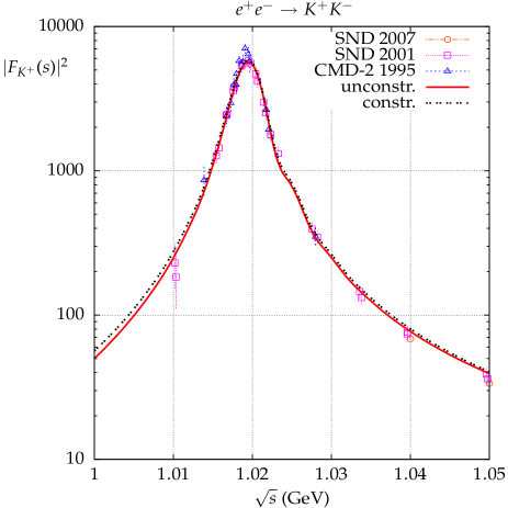
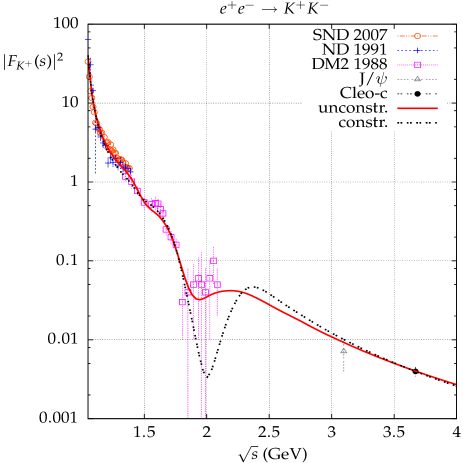
Figure 3: (color online)The experimental data Bisello:1988ez ; Dolinsky:1991vq ; Akhmetshin:1995vz ; Achasov:2001ni ; Pedlar:2005sj ; Achasov:2007kg compared to the model fits results (see text for details). The form factor at $J/\psi$ comes from its theoretical extraction Seth:Jphi from the data. It was not used in the fit.

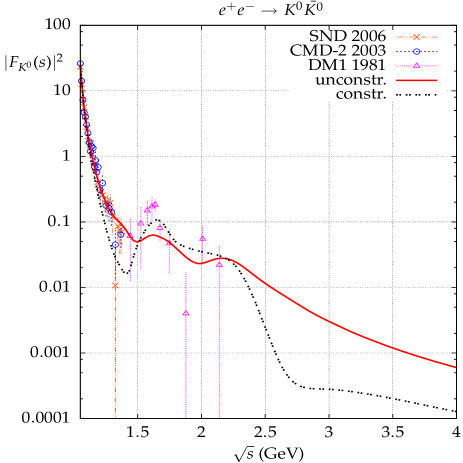
Figure 4: (color online )The experimental data Mane:1980ep ; Achasov:2001ni ; Akhmetshin:2002vj ; Akhmetshin:2003zn ; Achasov:2006bv compared to the model fits results (see text for details).

The couplings in the part with subscript $fit$ were fitted to the experimental data as well as the constants $\eta_{\phi}$ and $c_{\phi_{0}}^{K}$. The values of $N_{\rho},N_{\omega}$ and $N_{\phi}$ are listed in Table 2. The entry PDG in Table 2 implies, that masses and widths as given in PDG2008 Amsler:2008zz were used. The masses and widths of the radial excitations, which were not measured, were calculated assuming an equidistant mass spectrum and a linear relation between the mass and the width of a given resonance

$$m_{j_{n}}^{2}=m_{j}^{2}(1+2n),\,\ \Gamma_{j_{n}}=\gamma_{j}m_{j_{n}},\ \ \ j=\rho,\omega,\phi\ .$$ (14)

The value of $\gamma_{\rho}$ was calculated from Eq.(14) for $n=0$, the other values were fitted to the data.

Two versions of the model were investigated: the ‘unconstrained’ version were the couplings between kaons and $\rho_{n}$, $\omega_{n}$ and $\phi_{n}$ are not related and the ‘constrained’ version were $c_{\omega_{n}}^{K}=c_{\rho_{n}}^{K}\ ,\ n=0,\cdots\infty$. The ‘constrained’ model is not able to reproduce data as good as the ‘unconstrained’ model, however as evident from Tab. 2 the corrections to the assumption $c_{\omega_{n}}^{K}=c_{\rho_{n}}^{K}$ are small for the lowest two resonances.

Despite this, the two models predict completely different asymptotic behaviour of the neutral kaon form factor in the region, where no data are available (Fig. 4). The ‘constrained’ model, being closer to the SU(3) symmetric case where the neutral kaon form factor vanishes, arrives at significantly smaller predictions. The values of the couplings, which were not fitted, were calculated from the formula

$$c^{K}_{j_{n}}=\frac{(-1)^{n}\Gamma(\beta^{K}_{j}-1/2)}{\alpha^{\prime}\sqrt{\pi}m_{j_{n}}^{2}\Gamma(n+1)\Gamma(\beta^{K}_{j}-1-n)},$$

$$\alpha^{\prime}=1/(2m_{j_{0}}^{2}),\ \ j=\rho,\omega,\phi$$ (15)

with the exception of the couplings next to the last fitted, which were calculated from the normalization requirements

$$\sum_{n=0}^{\infty}c^{K}_{j_{n}}=1\,,\ \ \ \ \ j=\rho,\omega,\phi\,.$$ (16)

Breit-Wigner propagators

$$BW_{\alpha}^{c}=\frac{m^{2}_{\alpha}}{m^{2}_{\alpha}-s-im_{\alpha}\Gamma_{\alpha}},\ \ \alpha=\omega_{n}$$ (17)

with constant widths were used for all $\omega_{n}$, Breit-Wigner propagators with s-dependant widths

$$\kern-10.0ptBW^{j}_{\phi_{n}}=\frac{m^{2}_{\phi_{n}}}{m^{2}_{\phi_{n}}-s-im_{\phi_{n}}\Gamma_{\phi_{n}}^{j}},\$$

$$\Gamma_{\phi_{n}}^{j}=\frac{m^{2}_{\phi_{n}}}{s}\biggl{(}\frac{s-4m_{j}^{2}}{m^{2}_{\phi_{n}}-4m_{j}^{2}}\biggr{)}^{\frac{3}{2}}\Gamma_{\phi_{n}},$$

$$j=K^{+},K^{0}$$ (18)

were used for $\phi_{n}$, the radial excitations of $\phi$, and the $GS$ Breit-Wigner functions (Eq.(2)) were used for $\rho_{n}$. The parameters $\beta^{K}_{j},\ \ j=\rho,\omega,\phi$, were calculated from Eq.(15) using fitted $c^{K}_{j_{0}}$ parameter. The results of the fits are summarized in Tab. 2 and in Figs. 3 and 4. The high energy behaviour of both form factors is completely driven by the CLEO Pedlar:2005sj measurement.

Following Bruch , i.e. assuming isospin symmetry, one arrives at the following predictions for the branching ratio of the $\tau$-lepton decay into $K^{-}K^{0}\nu_{\tau}$

$$Br(\tau^{-}\to K^{-}K^{0}\nu_{\tau}) = (0.135/0.190)\cdot 10^{-3}$$ (19)

for ‘unconstrained’ and ‘constrained’ models, respectively. The model dependence is characterized by the spread between the two results and is far larger than the errors resulting from the fits of the parameters within one model. These results can be compared with the PDG value Amsler:2008zz

$$Br(\tau^{-}\to K^{-}K^{0}\nu_{\tau}) = (0.158\pm 0.16)\cdot 10^{-3}$$ (20)

and are found to be reasonably consistent.

Within the same assumptions one can predict the $K^{-}K^{0}$ invariant mass distribution and compare it (see Fig. 5) with existing CLEO data Coan:1996iu . As evident from Fig. 5 both models give very similar predictions and both agree with the data. Thus we conclude that within the current experimental accuracy, which is, however, very poor, isospin symmetry works well and the details of the models do not play any role in its tests.

Parameter	Input	Fit(1)	Fit(2)	PDG value	model(1)	model(2)
$m_{\phi_{0}}$	-	1019.415 $\pm$ 0.004	1019.415 $\pm$ 0.003	1019.455 $\pm$ 0.020	input	input
$\Gamma_{\phi_{0}}$	-	4.34 $\pm$ 0.01	4.22 $\pm$ 0.04	4.26 $\pm$ 0.05	input	input
$m_{\phi_{1}}$	1680	-	-	1680 $\pm$ 20	1766	1766
$\Gamma_{\phi_{1}}$	150	-	-	150 $\pm$ 50	353	353
$m_{\rho_{0}}$	775.49	-	-	775.49 $\pm$ 0.34	input	input
$\Gamma_{\rho_{0}}$	149.4	-	-	149.4 $\pm$ 1.0	input	input
$m_{\rho_{1}}$	1465	-	-	1465 $\pm$ 25	1345	1345
$\Gamma_{\rho_{1}}$	400	-	-	400 $\pm$ 60	259	259
$m_{\rho_{2}}$	-	1680 $\pm$ 4	PDG	1720$\,\pm$ 20	1734	1734
$\Gamma_{\rho_{2}}$	-	365 $\pm$ 59	PDG	250 $\pm$ 100	334	334
$m_{\omega_{0}}$	782.65	-	-	782.65 $\pm$ 0.12	input	input
$\Gamma_{\omega_{0}}$	8.49	-	-	8.49 $\pm$ 0.08	input	input
$m_{\omega_{1}}$	1425	-	-	1400-1450	1356	1356
$\Gamma_{\omega_{1}}$	-	145 $\pm$ 9	PDG	180-250	678	678
$m_{\omega_{2}}$	-	1729 $\pm$ 76	PDG	1670 $\pm$ 30	1750	1750
$\Gamma_{\omega_{2}}$	-	245 $\pm$ 9	PDG	315 $\pm$ 35	875	875
$\eta_{\phi}$	-	1.040 $\pm$ 0.007	1.055 $\pm$ 0.010	-	-	-
$\beta_{\phi}$	$c^{K}_{\phi_{0}}$ (15)	1.97 $\pm$ 0.02	1.91 $\pm$ 0.02	-	-	-
$\gamma_{\phi}$	-	0.2	0.2	-	input	input
$c^{K}_{\phi_{0}}$	-	0.985 $\pm$ 0.006	0.947 $\pm$ 0.009	-	input	input
$c^{K}_{\phi_{1}}$	-	0.0042 $\pm$ 0.0015	0.0136 $\pm$ 0.0024	-	0.0084	0.0271
$c^{K}_{\phi_{2}}$	-	0.0039 $\pm$  0.0026	(16)0.0214 $\pm$ 0093	-	0.0026	0.0088
$c^{K}_{\phi_{3}}$	-	(16)0.0033 $\pm$ 0.0067	-	-	0.0012	-
$\sum\limits_{n=N_{\phi}+1}^{\infty}c^{K}_{\phi_{n}}$	model	0.0036	0.0180	-	0.0036	0.0180
$\beta_{\rho}$	$c^{K}_{\rho_{0}}$ (15)	2.23 $\pm$ 0.06	2.21 $\pm$ 0.05	-	-	-
$\gamma_{\rho}$	-	0.193 (14) (= $\Gamma_{\rho}$/$m_{\rho}$)	0.193 (14) (= $\Gamma_{\rho}$/$m_{\rho}$)	-	input	input
$c_{\rho_{0}}^{K}$	-	1.138 $\pm$ 0.011	1.120 $\pm$ 0.007	-	input	input
$c_{\rho_{1}}^{K}$	-	-0.043 $\pm$ 0.014	-0.107 $\pm$ 0.010	-	-0.087	-0.078
$c_{\rho_{2}}^{K}$	-	-0.144 $\pm$ 0.015	-0.028 $\pm$ 0.012	-	-0.020	-0.019
$c_{\rho_{3}}^{K}$	-	-0.004 $\pm$ 0.007	(16)0.032 $\pm$ 0.017	-	-0.0084	-0.0079
$c_{\rho^{{}_{4}}}^{K}$	-	(16)0.0662 $\pm$ 0.0243	-	-	-0.0045	-
$\sum\limits_{n=N_{\rho}+1}^{\infty}c^{K}_{\rho_{n}}$	model	-0.0132	-0.0170	-	-0.0132	-0.0170
$\beta_{\omega}$	$c^{K}_{\omega_{0}}$ (15)	$\beta_{\rho}$	2.75 $\pm$ 0.06	-	-	-
$\gamma_{\omega}$	-	0.5	0.5	-	input	input
$c_{\omega_{0}}^{K}$	-	$c^{K}_{\rho_{0}}$	1.37 $\pm$ 0.03	-	input	input
$c_{\omega_{1}}^{K}$	-	$c^{K}_{\rho_{1}}$	-0.173 $\pm$ 0.003	-	-0.087	-0.345
$c_{\omega_{2}}^{K}$	-	$c^{K}_{\rho_{2}}$	-0.621 $\pm$ 0.020	-	-0.020	-0.026
$c_{\omega_{3}}^{K}$	-	$c^{K}_{\rho_{3}}$	(16)0.43 $\pm$ 0.04	-	-0.0084	-0.0079
$c_{\omega_{4}}^{K}$	-	$c^{K}_{\rho_{4}}$	-	-	-0.0045	-
$\sum\limits_{n=N_{\omega}+1}^{\infty}c^{K}_{\omega_{n}}$	model	$\sum\limits_{n=N_{\rho}+1}^{\infty}c^{K}_{\rho_{n}}$	-0.0096	-	-0.0132	-0.0096
$\chi^{2}/d.o.f.$	-	277/256	221/260	-	-	-

Table 2: Parameters of the kaon form factors and results of the fit to the data. Masses and widths are given in MeV. The column ’Fit(1)’ (Fit(2)) contains the values of the constrained (unconstrained) fits.

.

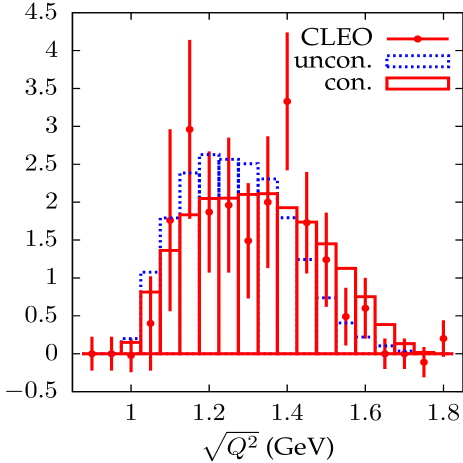
Figure 5: (color online). Normalized distributions $\frac{d\Gamma(\tau\to K^{-}K^{0}\nu_{\tau})/d\sqrt{Q^{2}}}{\Gamma(\tau\to K^{-}K^{0}\nu_{\tau})}$ of the kaon pair invariant mass predicted within two models, described in the text. CLEO data Coan:1996iu normalized to the total number of events are also shown.

IV Monte Carlo implementation of $K^{+}K^{-}$ and $K^{0}\bar{K}^{0}$

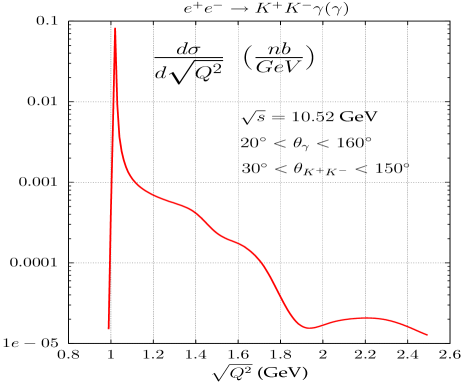
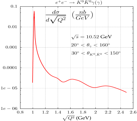
Figure 6: (color online) Differential cross section for $\sqrt{s}=10.52{\rm GeV}$ of the processes $e^{+}e^{-}\to K^{+}K^{-}\gamma(\gamma)$ and $e^{+}e^{-}\to K^{0}\bar{K}^{0}\gamma(\gamma)$ with angular cuts.

The event generator PHOKHARA has been extended to generate $K^{+}K^{-}$ and $K^{0}\bar{K}^{0}$ final states. In this section we present the implementation and results for the region below the narrow resonances $J/\psi$ and $\psi(2S)$. Charged kaons have been implemented in the same way as the $\pi^{+}\pi^{-}$ channel Czyz:2002np ; Czyz:PH03 , with the kaon form factor described in Section III. The NLO FSR corrections have been implemented as well. For the neutral kaons the corrections are limited to ISR. With the enormous luminosity of B factories one expects hundreds of events even for $Q^{2}$ between 3 and 4 $GeV^{2}$ and large statistic around the $\phi$ resonance (Fig. 6). The next-to-leading FSR corrections are relevant for a measurement in the neighbourhood of the $\phi$ resonance if an accuracy better then 10% is aimed (Fig. 7).

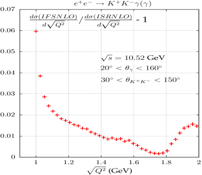
Figure 7: (color online) Comparison of IFSNLO and ISRNLO distributions with angular cuts.

V Narrow resonances and the radiative return

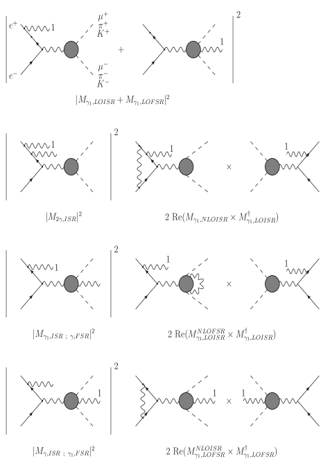
Figure 8: (color online). The contributions to the radiative return cross section included in PHOKHARA. Label ’1’ at a photon line means that the photon is hard.

The radiative return, as implemented now in PHOKHARA, receives contributions from a multitude of amplitudes shown in Fig. 8. The notation introduced in this figure also applies to the narrow resonance amplitudes. Below we list the formulae for $\mu^{+}\mu^{-}$, $\pi^{+}\pi^{-}$, $K^{+}K^{-}$ and $\bar{K}^{0}K^{0}$. For the $\bar{K}^{0}K^{0}$ amplitude $FSR$ emission is not present. We explicitly indicate the vacuum polarization contributions as well as the $\phi$ contribution. We assume that in the vacuum polarization $J/\psi$, $\psi(2S)$ and $\phi$ were not accounted for. The differential cross section given by PHOKHARA reads

$$d\sigma=$$

$$|M_{\gamma_{1},LOISR}\cdot C^{VP}_{R,P}(Q^{2})+M_{\gamma_{1},LOFSR}\cdot C^{VP}_{R,P}(s)|^{2}d\Phi_{1}$$

$$+|M_{2\gamma,ISR}\cdot C^{VP}_{R,P}(Q^{2})|^{2}d\Phi_{2}$$

$$+2\ {\rm Re}(M_{\gamma_{1},NLOISR}\times M^{\dagger}_{\gamma_{1},LOISR})\cdot|C^{VP}_{R,P}(Q^{2})|^{2}d\Phi_{1}$$

$$+|M_{\gamma_{1},ISR\ ;\ \gamma,FSR}\cdot C^{VP}_{R,P}((Q+k_{\gamma})^{2})|^{2}d\Phi_{2}$$

$$+2\ {\rm Re}(M_{\gamma_{1},LOISR}^{NLOFSR}\times M^{\dagger}_{\gamma_{1},LOISR})\cdot|C^{VP}_{R,P}(Q^{2})|^{2}d\Phi_{1}$$

$$+|M_{\gamma,ISR\ ;\ \gamma_{1},FSR}\cdot C^{VP}_{R,P}((Q+k_{\gamma_{1}})^{2})|^{2}d\Phi_{2}$$

$$+2\ {\rm Re}(M_{\gamma_{1},LOFSR}^{NLOISR}\times M^{\dagger}_{\gamma_{1},LOFSR})\cdot|C^{VP}_{R,P}(s)|^{2}d\Phi_{1}\ ,$$

where

$$C^{VP}_{R,P}(s) = \frac{1}{1-\Delta\alpha(s)}-\frac{3\Gamma_{e}^{\phi}}{\alpha m_{\phi}}\ BW_{\phi}(s)\delta_{P}$$ (22)

$$+C_{J/\psi,P}(s)+C_{\psi(2S),P}(s)\ ,$$

$$C_{R,P}(s)=\frac{3\sqrt{s}}{\alpha}\frac{\Gamma_{e}^{R}(1+c_{P}^{R})}{s-M_{R}^{2}+i\Gamma_{R}M_{R}}\ .$$ (23)

and $d\Phi_{1}$ ($d\Phi_{2}$) denote the phase space with one (two) photon(s) in the final state with all statistical factors included.

For $P=\mu$ and $P=\pi$, $c_{P}^{R}=0$ (no direct decay of the narrow resonances into $\mu^{+}\mu^{-}$ and $\pi^{+}\pi^{-}$), while $\delta_{P}=0$ for $P=K$ and $\delta_{P}=1$ for $P=\mu$ and $P=\pi$. The $\phi$ contributions to the kaon pair production are included in the kaon form factor, hence $\delta_{K}=0$. The notation and the detailed description of the narrow resonance contribution to the amplitude can be found in Czyz:2009vj (see Yuan:2003hj for similar studies). From Czyz:2009vj we also take $|c_{K^{+}}^{J/\psi}|=1.27\pm 0.32$ and $|c_{K^{+}}^{\psi(2S)}|=2.94\pm 0.99$. The information on the neutral kaon couplings to the narrow resonances is almost nonexisting and we use the lower limits of $|c_{K^{0}}^{J/\psi}|=2.81$, $|c_{K^{0}}^{\psi(2S)}|=5.35$, which correspond to the upper limit on the neutral kaon form factor (see Czyz:2009vj for details). The phases are essentially not known and we use $100^{\circ}$ to obtain the numerical values in the next section.

VI The implementation of narrow resonances into the Monte Carlo event generator PHOKHARA

The tests of the ISR part of the implementation of the narrow resonances where straightforward and followed the standard tests we perform for each new channel Rodrigo:2001kf ; Czyz:2002np ; Czyz:PH03 ; Nowak ; Czyz:PH04 ; Czyz:2004nq ; Czyz:2005as ; Czyz:2008kw . The comparisons were made with the analytic formulae of Berends:1987ab separately for one and two photon emission. The precision of the comparisons was at the level of a small fraction of a per mill, proving the technical precision of the program at that level. The independence of the results on the separation parameter between soft photon, calculated analytically and hard photon, generated by means of the Monte Carlo method, was also tested with that precision.

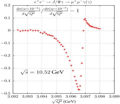
Figure 9: (color online) Comparison between invariant mass distributions obtained with $w=10^{-4}$ and $w=10^{-7}$.

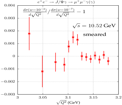
Figure 10: (color online) Comparison between invariant mass distributions obtained with $w=10^{-4}$ and $w=10^{-7}$ smeared with Gaussian with the standard deviation of 14.5 MeV.

The implementation of the NLO FSR part is more tricky. The analytic formulae used in Czyz:PH03 ; Czyz:PH04 for soft photon contributions are still valid, which we have checked numerically with the precision of 0.02%. However if one chooses the separation parameter between soft and hard part at the usual value $w=10^{-4}$, which corresponds to the photon energy $E_{\gamma}=1$ MeV for $\sqrt{s}=10$ GeV, the ‘soft’ integral receives contributions from the whole resonance region, as a consequence of the small width ( $\Gamma_{J/\psi}=93.4$ keV). For a cutoff of $10^{-4}$ the part of the matrix element, which multiplies the soft emission factor is rapidly varying and the basic assumption underlying the whole approach, that the soft emission can be integrated analytically with the multiplicative remainder being constant, is not longer valid. Pushing the value of the cutoff to an extremely small value, say $10^{-7}$, solves this problem. However, single-photon emission is not an adequate description for such soft photons and in principle one should use exponentiation. From the technical side this is reflected in the appearance of negative weights. Inclusion of YFS-like multi-photon production would allow to cure this problem. However since this would amount to completely restructuring our Monte Carlo generator, we have adopted a simpler approach, which gives correct distributions, when convoluted with an energy resolution typical for a detector at a $\phi$- or $B$-meson factory.

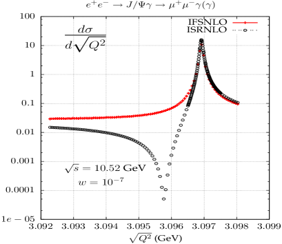
Figure 11: (color online) Comparisons of the invariant mass distributions obtained with $w=10^{-7}$ taking into account only ISRNLO contributions and the complete (ISR+FSR)NLO result.

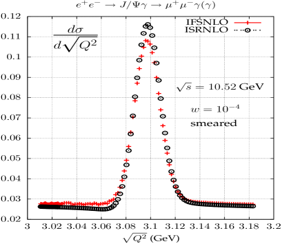
Figure 12: (color online) Comparisons of the invariant mass distributions obtained with $w=10^{-7}$ taking into account only ISRNLO contributions and the complete (ISR+FSR)NLO result. Detector smearing effect are taken into account.

Due to the finite detector resolution one never observes the true distribution of the events, but the one convoluted with the detector resolution function. This increase of the effective width by about a factor hundred is sufficient to cure the problem. For a cutoff of $10^{-4}$ the distribution remains smooth and we can produce the unweighted events sample. The result will, as expected, depend on the resolution of the detector. To check if this is true for the realistic energy resolution of the BaBar detector Aubert:2003sv of 14.5 MeV we have compared the muon invariant mass distributions obtained with $w=10^{-4}$ and $w=10^{-7}$, smeared with a Gaussian distribution with a standard deviation of 14.5 MeV. Even if the non-smeared distributions are completely different, as shown in Fig. 9 the smeared distributions agree within 2 per mill as shown in Fig. 10. This 2 per mill is the intrinsic error coming from the method we use, but the generator should be accurate enough for any practical purposes.

It is interesting to observe (Fig. 11 ) that the FSRNLO contributions fill completely the interference dip, still visible if only ISR corrections are taken into account. Thus the absence of the dip in the observed invariant mass distribution is not only the effect of the detector smearing.

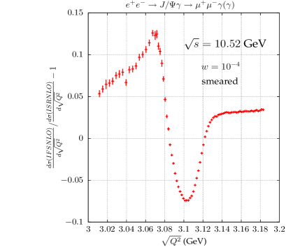
Figure 13: (color online) Relative ratio of the invariant mass distributions taking into account only ISRNLO contributions and the complete (ISR+FSR)NLO result. Detector smearing effect are taken into account.

The huge FSRNLO corrections seen in Fig. 11 are washed out if one looks at the detector smeared distributions shown in Fig. 12. The corrections are seen more accurately in Fig. 13, where the relative difference is shown. The FSRNLO corrections cannot be neglected if one aims at a precision better then 10%, unless one considers only the integral over the whole resonance region (together with the side bands as shown in Fig. 12). In the integrated cross section a large part of the corrections cancel ($\sigma_{ISRNLO}=6.901$ pb, $\sigma_{IFSRNLO}=6.954$ pb).

Identical tests were performed for the pion pair production with identical conclusions, so we do not present them here.

VII Summary

New parametrizations of the pion and kaon form factors, based on the ”dual QCD model”, are presented which are derived from a fit to a combination of old measurments and more recent experimental results in the energy region above the $\rho$-resonance. These form factors and the results of a recent analysis of the direct hadronic coupling of $K\bar{K}$ to $J/\psi$ and $\psi(2S)$ are incorporated in the Monte Carlo generator PHOKHARA which is now also adapted to the simulation of narrow resonances, including the effects of ISR and FSR in NLO.