Re-Assembling the Sagittarius Dwarf Galaxy

Abstract

What is the mass of the progenitor of the Sagittarius (Sgr) dwarf galaxy? Here, we reassemble the stellar debris using SDSS and 2MASS data to find the total luminosity and likely mass. We find that the luminosity is in the range $9.6-13.2\times 10^{7}L_{\odot}$ or $M_{V}\sim-15.1-15.5$, with $70\%$ of the light residing in the debris streams. The progenitor is somewhat fainter than the present-day Small Magellanic Cloud, and comparable in brightness to the M31 dwarf spheroidals NGC 147 and NGC 185. Using cosmologically motivated models, we estimate that the mass of Sgr’s dark matter halo prior to tidal disruption was $\sim 10^{10}M_{\odot}$.

1. Introduction

The Sagittarius (Sgr) dwarf galaxy is the closest Milky Way companion ($\sim 24$ kpc from the sun) and is currently being disrupted in the Galaxy’s tidal field. Both leading and trailing tidal streams have been detected using many different tracer populations, including A stars (Yanny et al., 2000), RR Lyraes (Vivas et al., 2001; Watkins et al., 2009), red clump stars (Mateo et al., 1998; Majewski et al., 1999) and main sequence turn-off stars (Martínez-Delgado et al., 2001; Newberg et al., 2002). Perhaps the most spectacular views of the Sgr stream are given by the M giants (Majewski et al. 2003). A portion of the stream around the North Galactic Cap has been traced to much fainter magnitudes using data from the Sloan Digital Sky Survey (SDSS, see Belokurov et al. 2006a “The Field of Streams”) revealing a prominent bifurcation into the so-called streams A and B. There has been considerable effort in modelling the disruption of Sgr since the stream stars are useful tracers for the shape of the Milky Way’s dark halo potential. Nonetheless, this work has yielded ambiguous results. Depending on which datasets are fit, oblate (Johnston et al., 2005), prolate (Helmi, 2004), spherical (Fellhauer et al., 2006), or even triaxial (Law et al., 2009) halos are preferred.

One reason for this ambiguity is that the structure, size and nature of the Sgr progenitor are very uncertain. The original luminosity and mass of Sgr is larger than its luminosity and mass today by amounts depending on the mass density (including any dark matter) and orbital history of the system. A neat illustration of this is provided by the work of Jiang & Binney (2000), who used N-body simulations to show that the current configuration of the core of Sgr can be produced by a very wide variety of initial conditions. At one extreme, the Sgr dwarf might initially possess a mass in excess of $\sim 10^{11}{{M_{\odot}}}$ and fall into the Galaxy from a distance in excess of 200 kpc. At the other extreme, it might be only $\sim 10^{9}{{M_{\odot}}}$ and start off at distances similar to its present apocenter of 60 kpc.

In this paper, we analyse the number of stars and the luminosity of the present-day Sgr core and debris. By re-assembling Sgr, we provide new constraints on its parameters prior to disruption. We describe the data sets used for this study in §2 and analyse the colour-magnitude distributions of the stream and core as well as the luminosity density along the leading and trailing arms in §3. We discuss the implications of our work for estimating the mass of Sagittarius and conclude in §4.

2. Data

We trace the Sgr stream using main sequence, red giant and horizontal branch stars from the SDSS (York et al. 2000), together with M giants in the Two Micron All-Sky Survey (2MASS). SDSS is an imaging and spectroscopic survey that covers one-quarter of the celestial sphere including an area of $\sim 8400$ deg² around the North Galactic Cap, which contains a portion of the leading arm of the Sgr stream. There are also some imaging stripes that sparsely sample low Galactic latitude fields ($\sim 3200$ deg²) which contain parts of the trailing arm. The imaging data are collected in five passbands ($u,g,r,i,z$), for which there are model isochrones (Girardi et al., 2004; Dotter et al., 2008) and photometric transformations  readily available. Here, we use positions and magnitudes of stars extracted from Data Release 7 (Abazajian et al., 2009) and corrected for extinction using the maps of Schlegel, Finkbeiner, & Davis (1998). The bright limit in the $u$-band is about 14 mag, whilst the faint limit is about 22. The final SDSS sample contains $\sim 3,740,000$ stars along the Sagittarius stream and $\sim 3,200,000$ stars in a comparison field in the North Galactic Cap region as well as $\sim 294,000$ stars along the stream and $\sim 255,000$ stars in the comparison fields in the southern stripes. We additionally use the positions and $J,H,K$ magnitudes of $\sim 1,450,000$ stars in the 2MASS All-Sky Point Source Catalog. This is complete down to roughly $K=15$ mag.

Finally, we use a dataset from Bellazzini et al. (2006) to study the properties of the Sgr core. It comprises of two fields ($\sim 299,000$ stars on and $\sim 57,000$ stars off the Sgr core) in two passbands $B$ and $V$. The sample goes approximately $3$ magnitudes below the main sequence turn-off and includes stars up to the red clump, blue horizontal branch and M giants.

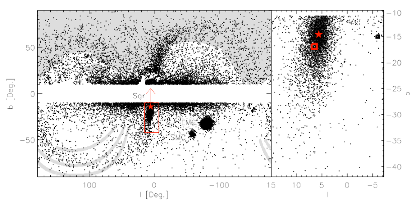
Figure 1.— Left: M giants selected from 2MASS tracing the Sgr stream in Galactic coordinates. The box marks the central parts of the Sgr dwarf and the arrow indicates the direction of motion of the dwarf. The leading and trailing arms are visible at positive and negative Galactic latitude respectively. The gray-scale shows the SDSS footprint. Right: Zoom-in of the area outlined by the box, with the fields of Bellazzini et al. (2006) marked with squares. The photometric center of Sgr is marked with a star.

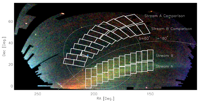
Figure 2.— “Field of Streams” (Belokurov et al., 2006a) with the Sgr debris bifurcated into a lower (A) and an higher (B) declination stream. Selection boxes along the stream (used in §3.3) are shown, together with comparison boxes at the same Galactic latitude but reversing the sign in longitude, (i.e., effectively reflecting the boxes in $\ell=180^{\circ}$). The stream boxes are $5^{\circ}$ wide in right ascension and are chosen to cover the entire width of the stream in declination.

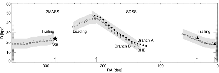
Figure 3.— Upper: Density of SDSS BHBs in the plane of distance versus right ascension for the Sgr stream (left), comparison field (middle) and their difference (right). Note the prominent linear feature associated with streams A and B, which is shadowed by the blue stragglers some 2 magnitudes fainter.The solid lines bracket the distance gradient in Sgr’s BHBs. Lower: Comparison of distances to the Sgr stream in 2MASS (open symbols) and SDSS (filled symbols, from Belokurov et al. 2006) datasets with the uncertainty in distance shown in gray. The leading arm is marked with circles, the trailing with triangles. Note the good match between distances derived from different indicators. Arrows mark locations of data-set overlaps.

3. All-Sky Views of the Sgr Stream

We begin by giving an overview of different observations of Sgr and the terminology that we will employ throughout the paper. We refer to the still bound portion of the dwarf as the core or remnant, which we define as stars within 10 kpc of the center. These stars follow a King profile (see e.g., Majewski et al. 2003). The luminosity of Sgr is usually quoted as the light integrated inside this radius, but it is not obvious that all of these stars are still gravitationally bound. The tidal debris from the disruption wraps around the Galaxy (possibly multiple times) in what is usually referred to as the leading and trailing tidal streams or arms. The portion of the debris that is seen around the North Galactic Cap is bifurcated into stream A and stream B. The working hypothesis for this paper is that both stream A and stream B are part of the leading arm. Part of the leading arm is also detected in the 2MASS survey. The trailing arm is in part covered by the southern stripes of the SDSS and more fully covered in 2MASS.

The best panorama of the Sgr stream is given by M giants selected from 2MASS, as first realized by Majewski et al. (2003). Their choice of cuts on $J,H,K$ magnitudes picks out bright red stars at the typical distances of Sgr. For Figure 1, and in the following analysis, we adopt the selection criteria introduced by Majewski et al. (2003), namely

$$J-K>0.85$$

$$J-H<0.561(J-K)+0.36$$

$$J-H>0.561(J-K)+0.22$$ (1)

$$|b|>10^{\circ}$$

$$E(B-V)<0.555$$

Additionally, for the left panel of Figure 1 only, we remove some of the reddest stars with $J-K>1.25$ and limit the magnitude (heliocentric distance) range to $10<K<12$ ($7<D<70$ kpc) for the trailing arm and to $11<K<13$ ($5<D<110$ kpc) for the leading arm. This is in order to isolate the tidal debris of the Sgr. Notice too that the Magellanic Clouds are very prominent. Superficially, Sgr already looks to be intermediate between the Large and Small Cloud in size and luminosity.

The right panel of Figure 1 shows a zoom-in of the Sgr core, made using the cuts of eqn (3), together with an additional color-magnitude (CMD) box. This is derived by shifting the ridgeline of Sgr M giants ($K=-8.650(J-K)+20.374$, Equation 5 of Majewski et al. 2003) by $\pm 3.5\sigma$ or $\pm 1.26$ mag in the color range $0.95<J-K<1.1$. Using this selection gives a clear view of the Sgr core, the photometric center of which is marked. Also shown are the on-core and off-core fields of Bellazzini et al. (2006).

The SDSS view of the Sgr stream is confined primarily to the North Galactic Cap and hence is shown in equatorial coordinates in Figure 2 to minimize distortion. The “Field of Streams” (Belokurov et al., 2006a) shows the Sgr stream over a 100^∘ arc, with an unprecedented level of detail. The datasets provided by 2MASS and SDSS are complementary – the 2MASS survey picks up the trailing arms with good clarity, but it loses the leading arm around the North Galactic Cap.

3.1. Distances

There is information about the distances to debris at a number of points along the stream  (Belokurov et al., 2006a; Newberg et al., 2007; Watkins et al., 2009). Heliocentric distances to the trailing arm were originally computed by Majewski et al. (2003), who showed that there was little distance gradient along this part of the stream. There has been more controversy about distances to the leading arm, mainly because there are much steeper distance gradients.

Given the crucial role that distances play, we begin by seeking independent confirmation of earlier results. For the leading arm in the Field of Streams, we select blue horizontal branch (BHB) candidates from the SDSS in the on and off-stream fields using the criteria given in Figure 10 of Yanny et al. (2000). This gives us $\sim 18700$ candidates in the Sgr stream and $\sim 8500$ candidates in the comparison field. We note that these numbers do not include all genuine BHBs, and suffer from some contamination from blue stragglers (BS). The upper panels of Figure 3 show the density of BHBs in the two fields, together with their difference. The distances to BHBs are calculated assuming an absolute magnitude of $M_{g}=0.7$, which is appropriate for our color range ($u-g>0.9$, see Table 2 of Sirko et al. (2004)). Running diagonally across the plot is the signal from the BHBs in the Sgr stream. It is accompanied by a fuzzy shadow of BSs two magnitudes fainter. The Galactic halo foreground appears to be slightly asymmetric, most likely due to the presence of the Virgo Overdensity (Jurić et al., 2008) in parts of the stream field. However, the subtraction works well and leaves the Sgr stream clearly visible. The stream signal is roughly linear in the plane of distance versus right ascension and can be described by a straight line with gradient 0.386. The solid lines in the two leftmost panels show the straight line fit offset by $\pm 5$ kpc. The lower panel compares the BHB distances (straight line) to the leading arm with those originally inferred by Belokurov et al. (2006a) using the $i$ magnitude of the subgiant branch in the “Field of Streams”. It is reassuring that there is excellent agreement between the two independently calculated distances, especially as the BHB’s luminosity is almost independent of age and metallicity.

Also shown are the distances to 2MASS M giants in both leading and trailing arms. Using the cuts described above, we create a density distribution of M giant stars in Sgr’s orbital plane as shown in Figure 4. Distances to pixels with highest density along the stream are then computed with a typical uncertainty of 6 kpc. This is a combination of the uncertainty in the color-absolute magnitude relation for M giants and the intrinsic width of the stream. Finally, we also show two detections of the trailing debris in the SDSS southern stripes. The distances are computed using both BHBs and main-sequence turn-off stars. The overlaps of the SDSS and 2MASS datasets will play an important role in what follows.

As a useful summary of the data, we list distances and right ascensions in Table 1. Recently, Yanny et al. (2009) reviewed the detections of the Sgr stream in SDSS data, and their results are in good agreement with ours.

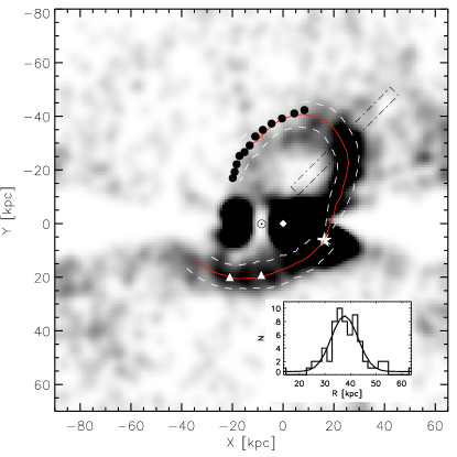
Figure 4.— Density distribution of 2MASS M giants in the orbital plane of Sgr as defined in Majewski et al. (2003, see Figure 11). The center of Sgr is marked with a star. The solid red line marks the ridge line, whilst the dashed lines indicate the $3\sigma$ boundary of the tidal arms. The circles are the SDSS observations around the North Galactic Cap. The triangles mark the stream detections in the SDSS southern stripes. The inset shows the number of M giants as a function of heliocentric distance in the dot-dashed slice of the stream. A Gaussian fit to the distribution yields a width of $6$ kpc. The Galactic Center and the Sun positions are marked.

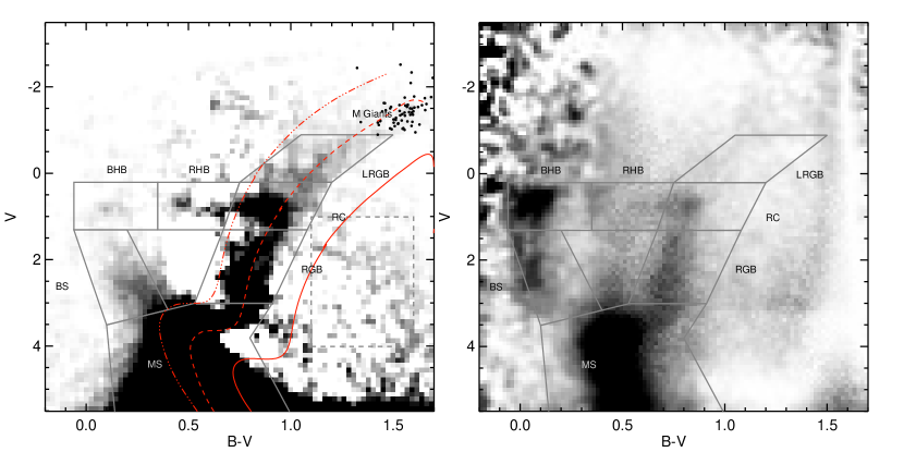
Figure 5.— Comparison of the Hess diagrams of the Sgr core (left) and stream (right). Note that the populations in the core and the stream are very similar. Boxes are overlaid to identify characteristic populations used later in the paper, including main sequence (MS), red giant branch (RGB), red clump (RC), red horizontal branch (RHB), blue horizontal branch (BHB), blue stragglers (BS), and luminous red giant branch (LRGB). The black points in the left hand panel are M giant stars selected in the core using the cuts described above. The dashed box shown in the left panel is used to scale up the density in the control field. Overplotted in the left panel are Dartmouth isochrones  (Dotter et al., 2008) of varying age and metallicity (solid $15$ Gyr, [Fe/H]$=0.0$; dashed $11$ Gyr, [Fe/H]=$-0.5$; dash-dotted $8$ Gyr, [Fe/H]$=-1.0$). We are confident that there are no turn-offs of older stellar populations in the Sagittarius core that were not detected in the Bellazzini et al. data.

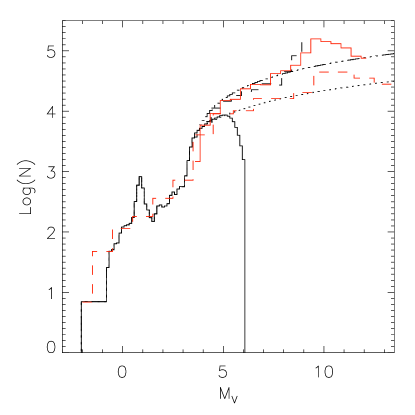
Figure 6.— LF of the Sgr remnant (black), together with two possible extrapolations at the faint end (dashed and dotted). Also shown are the LFs of Ursa Minor (black dashed), the globular cluster M15 (red solid), together with a mean globular cluster LF (red dashed).

Table 1Heliocentric Distances to parts of the Sgr stream. SDSS and 2MASS observations are summarized in the top and bottom halves respectively.

RA - Stream A	215	210	205	200	195	190	185	180	175	170	165	160	155	150	145	140	135	130	125
Distance (kpc)	47	47	46	43	40	38	35	33	30	28	27	25	24	21	20	19	18	17	16
RA - Stream B	215	210	205	200	195	190	185	180	175	170	165	160	155	150	145
Distance (kpc)	45	44	45	41	38	35	32	30	28	26	26	23	22	19	16
RA - Trailing	5	35
Distance (kpc)	19	25
RA - Leading	252	246	240	234	229	223	217	212
Distance (kpc)	36	38	40	41	43	44	44	44
RA - Trailing	286	292	298	…	316	322	328	333	…	18	22	27	31	35	39	44	48	52	57	61
Distance (kpc)	24	23	22	…	21	21	20	19	…	20	20	21	22	23	24	25	26	27	28	29

Table 2Single exponential fits to the A (top half) and B (bottom half) streams (see Figure 7). The left column gives the slope of the exponential together with its uncertainty. The middle column gives the luminosity per kpc of the fits at RA$=220^{\circ}$. The right column indicates the number of data points used in the exponential fit. Where applicable the values in brackets indicate the parameters derived using all data points.

Sample	Exponent ($\times 10^{-3}$)	Luminosity ($L_{\odot}\times 10^{4}$)	Data Points
Total	7.0 $\pm$ 0.2	27.00	12
MS	6.6 $\pm$ 0.3	15.92	12
BS	4.5 $\pm$ 0.8	0.24	12
RGB	6.4 $\pm$ 0.5	2.01	12
RC	7.7 (3.5)$\pm$ 1.0 (0.4)	2.14 (1.66)	6
RHB	8.1 $\pm$ 0.6	3.18	12
BHB	6.2 $\pm$ 1.0	0.33	12
LRGB	8.7 (-2.7)$\pm$ 0.7 (0.5)	2.12 (1.1)	4
Total	4.5 $\pm$ 0.6	15.01	12
MS	4.9 $\pm$ 0.6	9.20	12
BS	2.7 $\pm$ 0.7	0.18	12
RGB	4.1 $\pm$ 0.7	1.47	12
RC	4.4 (0.5) $\pm$ 1.2 (0.4)	1.2 (0.92)	0
RHB	5.1 $\pm$ 1.0	1.47	12
BHB	4.5 $\pm$ 1.2	0.24	12
LRGB	4.4 (-1.0) $\pm$ 1.2 (0.5)	1.2 (1.2)	0

3.2. Sagittarius Core

In order to derive the luminosity of Sgr, we need to disentangle its stars from the Galactic fore and background. We start by re-visiting the calculation of the luminosity of the remnant. The original value of Ibata et al. (1995) is based on data from Schmidt photographic plates. With an estimate of the extent of the remnant, together with a CMD of a $2.5^{\circ}\times 2.5^{\circ}$ central field, they calculated an absolute magnitude of $M_{V}\sim-13$. This relies on the similarity of the CMDs of Sgr on the one hand and Fornax and the SMC on the other. Mateo et al. (1998) acquired data on 24 fields of size $0.25^{\circ}\times 0.25^{\circ}$ across the face of Sgr and built a number density profile of main sequence stars. Then, using a surface brightness normalization from  Mateo et al. (1995), this can be integrated to give a total luminosity of the remnant as $M_{V}=-13.3$. However, due to the size of the field of view ($0.25^{\circ}\times 0.25^{\circ}$) in  Mateo et al. (1995), the luminosity function (LF) does not extend brighter than the red clump and does not include BHBs and BSs. So, the shape of the surface brightness profile is well-constrained, as confirmed by Majewski et al. (2003), but the overall normalization is more uncertain.

The data of Bellazzini et al. (2006) cover a larger area than those of Mateo et al. (1995) at the same location, and hence give a clearer view of all the stellar populations. The core data are obtained in a $1^{\circ}\times 1^{\circ}$ field approximately $2^{\circ}$ east of the Sgr center located at $(l,b)\approx(6.5^{\circ},-16.5^{\circ})$ and along the major axis. The control field is $0.5^{\circ}\times 0.5^{\circ}$ at $(l,b)\approx(-6.0^{\circ}\times-14.5^{\circ})$. For both fields, we fix the reddening at $E(B-V)=0.11$, which is the mean value over the core field, as judged from the maps of Schlegel, Finkbeiner, & Davis (1998). The left panel of Figure 5 shows the CMD of the Sgr core. This is a Hess difference that has been constructed by subtracting from the core Hess diagram the control field Hess diagram. To scale the control field density, we minimize the residual counts in the dashed box shown in Figure 5. There are a number of readily identifiable populations in the CMD, including the main sequence (MS), red giant branch (RGB), red clump (RC), red horizontal branch (RHB), blue horizontal branch (BHB), blue stragglers (BS) and the luminous red giant branch (LRGB), together with M Giants selected in the same manner as in the right-hand panel of Figure 1. We use the CMD boxes shown to build the LF of the core and calculate luminosity density profiles along the stream. It is reassuring that our core CMD looks very similar to Figure 1 of Bellazzini et al. (2006), which has been constructed from the same data, but with a different algorithm.

Figure 6 shows the observed LF of the Sgr remnant as derived from integrating the light in the CMD boxes. This drops dramatically beyond $M_{V}\sim 5$, and a number of possible extrapolations at the faint end are shown. However, most of the luminosity is in stars brighter than the turn-off. Mateo et al. (1995) computed the luminosity of the Sgr remnant by integrating the LF between the red clump and the upper-main sequence to get a surface brightness of 25.8 mag arcsec^-2. They account for the missing flux in fainter stars by extrapolating their LF to $M_{V}=13.2$ to get $0.5$ mag correction. They do not explicitly account for stars brighter than the red clump or bluer than the main-sequence turn-off. Repeating the calculation for our LF derived using the Bellazzini et al. (2006) data, we get a similar surface brightness in stars between the red clump and the upper main sequence, namely $25.7$ mag arcsec^-2. However, we also find the BHBs, BSs, LRGBs and M giants contribute an additional $0.3$ mag. Two possible extrapolations at the faint end are shown, which contribute $0.5$ mag (dot-dashed) and $0.15$ (dotted) respectively. This can be compared to LFs of a typical globular cluster (red dashed, Cox 1999), the dSph Ursa Minor (black dashed, Wyse et al. 2002) and one of the most luminous globular clusters, M15 (red solid, Piotto et al. 1997). Taking our lead from the dSph LF suggests adding $0.5$ mag for faint stars to arrive at a surface brightness of $24.9$ mag arcsec^-2 (compared to a value of $25.3$ given in Mateo et al. 1995).

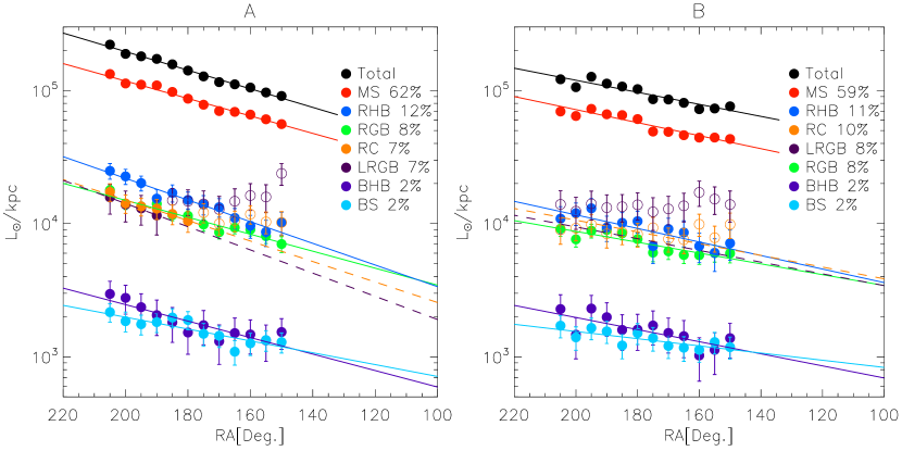
Figure 7.— Left and right panels show the luminosity per unit length in a variety of stellar populations in streams A and B respectively. The luminosities for the RGB, RC, RHB, BHB, BS and LRGB stars are derived directly from the Hess difference diagrams. The numbers are normalized to $1$ kpc distance along the stream. The luminosities in the MS stars are corrected for missing flux using the derived LF. Error bars are determined assuming Poisson noise. A single exponential is fit to each population. However, the RC and LRGB populations show significant noise and hence for stream A only the first few data points follow an exponential fit. In stream B the noise dominates these two populations and the exponential shown is estimated without using any data points as described in the main text. The fits to these two populations are therefore shown as dashed lines. The data points used in determining the fits are shown as filled symbols and those excluded as open symbols. The behavior of streams A and B is very similar, suggesting that both A and B may be parts of the same leading arm. Finally, we list at the side of the figure the mean of the fractional contribution to the total luminosity across the stream for each population.

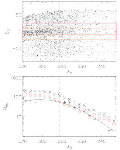
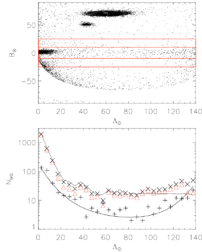
Figure 8.— Top: Location of 2MASS M giants in the orbital plane defined by the Sgr orbit; see equation 9 of Majewski et al. (2003) for the definition of latitude and longitude ($B_{\odot}$,$\Lambda_{\odot}$). The red box encloses the Sgr leading (left) and trailing (right) streams, whilst the foreground box is chosen to have the same area. Bottom: Number counts ($N_{\rm MG}$) of M giants in the stream in bins of $5^{\circ}\times 20^{\circ}$ as a function of longitude in the orbital plane. Crosses (pluses) are counts in the central (foreground) boxes. The curves are estimates of the underlying smooth foreground. The red circles and triangles are the resulting profiles. The profile of the trailing arm derived by Majewski et al. (2003) is plotted in grey in the bottom right panel.

3.3. The Density Profile of the Sagittarius Stream

The CMD of streams A and B of the Sgr leading arm is already shown in Figure 4 of Belokurov et al. (2006a) and is known to look similar to that of the core. Here, we refine the calculation of the leading arm CMD in three ways. First, we use the latest data release DR7 of the SDSS (Abazajian et al., 2009). Second, we use a different comparison field, defined by reflecting the boundaries of the stream across the $\ell=180^{\circ}$ line (see Figure 2). This assumes that the Galactic field star population is symmetric across $\ell=180^{\circ}$ and that the control fields therefore probe a similar field star population as is present around the Sgr stream. Third, in order to combine portions of the stream at different distances, we offset each star in the stream and control field using a smooth mapping between its right ascension and distance (see Figure 3). Rather than showing the difference of two Hess diagrams, here we choose to show the ratio. The advantage of this is that it accounts naturally for the fact that the depth of the CMD varies along the stream. This procedure helps to enhance fainter features like the horizontal branch and luminous part of the red giant branch, as can be seen in the right panel of Figure 5. This also explains the differences in relative density between the two panels. There are some small but significant differences in the location of CMD features. For example, the stream’s CMD is slightly bluer than the core’s. This could be due to metallicity gradients, although the bulk of it is probably due to slight underestimation of extinction in the core (which is of course very difficult to measure in low latitude fields). Nonetheless, the size of our CMD boxes means that regardless of the slight color mismatch, Sgr member stars will still be selected.

We count the numbers of stream stars in the population boxes marked in Figure 5, and subtract the counts in the comparison field. Given the distance to each field, this produces a Hess difference in absolute magnitude versus color, $M_{V}$ versus $B-V$. Due to the substantial distance gradient along the stream, the faintest population box – main sequence stars – is probed to different limiting magnitudes. To correct this, we make use of the fact that the stream’s population is similar to that of the Sgr core, at least below the subgiant branch. We extend each field’s LF down to $M_{V}=13.2$ by requiring that the slope of the stream’s LF at $M_{V}=3.4$ matches that of the core’s extrapolated LF. This value is chosen as it corresponds to the limiting SDSS magnitude $V\sim 22$ in the most distant leading arm field.

The Hess difference is integrated over each CMD box to give the total luminosity. Since each field has the same angular extent but is at a different heliocentric distance, the luminosity is normalized by the length of the segment in kpc. The two panels of Figure 7 show the luminosity profiles as a function of right ascension for multiple populations in streams A and B, together with exponential fits. The choice of fitting law is motivated by the behavior of the total luminosity. We expect that all stellar populations behave in a similar way, and this is largely confirmed by our results. There are populations not so well described by an exponential law, but these deviations may be caused by noise in the data. Each of our fields probes at least some way down the main-sequence, so the only population that is affected by our LF correction is the main-sequence sample itself. However, as shown in Figure 7, the RGB, RHB, BHB and BSs all have slopes that match the slope in the corrected main sequence sample, which suggests that the observed trend is not due to the correction we apply. Notice that the slopes of all the stellar populations in both streams A and B are positive at a statistically significant level. This implies that the corresponding densities of the populations are all fading with decreasing right ascension, that is increasing distance from the progenitor (as also noticed by Yanny et al. 2009). This is consistent with both A and B being part of the same leading stream.

Stream A is roughly a factor two brighter in luminosity than B. About $60\%$ ($50\%$) of the signal is contributed by the main sequence stars when the dot-dashed (dotted) extrapolation of Figure 6 is used. The total luminosities in the fields are on average a factor of $1.3$ brighter when using the steeper extrapolation. BHBs and BSs contribute little to the total luminosity, but can be very cleanly selected and so give a good indication of the underlying trend. By contrast, the counts corresponding to the RC and LRGB stars are much noisier. This is because the foreground contamination by the thick disc and halo is most severe, and varies considerably in the bright part of the CMD. In fact, the exponential fall-off is only present in the first few bins of stream A, corresponding to right ascensions between $180^{\circ}$ and $205^{\circ}$. The dashed lines for stream A therefore show exponential fits using only the data at higher right ascension (shown as filled symbols). For the fainter and therefore even noisier stream B, even this option is unavailable and so we assume a constant ratio of BHBs to RCs and LRGBs in the two streams to derive the dashed lines in the right-hand panel. This assumes that streams A and B have similar metallicities, which is supported by the work of Yanny et al. (2009). Table 2 gives the slope of each exponential fit together with its uncertainty, as well as the luminosity for each component at a right ascension of $220^{\circ}$. We also indicate the number of data points used in determining the exponential fit

To obtain as complete a profile of the stream as possible, we will need to exploit the complementarity of the 2MASS and SDSS datasets. 2MASS provides a powerful probe of the trailing arm, for which Majewski et al. (2003) have already deduced a profile. There are also parts of the leading arm in 2MASS, for which we build the profile as illustrated in Figure 8. The upper panel shows the locations of M giants, selected using the same method as the zoom-in of Figure 1 after offsetting stars to the distance of the core using Table 1. The results are shown in the heliocentric coordinate system aligned with the Sgr orbital plane, as defined by equation 9 of Majewski et al. (2003). There are two selection boxes in red to pick out the stream signal and the foreground. The resulting profiles of the raw number counts in $5^{\circ}$ bins, the foreground and the corrected number counts are shown in the lower panel. Applying the same procedure to M giants in the trailing arm, we recover a profile similar to that of Majewski et al. (2003), although rising in the outer parts.

Before we can begin reassembly, we need to do three more things. First, we measure distance along the stream from the progenitor to the observed fields using Table 1. Secondly, we combine streams A and B in the SDSS dataset into a single profile of the leading arm. Thirdly, in order to combine SDSS and 2MASS observations, we convert M giant number counts into total luminosity densities along the stream. We measure the relationship between the number of M giants ($N_{\rm MG}$) and the total luminosity at the locations where the Bellazzini et al. (2006) and SDSS observations overlap with the 2MASS coverage (see the lower panel of Figure 3). Here we can measure the total luminosity using the Hess difference method and count 2MASS M giants. The uncertainty in the ratio of the two is determined assuming Poisson statistics. There are clearly substantial gradients between the remnant and both the leading and trailing arms. This is illustrated in Figure 9. We use a straight line fit, which has a gradient of $280\pm 30{L_{\odot}}$ kpc^-1 per M giant. Alternatively, assuming a step function constant in the remnant and constant in the stream does not affect the following analysis substantially.

Figure 10 shows the resulting luminosity profile as a function of distance along the stream for both the leading (circles) and trailing (triangles) arms. Points derived from 2MASS data are represented by open symbols, whereas those from SDSS by filled symbols. The profiles of the leading and trailing arms are different by a factor of $\sim 3$ at small distances from the remnant, primarily as a consequence of the fact that the trailing arm is much more extended. Notice too the bump in the leading arm at $\sim 40$ kpc distance along the stream. Such features are common in simulations – such as in Figure 1 of Law et al. (2005) – as a consequence of the pile-up of material stripped at disk-crossings. There is also an evident break in the profile of the trailing arm at $\sim 10$ kpc distance along the stream, similar to that seen by Majewski et al. (2003). It is natural to associate this break with the transition between the core and the streams. Even though the profiles have a complex structure, it is useful to give a simple fit. For the trailing arm, we fit a broken exponential and find indices $-0.207$ and $0.008$ either side of a break radius at $9.6$ kpc. For the leading arm, the break radius lies behind the disk and we only measure the profile after the break as $-0.007$.

3.4. The Luminosity of Sgr

Now we begin the reassembly by calculating the total luminosity in the Sgr remnant and tidal debris. We estimate the remnant’s luminosity by summing the observations of the trailing arm within the profile break to get $2.0\pm 0.3\times 10^{7}L_{\odot}$. This is doubled on the assumption of the symmetric structure of the remnant, giving us a total magnitude of $M_{V}=-14.2\pm 0.1$, which is within 2 $\sigma$ of the value of Mateo et al. (1998) of $M_{V}=-13.4\pm 0.5$.

For the debris, we give two estimates. The first is a lower limit set by the data alone, namely $2.6\pm 0.1\times 10^{7}L_{\odot}$ for the leading arm and $8.2\pm 0.7\times 10^{6}L_{\odot}$ for the trailing. The combined value already contains more than half the core’s luminosity, and is well constrained by the deep SDSS coverage of the leading arm.

The second is an estimate of the luminosity contained within the entire debris stream, not simply the portions we observe. This is based on integrating the leading arm profile from $25$ kpc (corresponding to the first 2MASS observation) to $300$ kpc, which is triple the length to the last SDSS observation. This corresponds to a full wrap, as judged by the simulations (see e.g., Law et al., 2005; Fellhauer et al., 2006). This gives a luminosity of $3.5\pm 0.1\times 10^{7}L_{\odot}$. This nominal error is so small because the fit is constrained by the SDSS observations which have small uncertainties due to the large number of stars in the SDSS sample. This also ensures that potentially larger photometric errors on individual stars are averaged out. To account for the region between the core and $25$ kpc, we average two possible extreme cases. If we assume that the core is symmetric, then the leading arm profile needs to dip down sharply to meet the trailing arm profile at $10$ kpc. This would contribute $0.6\times 10^{7}L_{\odot}$ to the luminosity of the leading arm. Alternatively, since we do not actually observe any indication of such a dip, the profile may continue rising until joining up with the core’s profile at approximately $5$ kpc. This would contribute $1.6\times 10^{7}L_{\odot}$. Therefore, for the missing inner portion of the leading arm, we take as a compromise the average value $1.1\pm 0.5\times 10^{7}L_{\odot}$ where the large uncertainty reflects the range of possible values. The total leading arm luminosity (given by adding the extrapolated exponential and the estimate for the region between the core and the first observations)is then doubled to account for the trailing arm. We do not integrate the profile of the trailing arm since it is rising, which most likely reflects its approach to appocenter. Integrating a rising profile is obviously very sensitive to the limits of integration. At present it is difficult to make a reasonable assumption about the behavior of the trailing arm far from the core. This finally gives for the total debris luminosity $9.2\pm 0.7\times 10^{7}L_{\odot}$. This will be reduced to $6.6\pm 0.7\times 10^{7}L_{\odot}$ if the fainter LF in Figure 6 is used. It is evident that the formal error from Poisson noise, typically of order of $10\%$, is much smaller than uncertainties induced by extrapolations. To account for the missing data, we were forced to extrapolate both the luminosity function and parts of the density profiles.

The various luminosities used in the final answer are summarized in Table 3. The total luminosity of Sgr progenitor is $13.2\times 10^{7}L_{\odot}$ or $M_{V}\sim-15.5$ with the brighter LF. If we repeat the above calculation with the fainter LF, we arrive at $9.6\times 10^{7}L_{\odot}$ or $M_{V}\sim-15.1$. This implies that the progenitor is fainter than the SMC, but comparable to the brighter M31 dSphs like NGC 147 ($L=9.4\pm 2.0\times 10^{7}L_{\odot}$,$M_{V}=-15.1$) and NGC 185 ($L=13.5\pm 2.0\times 10^{7}L_{\odot}$, $M_{V}=-15.5$).

The systematic uncertainties clearly outweigh the Poisson noise but we are confident that we have atleast found a firm lower limit ($9.6\times 10^{7}L_{\odot}$) to the luminosity. The sources of systematic uncertainty include the interpolation of the inner slope of the leading arm. This is over quite a modest range and unlikely to be seriously in error. In addition considerable uncertainty derives from the extrapolation of the LF as shown above. Perhaps the greatest unknown is the behavior of the profiles at large distances. We have assumed that the exponential behavior continues to 300 kpc, but there may be processes that cause additional clumps and bumps.

Table 3Luminosity of various parts of the Sgr stream together with their associated Poisson uncertainties.

	Luminosity (in $10^{7}L_{\odot}$)
Stream Portion	Faint LF	Bright LF
Core (Bellazzini et al.)	$2\times 1.5\pm 0.3$	$2\times 2.0\pm 0.3$
Leading Arm (SDSS)	$2.0\pm 0.1$	$2.6\pm 0.1$
Trailing Arm (2MASS)	$0.6\pm 0.1$	$0.8\pm 0.1$
Leading Arm (25 to 300 kpc)	$2.5\pm 0.1$	$3.5\pm 0.1$
Leading Arm (Core to 25 kpc)	$0.8\pm 0.5$	$1.1\pm 0.5$

Figure 9.— Conversion factor between total luminosity and numbers of M giants at different locations along the stream. The dash-dotted line shows the change in the conversion factor along the stream assuming that it is constant within the core, and constant along the stream. The dashed line shows the conversion factor assuming it varies linearly throughout the core and stream.

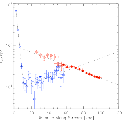
Figure 10.— Comparison between the leading and trailing arms as seen in 2MASS and SDSS. We plot here the total luminosity per unit kpc along the stream versus the distance along the stream. For the 2MASS data, this is obtained from the number counts of M giants by the scaling described in the main text. The symbols have the same meaning as in the lower panel of Figure 3. For the trailing stream, the dashed line shows the best broken exponential fit to the data. For the leading stream, the slope of the inner part is fixed which determines the break point.

4. Discussion and Conclusions

Using SDSS and 2MASS data, we have provided for the first time the luminosity profiles of both the leading and trailing arms of the Sgr stream. Prior to this work, the only available profile was that of the trailing arm derived from M giants by Majewski et al. (2003). This was essentially flat, and so cannot be extrapolated to derive useful constraints on the mass lost during disruption. Here, our profiles for both the leading and trailing arms have gradients. It is the gradient in the leading arm that enables us to derive useful constraints.

The luminosity in the leading stream clearly declines with increasing distance from the progenitor. Although the beginning of the tail is absent because it lies behind the disk, the profile still shows mild evidence for a bump. This is most likely a pile-up at apogalacticon. The trailing stream can be traced all the way from the remnant to the anti-Center, and shows a clear break around the tidal radius as we move from the core to the tail. At first glance, this looks very different to the leading arm profile. But in reality it may just be a stretched-out version of the leading profile, as the trailing arm extends to much greater Galactocentric distances. In this picture, the rising part of the profile is interpreted as the approach to an apogalacticon pile-up. We speculate that a similar but steeper rise would be observed in the leading arm, making the core profile symmetric, were it not obscured by the disk.

It is worth emphasizing that a firm lower limit $M_{V}\sim-15$ for the Sgr progenitor luminosity is given by the data with minimal assumptions. The most important is that the mass is equally apportioned between leading and trailing in both the remnant and the tails. Thanks to deep and wide SDSS coverage, the leading profile is measured with excellent accuracy. It is the tightness of the datapoints in the leading arm that is providing this firm lower limit. For example, integrating the exponential profile out to $200$ or $300$ kpc makes little difference to the final answer.

Our results may have implications for the scenario proposed by Fellhauer et al. (2006), who argued that stream A is material in the leading arm that was stripped recently, whereas stream B is debris in the trailing arm that was stripped long ago. Here, we have explicitly assumed that streams A and B are both parts of the same leading arm. This is supported by recent findings of Yanny et al. (2009), who noted that the stars in streams A and B have very similar metallicities and velocities. Also, if stream B is old and trailing, then its density (about one half of A) is larger than the young trailing arm (about a third of A), which seems counter-intuitive. So, although Fellhauer et al’s (2006) interpretation has not been ruled out, there are possible causes for concern.

The luminosity profiles offer a new, and largely unexplored, constraint on the disruption process. The fact that the leading arm profile is not flat, but decreases, directly limits the stellar mass lost in the disruption. The relative numbers of counts in the leading and trailing arms can be used to constrain the geometry of the orbit. The stars move along the tail with a drift velocity determined by the properties of the progenitor and the orbit (Dehnen et al., 2004). Therefore, the time of onset of destruction of the stellar component is in principle recoverable.

Our estimate of the progenitor luminosity is $9.6-13.2\times 10^{7}L_{\odot}$ or $M_{V}\sim-15.1--15.5$ with roughly $70\%$ of the light in the tidal tails. The nearest look-alikes in the Local Group are probably the M31 satellites NGC 147 and NGC 185. These two dSphs bracket properties of Sgr in terms of number of globular clusters, metallicity, gas content and velocity dispersion (see e.g. Tables 12.4 and 12.6 of van den Bergh, 2000). Their mass-to-light ratios are comparatively modest at $\sim 5$ (Geha et al., 2009). If we accept the comparison, then this suggests that the mass within the luminous radius of the Sgr progenitor was $\sim 10^{9}{M_{\odot}}$. This is right at the lower mass end of the range of models considered by Jiang & Binney (2000) who investigated the range of progenitor properties which could reproduce the structure of the core remnant observed today.

We can use the estimate that $70\%$ of Sgr’s luminosity now resides in the tidal debris to draw conclusions about the properties of the progenitor’s dark matter halo. Peñarrubia et al. ($2008$,ab) have modelled the disruption of dwarf galaxies with baryons following a King profile embedded in a dark matter Navarro-Frenk-White (NFW) halo. The simulations suggest that the evolution of the parameters of the King profile is governed primarily by the amount of mass that has been stripped, rather than the details of the dwarf’s orbit or the segregation of baryons and dark matter. Using as the present parameters of the bound core those determined by Majewski et al. ($2003$), we find that prior to disruption the King profile had a central velocity dispersion $\sigma_{0}=23$ kms^-1, projected central stellar density $\Sigma_{0}=5.7\times 10^{6}M_{\odot}$ kpc^-2 and a core radius $R_{\rm C}=1.5$ kpc. This implies that prior to mass stripping the central velocity dispersion, projected central stellar density and core radius were, respectively, a factor $2.0$, $5.3$, and $1.2$ higher than at present. Subsequently, we apply the method of Peñarrubia et al. ($2008$a), to estimate the properties of the NFW dark matter halo in which Sgr was embedded prior to mass stripping implied by this King profile. These authors solve the Jeans equations in order to find a set of $r_{\rm c,max}-v_{\rm c,max}$ parameters (the maximum circular velocity of the halo and the radius at which this is achieved which fully specify the NFW halo) that would allow a given velocity dispersion of the stellar component. This analyses yields a family of NFW models depending on the assumed spatial segregation of the stellar component within the dark matter halo. To break this degeneracy the authors appeal to the results of cosmological N-body simulations which show a strong correlation between an NFW halo’s $v_{\rm c,max}$ and $r_{\rm c,max}$. Using the values for the King profile described above we derive a peak circular velocity $v_{\rm c,max}=35$ kms^-1 and scale radius $r_{\rm S}=3.5$ kpc ($r_{\rm c,max}\approx 2.17r_{\rm S}$). The maximum circular velocity and scale radius are consistent with the values for the NFW haloes of other classical dSphs (see Figure $5$ of Peñarrubia et al. $2008$a), but already towards the high mass end, with $M_{\rm vir}\approx 1.0\times 10^{10}M_{\odot}$. The Draco dSph, found by Peñarrubia et al. to have the most massive dark matter halo, has $M_{\rm vir}\approx 6.3\times 10^{9}M_{\odot}$. As shown by Peñarrubia et al. ($2006$), at this mass, dynamical friction can reduce the orbits apo- and pericenters by a factor of $>2$ over a Hubble time. We note that $9.6-13.2\times 10^{7}L_{\odot}$ is likely a lower bound for the progenitor’s luminosity since we have only considered one wrap of debris and have neglected the possibility of additional pile-ups at previous apocenters in the orbit. The amount of light contained in these will depend on the details of the mass loss process. With additional light in the debris Sagittarius quickly becomes more massive than any of the other known Milky Way dwarfs (see Figure 11).

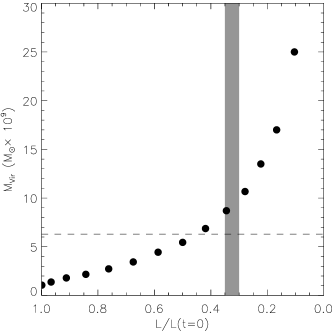
Figure 11.— Virial mass of the NFW halo at $z=0$ as a function of luminosity remaining in the core. The shaded region shows the range of luminosities determined in this paper. If we are missing light from additional wraps or apocenter pile-ups the mass quickly exceeds that of the other classical dwarfs.The dashed line indicates the virial mass of Draco (the most massive classical dwarf according to Peñarrubia et al. $2008$a).

References

- Abazajian et al. (2009) Abazajian, K. N., et al. 2009, ApJS, 182, 543
- Bellazzini et al. (2006) Bellazzini, M., Correnti, M., Ferraro, F. R., Monaco, L., & Montegriffo, P. 2006, AA, 446, L1
- Belokurov et al. (2006a) Belokurov, V., et al., 2006, ApJ, 642, L137
- Cox (1999) Cox, A. N., 1999. Allen’s Astrophysical Quantities, Springer, Berlin
- Dehnen et al. (2004) Dehnen, W., Odenkirchen, M., Grebel, E. K., & Rix, H.-W. 2004, AJ, 127, 2753
- Dotter et al. (2008) Dotter, A., Chaboyer, B., Jevremović, D., Kostov, V., Baron, E., & Ferguson, J. W. 2008, ApJS, 178, 89
- Fellhauer et al. (2006) Fellhauer, M., et al. 2006, ApJ, 651, 167
- Geha et al. (2009) Geha, M., van der Marel, R. P., Guhathakurta, P., Gilbert, K. M., Kalirai, J., & Kirby, E. N. 2009, arXiv:0911.3654
- Girardi et al. (2004) Girardi, L., Grebel, E. K., Odenkirchen, M., & Chiosi, C. 2004, AA, 422, 205
- Helmi (2004) Helmi, A. 2004, ApJ, 610, L97
- Ibata et al. (1995) Ibata, R. A., Gilmore, G., & Irwin, M. J. 1995, MNRAS, 277, 781
- Jiang & Binney (2000) Jiang, I.-G., & Binney, J. 2000, MNRAS, 314, 468
- Johnston et al. (2005) Johnston, K. V., Law, D. R., & Majewski, S. R. 2005, ApJ, 619, 800
- Jurić et al. (2008) Jurić, M., et al. 2008, ApJ, 673, 864
- Law et al. (2005) Law, D. R., Johnston, K. V., & Majewski, S. R. 2005, ApJ, 619, 807
- Law et al. (2009) Law, D. R., Majewski, S. R., & Johnston, K. V. 2009, Accepted for publication in ApJ Letters (arXiv:0908.3187)
- Majewski et al. (1999) Majewski, S. R., Siegel, M. H., Kunkel, W. E., Reid, I. N., Johnston, K. V., Thompson, I. B., Landolt, A. U., & Palma, C. 1999, AJ, 118, 1709
- Majewski et al. (2003) Majewski, S. R., Skrutskie, M. F., Weinberg, M. D., & Ostheimer, J. C. 2003, ApJ, 599, 1082
- Martínez-Delgado et al. (2001) Martínez-Delgado, D., Aparicio, A., Gómez-Flechoso, M. Á., & Carrera, R. 2001, ApJ, 549, L199
- Mateo et al. (1995) Mateo, M., Udalski, A., Szymanski, M., Kaluzny, J., Kubiak, M., Krzeminski, W. 1995, AJ, 109, 588
- Mateo (1998) Mateo, M. L. 1998, ARA&A, 36, 435
- Mateo et al. (1998) Mateo, M., Olszewski, E. W., Morrison, H. L. 1998, ApJL, 508, L55
- Newberg et al. (2002) Newberg, H. J., et al. 2002, ApJ, 569, 245
- Newberg et al. (2007) Newberg, H. J., Yanny, B., Cole, N., Beers, T. C., Re Fiorentin, P., Schneider, D. P., & Wilhelm, R. 2007, ApJ, 668, 221
- Peñarrubia et al. (2006) Peñarrubia, J., Benson, A. J., Martínez-Delgado, D., Rix, H. W., 2006, ApJ, 645, 240
- Peñarrubia et al. (2008) Peñarrubia, J., McConnachie, A. W., & Navarro, J. F., 2008a, ApJ, 672, 904
- Peñarrubia et al. (2008) Peñarrubia, J., Navarro, J. F., & McConnachie, A. W., 2008b, ApJ, 673, 226
- Schlegel, Finkbeiner, & Davis (1998) Schlegel, D.J., Finkbeiner, D.P., & Davis, M., 1998, ApJ, 500
- Sirko et al. (2004) Sirko, E., et al. 2004, AJ, 127, 899
- Skrutskie et al. (2006) Skrutskie, M. F., et al. 2006, AJ, 131, 1163
- van den Bergh (2000) van den Bergh, S., 2000. The Galaxies of the Local Group, Cambridge University Press, Cambridge
- Vivas et al. (2001) Vivas, A. K., et al. 2001, ApJ, 554, L33
- Watkins et al. (2009) Watkins, L.L. et al. 2009, MNRAS, in press (arXiv:0906.0498)
- Yanny et al. (2000) Yanny, B., et al. 2000, ApJ, 540, 825
- Yanny et al. (2009) Yanny, B., et al. 2009, ApJ, 700, 1282