Communication activity in social networks: growth and correlations

Abstract

We investigate the timing of messages sent in two online communities with respect to growth fluctuations and long-term correlations. We find that the timing of sending and receiving messages comprises pronounced long-term persistence. Considering the activity of the community members as growing entities, i.e. the cumulative number of messages sent (or received) by the individuals, we identify non-trivial scaling in the growth fluctuations which we relate to the long-term correlations. We find a connection between the scaling exponents of the growth and the long-term correlations which is supported by numerical simulations based on peaks over threshold. In addition, we find that the activity on directed links between pairs of members exhibits long-term correlations, indicating that communication activity with the most liked partners may be responsible for the long-term persistence in the timing of messages. Finally, we show that the number of messages, $M$, and the number of communication partners, $K$, of the individual members are correlated following a power-law, $K\sim M^{\lambda}$, with exponent $\lambda\approx 3/4$.

1 Introduction

Seeking for simple laws and regularities in human activity, researchers belonging to various disciplines aim to study social phenomena by describing them with methods from natural sciences. Since communication plays a predominant role in social systems, it is desired to obtain better insight into the nature of communication patterns – and therefore to understand both, communication itself and the social systems. Although it is clear that communication is related to the embedment in social networks, the actual dynamical processes are still poorly understood.

Studying economic data, surprising growth patterns have been identified StanleyABHLMSS1996 , which seem to be abundant in systems with growth-like features CanningALMS1998 ; PlerouAGMS1999 ; LiljerosF2003 ; MatiaALMS2005 ; PicoliM2008 ; RozenfeldRABSM2008 ; WangYHS2009 . Considering the units of a system of interest and calculating their logarithmic growth rates between two time steps, it was found that the standard deviation of the growth rates decays as a power-law with the initial size StanleyABHLMSS1996 . This finding represents a violation of Gibrat’s law GibratR1931 ; SuttonJ1997 ; MitzenmacherM2004 stating that the average and the standard deviation of the growth rate of a given economic indicator are constant and independent of the specific indicator value, see also RozenfeldRABSM2008 .

In a recent study RybskiBHLM2009 we have found several scaling laws characterizing the communication activity in online social networks. We found the existence of long-term correlations in human activity of sending messages to other members in the social network. The long-term persistence is related to the fluctuations in the growth properties of the social network as measured by the cumulative number of message sent by the members. The present paper expands this previous work by studying the messages sent in two online social networks with respect to the following properties. First, we extend the results obtained in RybskiBHLM2009 , revealing the analogue correlations in the timing of receiving messages. Furthermore, we analyze the temporal correlations of the activity on directed links, i.e. between pairs of members, and find almost identical results as on the level of the single members.

Second, in line with RybskiBHLM2009 we study the growth of the cumulative communication activity of the members in terms of the cumulative numbers of messages sent and received. In RybskiBHLM2009 we have shown that the standard deviation of the growth rates of the cumulative number of messages sent by individuals depend on the ’size’ of the member (defined as the cumulative numbers of messages) following a power-law with exponent $\beta\approx 0.2$, significantly different from the random exponent $\beta_{\rm rnd}=1/2$, indicating nontrivial fluctuations and persistence in the human communication activity in the social networks. Here we further study the distribution of the logarithmic growth rates and find exponential decays similarly to those encountered in econophysics StanleyABHLMSS1996 .

Third, in order to understand the relation between the long-term correlations and growth fluctuations, we propose a simulation approach based on peaks over threshold modeling. Using artificially generated long-term correlated sequences, a message is sent when the record exceeds a predefined threshold. Numerically, we measure the long-term correlations characterized by the exponent $H$ as well as growth fluctuations characterized by $\beta$ and find that the relation connecting both exponents proposed in RybskiBHLM2009 holds.

Fourth, we introduce a new growth rate between any pair of members quantifying the mutual growth in the number of messages. We find that the corresponding growth fluctuations follow a power-law with similar exponent as for the ’normal’ growth rates. We motivate that the exponent might be related to cross-correlations in the activity of the members.

Fifth, in addition to the temporal correlations, we investigate the total number of messages sent or received and the total in- and out-degree (i.e. the number of different members from which a member receives or to whom he/she sends). We find that the total degree and the final number of messages are correlated following a power-law with exponent close to $0.75$. In the case of final in- vs. out-degree, deviations from the linear correlations are found.

Finally, we point out that there is also a relation between our results on growth fluctuations and long-range correlations ($\beta$ and $H$, respectively) and the existence of power-law distributed inter-event times characterized by the exponent $\delta$ BarabasiAL2005 leading to the clustering and bursts in the activity of members. This connection is explored in a follow-up paper RybskiBHLM5a .

Our results have important implications for the design of communication systems. The correlations can be elaborated to better predict information propagation, see e.g. KarsaiKPKKBS2010 . In addition, the characterization of fluctuations is essential for the knowledge of uncertainty. Our approach could be also applied in natural systems such as in the context of protein unfolding BrujicHWF2006 .

This paper is organized as follows. In Sec. 2 we briefly describe the data of messages sent in two online communities. Our results are presented in Sec. 3 which is organized in four sub-sections – discussing long-term correlations, growth fluctuations, modeling, and other correlations. Finally, we draw our conclusions in Sec. 4.

2 Data

We analyze the timing of messages sent in two Internet communities RybskiBHLM2009 ; GallosRLHM2011 . The data of the first online community (www.qx.se, QX) consists of over $80,000$ members and more than $12.5$ million messages sent during $63$ days (mid November 2005 until mid January 2006). The data of the second online community (www.pussokram.com, POK) covers 492 days (February 2001 until June 2002) of activity with more than 500,000 messages sent among almost 30,000 members HolmeP2003 ; HolmeLEK2003 ; HolmeEL2004 . This corresponds to the entire lifespan of the social network. Both web-sites are used for dating and general social interactions. The QX community is used mainly by Swedish gay and lesbian while POK was targeted to Swedish teenagers and young adults. All data are completely anonymous, lack any message content and consist only of the time when the messages are sent and identification numbers of the senders and receivers. The advantage of these data sets is that they provide the exact time when the messages were sent – in contrast to similar network data sets consisting only of snapshots, i.e. temporally aggregated social networks expressing who sent messages to whom (see GallosRLHM2011 for a discussion).

Similarly to other online communities, the members can log in and meet virtually. There are different ways of interacting in these communities. Common among most of such online communities is the possibility to choose favorites, i.e. a list of other members, that a person somehow feels committed to. In addition, the platforms offer the possibility to join groups and discuss with other members about specific topics. We focus on the messages sent among the members. These messages are similar to e-mails but have the advantage that they are sent within a closed community where there are no messages coming from or going outside.

From the message data one can also build networks, which consist of links connecting nodes. We consider the members as nodes and set a directed link from node a to b when member a sends at least one message to b. The degree, $k$, of a node is the number of other nodes it is connected to, i.e. the number of links it has. In the directed case one distinguishes between out-degree (number of out-going links) and in-degree (number of in-going links).

3 Analysis

3.1 Long-term correlations

Figure 1: Comparison of fluctuation functions in (a) daily and (b) weekly resolution of members sending messages in POK. The different curves correspond to different activity levels: $M=$1-2, 3-7, 8-20, 21-54, 55-148, 149-403, 404-1096, 1097-2980 total messages (from bottom to top). The curves in (b) have been shifted along the $\Delta t$ axis to match daily resolution. In both cases the asymptotic scaling is the same. The dotted lines correspond to the exponents $H=1$ (top) and $H=1/2$ (bottom).

Figure 2: Fluctuation exponents of the communication activity (a) sending and (b) receiving messages by members of QX. The exponents are plotted as a function of the activity level $M$, i.e. total number of messages, for the original data (green circles), and individually shuffled sequences (orange diamonds). See also RybskiBHLM2009 .

Figure 3: Fluctuation exponents of the communication activity (a) sending and (b) receiving messages by members of POK (weekly resolution). The exponents are plotted as a function of the activity level $M$ for the original data (green circles), and individually shuffled sequences (orange diamonds). See also RybskiBHLM2009 .

First, we define the activity record, $\mu_{j}(t)$, counting the number of messages member $j$ sends at day/week $t$. Thus, we study the activity that is aggregated at the daily or weekly level. This is done to avoid possible oscillations that are observed in the data at both frequencies.

In a previous study RybskiBHLM2009 we have applied Detrended Fluctuation Analysis (DFA) PengBHSSG94 ; BundeHKPPV00 ; KantelhardtKRHB01 and found that the activity records, $\mu(t)$, exhibit long-term correlations, which are characterized by a power-law decaying auto-correlation function,

$$C(\Delta t) = \frac{1}{\sigma_{\mu}^{2}}\left\langle\left[\mu(t)-\langle\mu(t)\rangle\right]\left[\mu(t+\Delta t)-\langle\mu(t)\rangle\right]\right\rangle$$

$$\sim (\Delta t)^{-\nu}\,,$$

where $\langle\mu(t)\rangle$ is the average of the record $\mu(t)$, $\sigma_{\mu}$ is its standard deviation, and $\nu$ is the correlation exponent ($1\geq\nu\geq 0$). The fluctuation function provided by DFA scales as

$$F(\Delta t)\sim(\Delta t)^{H}$$ (1)

where the exponent $H$ is similar to the Hurst exponent ($1/2\leq H\leq 1$, larger exponents correspond to more pronounced long-term correlations). It is related to the correlation exponent via

$$\nu=2-2H\,.$$ (2)

For uncorrelated or short-term correlated records the asymptotic fluctuation exponent is $H=1/2$ (for a review we refer to KantelhardtJW2010 ).

In order to study the activity with respect to long-term correlations, we apply second order DFA (DFA2) BundeHKPPV00 ; KantelhardtKRHB01 [linear detrending of $\mu_{j}(t)$] and obtain the fluctuation functions, $F^{j}_{\rm DFA2}(\Delta t)$ (details can be found in RybskiBHLM2009 ). Since the activity records of the individual members are too short, we average the squared fluctuation functions among members with similar overall activity (i.e. total number of messages, $M$): $F(\Delta t)=[\sum_{j|M}(F^{j}(\Delta t))^{2}]^{1/2}$. Therefore, we employ logarithmic bins in $M$. The activity distributions are discussed in Sec. 3.4.1.

In Fig. 1 we compare for sending in POK the fluctuation functions in daily resolution [Fig. 1(a)] and weekly resolution [Fig. 1(b)]. In order to match the scales, we have shifted the curves in Fig. 1(b) along the $\Delta t$-axis. Naturally, in daily resolution, the fluctuation functions cover more scales. The asymptotic scaling is in both cases the same, namely no correlations in the case of least active members and strong long-term correlations with fluctuation exponents close to $1$ for the most active members. Moreover, for POK in daily resolution, the fluctuation functions exhibit an increase from small slopes on short time scales to larger slopes on large scales. This indicates that the long-term correlations do not vanish after certain scale, but the opposite, the long-term correlations become stronger. Note, that we use weekly resolution in order to cope with possible weekly oscillations GolderWH2006 ; LeskovecH2008 ; MalmgrenSMA2008 .

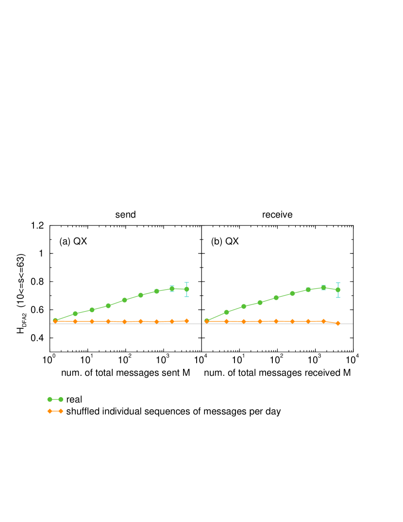
We measure the fluctuation exponents by applying least squares fits to $\log F(\Delta t)$ vs. $\log\Delta t$ on the scales $10<\Delta t<63$ days (QX) and $10<\Delta t<70$ weeks (POK). For the former case the obtained fluctuation exponents are plotted in Fig. 2 as a function of the members activity level, i.e. their total number of messages $M$. For sending [panel (a)], the less active members exhibit uncorrelated behavior. The more messages the members send overall, the stronger correlated is their activity. The fluctuation exponent $H_{\rm QX}$ increases with $M$ and reaches values up to $0.75\pm 0.05$ (sending). In contrast, for the shuffled data, the fluctuation exponents are always very close to $1/2$. This confirms that the long-term correlations are due to the temporal structure of the times each member sends his/her messages, see also RybskiBHLM5a . For receiving messages, Fig. 2(b), we find almost identical results. The error bars in Fig. 2 were calculated by subdividing the groups of different activity level. The size of the error bars is simply the standard deviation of the corresponding exponents.

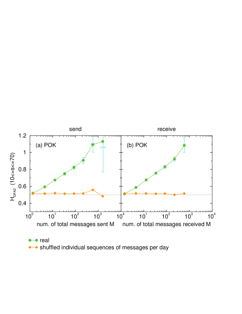
The estimated fluctuation exponents obtained for POK are displayed in Fig. 3. Qualitatively, we obtain a similar picture as for QX. However, in contrast to QX, here the original records achieve larger fluctuation exponents up to $0.91\pm 0.04$ (sending), disregarding the last points which carry large error-bars. A possible reason for these different maximum exponents could be that in the case of POK the data covers a much longer period of data acquisition, and possible non-stationarities VazquezA2007 . In QX, the members might not have had enough time to exhibit the full extend of their persistence, while in POK we follow the entire evolution of the online community.

Indeed, similar behavior of long-term correlations have been found in traded values of stocks and e-mail communication EislerK2006 ; EislerBK2008 , where the fluctuation exponent increases in an analogous way with the mean trading activity of the corresponding stock or with the average number of e-mails (see also RochaLH2010 ).

Apart from these, for human related data, long-term persistence has been reported for physiological records PengMHHSG1993 ; IvanovBAHFBSG1999 ; BundeHKPPV00 , written language KosmidisKA2006 , or for records generated by collective behavior such as finance and economy LiuGCMPS1999 ; MantegnaS1999 ; LuxA2002 , Ethernet traffic LelandTWW1994 , Wikipedia access KaempfTKM2011 , as well as highway traffic TadakiKNNSSY2006 ; XiaoYanZHM2007 . There are also indications of long-term correlations in human brain activity LinkenkaerHansenNPI2001 ; AllegriniMBFGGWP2009 and human motor activity IvanovHHSS2007 .

A question that arises is, why the fluctuation exponent (in Figs. 2 and 3) depends on the activity level of the members, that is, why the least active members exhibit no persistence while the most active members exhibit strong persistence. We argue that if only few messages appear in the whole period of data acquisition, long-term persistence cannot be reflected. In these cases it is quite possible that much longer records and higher aggregation level such as months or years would be needed to reveal the persistence. But doing so, there would be other members with even less messages which then again would probably appear with seemingly uncorrelated message signals. Thus, we propose that the exponents of the largest activity reflect more accurately the scaling behavior of human communication activity. In Sec. 3.3.1 we propose statistical simulations to generate data using peaks over threshold (POT) and find that it supports this perception.

Figure 4: Temporal correlations in the daily amount of messages on directed links in QX. (a) DFA2 fluctuation functions versus the time scale $\Delta t$, averaged conditional to the final number of messages of each link. The different curves correspond to different activity levels: $M_{\rm L}=$1-2, 3-7, 8-20, 21-54, 55-148, 149-403, 404-1096, 1097-2980 (from bottom to top). The dotted lines correspond to the exponents $H=0.75$ (top) and $H=1/2$ (bottom). (b) The DFA2 fluctuation exponent $H_{\rm L,QX}$ obtained from (a) is plotted as a function of the activity level $M_{\rm L}$. The exponents were obtained in the range of scales $10\leq\Delta t\leq 63$ days. The activity along directed links comprise similar long-term correlations as the total activity of individual members to all of their acquaintances.

At this point we need to mention that long-term correlations can be related to broad inter-event time distributions, i.e. the times between successive messages of individual members. Such distributions have been investigated, see e.g. BarabasiAL2005 ; MalmgrenSCA2009 , but there is no consensus on the functional form. We study the inter-event time distributions in a different publication RybskiBHLM5a where we demonstrate the connection with the long-term correlations found here.

Along directed links

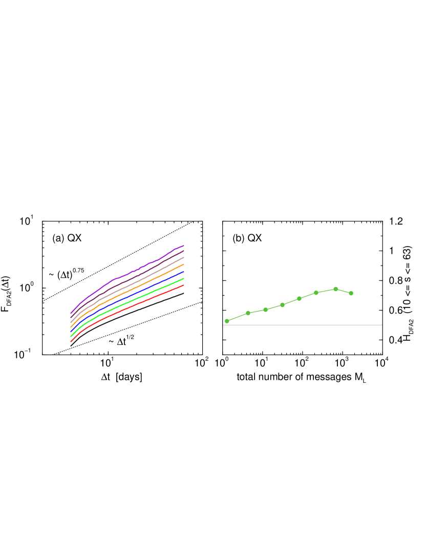
In Fig. 4 we study for QX the long-term correlations in activity not on the sender or receiver (node) level but on the level of messages along directed links. This means that we track when a message is sent directed between two members but separately for any pair of members, such as a$\rightarrow$b, b$\rightarrow$a, a$\rightarrow$d, …. Accordingly, we determine the activity records $\mu_{\texttt{ab}}(t)$, $\mu_{\texttt{ba}}(t)$, $\mu_{\texttt{ad}}(t)$, etc., expressing how many messages have been sent each day/week, $t$, between any pair of members. Analogous, there is also an activity level for the links, $M^{\texttt{ab}}_{\rm L}$, …(we disregard those pairings without activity). Then we perform the analogous analysis for long-term correlations by applying DFA2 and averaging among pairings with similar overall activity (the distributions of activity are discussed in Sec. 3.4.1). The fluctuation functions in Fig. 4(a) have asymptotic slopes close to $1/2$ for those links with few total number of messages. In contrary, those links with many total number of messages exhibit long-term correlations with exponents up to $0.74$. The fluctuation exponents as a function of the activity level $M_{\rm L}$ are plotted in Fig. 4(b). Apart from the fact, that by definition the number of messages on the most active links is lower (or equal) than the number of messages of the most active members, the curve looks very similar to the one in Fig. 2(a), in particular the maximum exponents are quite similar ($H_{\rm QX}\approx 0.75$ and $H_{\rm L,QX}\approx 0.74$). This indicates, that the persistence in the communication may be dominated by the communication activity with the most liked partners.

In HidalgoR2008 a different concept of persistence links has been investigated. The period of data acquisition is partitioned into time slices in each of which a network is built. Then the persistence is defined as the normalized number of time slices in which a certain link appears. However, the approach of our work is not compatible with the one in HidalgoR2008 and we cannot directly compare the results.

3.2 Growth process

3.2.1 Growth in the number of messages

As suggested in RybskiBHLM2009 we also analyze the growth properties of the message activity. This concept is borrowed from econophysics, where the growth of companies has been found to exhibit non-trivial scaling laws StanleyABHLMSS1996 , that in particular violate the original Gibrat’s law GibratR1931 ; SuttonJ1997 ; MitzenmacherM2004 ; SaichevMS2009 and at the same time represents a generalized Gibrat’s law (GGL) RybskiBHLM2009 . In the present study, each member is considered as a unit and the number of messages sent or received since the beginning of data acquisition represents its size. We analyze the growth in the number of messages in analogy to other systems such as the growth of companies StanleyABHLMSS1996 ; AmaralBHSS1998 or the growth of cities RozenfeldRABSM2008 ; RozenfeldRGM2009 . The analogy is supported by some aspects: (i) The members of a community represent a population similar to the population of a country. (ii) The number of members fluctuates and typically grows analogous to the number of cities of a country. (iii) The activity or number of links of individuals fluctuates and grows similar to the size of cities.

The cumulative number, $m^{j}(t)$, expresses how many messages have been sent by a certain member $j$ up to a given time $t$ [for a better readability we will not write the index $j$ explicitly, $m(t)$]. We consider the evolution of $m(t)$ between times $t_{0}$ and $t_{1}$ within the period of data acquisition $T$ ($t_{0}<t_{1}\leq T$) as a growth process, where each member exhibits a specific growth rate $r_{j}$ ($r$ for short notation):

$$r=\ln\frac{m_{1}}{m_{0}}\,,$$ (3)

where $m_{0}\equiv m(t_{0})$ and $m_{1}\equiv m(t_{1})$ are the number of messages sent until $t_{0}$ and $t_{1}$, respectively, by every member. To characterize the dynamics of the activity, we consider two measures. (i) The conditional average growth rate, $\langle r(m_{0})\rangle$, quantifies the average growth of the number of messages sent by the members between $t_{0}$ and $t_{1}$ depending on the initial number of messages, $m_{0}$. In other words, we consider the average growth rate of only those members that have sent $m_{0}$ messages until $t_{0}$. (ii) The conditional standard deviation of the growth rate for those members that have sent $m_{0}$ messages until $t_{0}$,

$$\sigma(m_{0})\equiv\sqrt{\langle(r(m_{0})-\langle r(m_{0})\rangle)^{2}\rangle}\,,$$ (4)

expresses the statistical spread or fluctuation of growth among the members depending on $m_{0}$. Both quantities are relevant in the context of Gibrat’s law in economics GibratR1931 ; SuttonJ1997 ; MitzenmacherM2004 ; SaichevMS2009 which proposes a proportionate growth process entailing the assumption that the average and the standard deviation of the growth rate of a given economic indicator are constant and independent of the specific indicator value. That is, both $\langle r(m_{0})\rangle$ and $\sigma(m_{0})$ are independent of $m_{0}$.

As shown in RybskiBHLM2009 , for the message data the conditional average growth rate is almost constant and only decreases slightly,

$$\langle r(m_{0})\rangle\sim m_{0}^{-\alpha}\,,$$ (5)

with an exponent $\alpha\approx 0.05$. This means that members with many messages in average increase their number of messages almost with the same rate as members with few messages. In contrast, the conditional standard deviation clearly decreases with increasing $m_{0}$,

$$\sigma(m_{0})\sim m_{0}^{-\beta}\,,$$ (6)

where $t_{0}=T/2$ is optimal in terms statistics. In this case the exponents $\beta_{\rm QX}=0.22\pm 0.01$ and $\beta_{\rm POK}=0.17\pm 0.03$ for sending messages were found RybskiBHLM2009 . This means, although the average growth rate almost does not depend on $m_{0}$, the conditional standard deviation of the growth of members with many messages is smaller than the one of members with few messages. Due to weaker fluctuations, active members are relatively better predictable in their activity of sending messages.

It has been shown that the fluctuation exponent $H$ and the growth fluctuation exponent $\beta$ are related via RybskiBHLM2009

$$\beta=1-H\,.$$ (7)

Equation (7) is a scaling law formalizing the relation between growth and long-term correlations in the activity. According to Eq. (7), the original Gibrat’s law ($\beta_{\rm G}=0$) corresponds to very strong long-term correlations with $H_{\rm G}=1$. In contrast, $\beta_{\rm rnd}=1/2$ represents completely random activity $(H_{\rm rnd}=1/2)$. The observed message data comprises $1/2>\beta>0$ and $1/2<H<1$. Surprisingly, the values of $\beta$ found here are very close to the $\beta$ values found for companies in the US economy StanleyABHLMSS1996 .

In the case of companies, also the distribution of growth rates has been studied. It was found that the distribution density follows StanleyABHLMSS1996 :

$$p(r|m_{0})=\frac{1}{s\sigma(m_{0})}\exp\!\left(-\frac{s|r-\langle r(m_{0})\rangle|}{\sigma(m_{0})}\right)\,,$$ (8)

whereas $s=\sqrt{2}$. Next we analyze, how the growth rates $r$ are distributed in the case of the message data.

First we need to point out that in contrast to the growth of companies, our entities can never shrink. The members cannot loose messages, the number $m(t)$ either increases or remains the same. Accordingly, in our case $r\geq 0$ and therefore $s=1$, as can be derived for the single-sided exponentially decaying distribution.

Figure 5: Scaled probability density of growth rates $r$, Eq. (3), in the number of messages by members of QX. (a) Sending and (b) receiving. The times for $m_{0}$ and $m_{1}$ have been chosen as $t_{0}=T/2$ and $t_{1}=T$. The symbols correspond to different initial number of messages $m_{0}$. The axis are scaled assuming a distribution according to Eq. (8) with $s=1$ which then corresponds to the dotted lines.

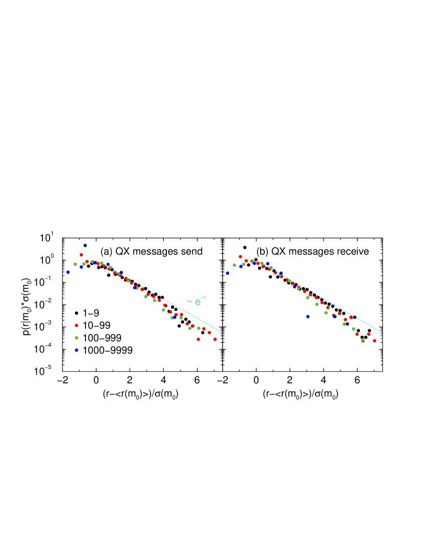
Figure 5 shows $p(r|m_{0})$ for QX where the values are scaled to collapse according to Eq. (8) with $s=1$. In order to have reasonable statistics, we define the condition $m_{0}$ in rather wide ranges, namely according to the decimal logarithm. For sending [Fig. 5(a)] and receiving [Fig. 5(b)] messages the scaled probability densities collapse and are quite similar. Nevertheless, the growth rates do not exactly follow Eq. (8) with $s=1$. While for the less active members with small growth rates we find a good agreement, for more active members and large growth rates the obtained curves deviate from the theoretical one towards a steeper decay.

Figure 6: Scaled probability density of growth rates $r$, Eq. (3), in the number of messages by members of POK. (a) Sending and (b) receiving. Analogous to Fig. 5.

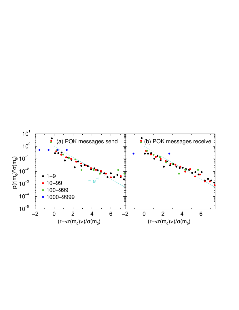
The corresponding results for POK are shown in Fig. 6. Again, sending and receiving are very similar. The curves collapse reasonably, but in contrast to QX here the measured $p(r|m_{0})$ overall deviate from the theoretical one comprising less steep slopes.

We argue that as for single time series, distribution and correlation properties are in most cases independent, the same holds for the message data and the growth. The distribution of growth rates $p(r|m_{0})$ seems to be independent from the long-term correlations which are reflected in $\sigma(m_{0})$ with the exponent $\beta$.

3.2.2 Mutual growth in the number of messages

Next we study a variation of growth. Instead of considering the absolute number of messages a member sends, we study the difference in the number of messages compared to any other member, the mutual difference $m^{i}(t)-m^{j}(t)$. Thus, the growth rate is defined analogous to Eq. (3)

$$r_{\times}=\ln\frac{m_{1}^{i}-m_{1}^{j}}{m_{0}^{i}-m_{0}^{j}}$$ (9)

where now there is a growth rate for every pair of members $i$ and $j$. The conditional average growth rate and the corresponding standard deviation is then taken over all possible pairs and the condition is the difference at $t_{0}$, $m^{i}_{0}-m^{j}_{0}=m^{i}(t_{0})-m^{j}(t_{0})$, providing the quantities $\langle r_{\times}(m^{i}_{0}-m^{j}_{0})\rangle$ and $\sigma(m^{i}_{0}-m^{j}_{0})$. We disregard combinations of $i$ and $j$ where $m_{0}^{i}-m_{0}^{j}=0$ or $\frac{m_{1}^{i}-m_{1}^{j}}{m_{0}^{i}-m_{0}^{j}}\leq 0$.

Figure 7: Average mutual growth rate and standard deviation versus foregoing difference in the number of messages for sending in QX. The average (open squares) and standard deviation (filled circles) of the mutual growth rate $r_{\times}$, Eq. (9), are plotted conditional to the initial difference $m_{0}^{i}-m_{0}^{j}$, whereas $t_{0}=T/2$ and $t_{1}=T$. (a) Original data and (b) shuffled data. The dotted line in (a) corresponds to the exponent $\beta_{\times}=0.3$ and in (b) to $\beta_{\times}=1/2$.

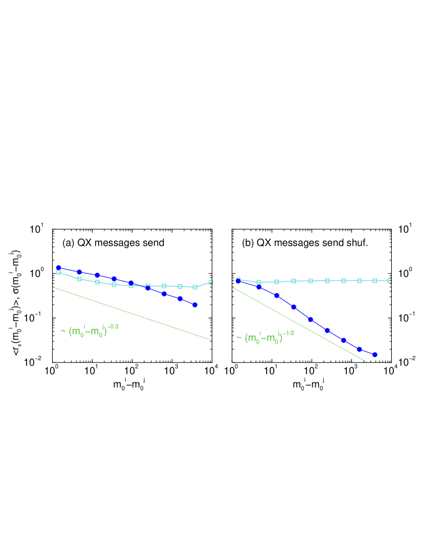
The results for sending in QX are shown in Fig. 7. Apart from a small decrease up to $m^{i}_{0}-m^{j}_{0}\approx 50$, the average growth rate is constant [Fig. 7(a)]. The conditional standard deviation asymptotically follows a slope $\beta_{\times}\approx 0.3$ with deviations to small exponents for small $m^{i}_{0}-m^{j}_{0}$. In the case of the shuffled data [Fig. 7(b)], as expected, the average growth rate is constant while the standard deviation decreases steeper than for the original data, namely with $\beta_{\times,{\rm rnd}}\simeq 1/2$, although not with a nice straight line. Nevertheless, we conclude that the scaling of the standard deviation in Fig. 7(a) must be due to temporal correlations between the members. The growth of the difference between their number of messages comprises similar scaling as the individual growth.

We conjecture that $\sigma(m^{i}_{0}-m^{j}_{0})$ reflects long-term cross-correlations in analogy to $\sigma(m_{0})$ for auto-correlations. However, so far, we are not able to provide further evidence for this analogy and the corresponding relation to $\beta=1-H$, Eq. (7), since an appropriate technique for the direct quantification of long-term cross-correlations is lacking.

3.3 Modeling

In what follows, we propose numerical simulations with the purpose of testing the methods and empirical patterns we found. We study three approaches adopted to the modeling of human activity: (a) peaks over thresholds, (b) preferential attachment BarabasiA1999 , and (c) cascading Poisson process MalmgrenSMA2008 .

3.3.1 Peaks over threshold (POT) simulations

Our finding that the activity of sending messages exhibits long-term persistence asserts the existence of an underlying long-term correlated process. This can be understood as an unknown individual state driven by various internal and external stimuli HedstroemP2005 ; KentsisA2006 ; PallaBV2007 ; CraneS2008 ; MalmgrenSMA2008 ; AllegriniMBFGGWP2009 increasing the probability to send messages. Generating such a hypothetical long-term correlated internal process $(x_{i})$, simulated message data can be defined by the instants at which this internal process exceeds a threshold $q$ (peaks over threshold, POT), see BundeEKH2005 ; AltmannK2005 ; EichnerKBH2007 and references therein.

More precisely, we consider a long-term correlated sequence $(x_{i})$ consisting of $N^{*}$ random numbers that is normalized to zero average ($\langle x\rangle=0$) and unit standard deviation ($\sigma_{x}=1$). Choosing a threshold $q$, at each instant $i$ the probability to send a messages is:

$$p_{\rm snd}=\left\{\begin{array}[]{cl}1&\mbox{ for }x_{i}>q\\ 0&\mbox{ for }x_{i}\leq q\end{array}\right.\,.$$ (10)

Thus, the message events are given by the indices $i$ of those random numbers $x_{i}$ exceeding $q$.

Figure 8: Illustration of the peaks over threshold simulations. (a) An underlying and unknown long-term correlated process determines the instantaneous probability of sending messages. Once this state passes certain threshold $q$ (dashed orange line) a messages is sent (green diamonds). (b) Generated instants of messages, (c) with windows for aggregation, such as messages per day. (d) Aggregated record of messages in windows of size $w$, here $w=10$.

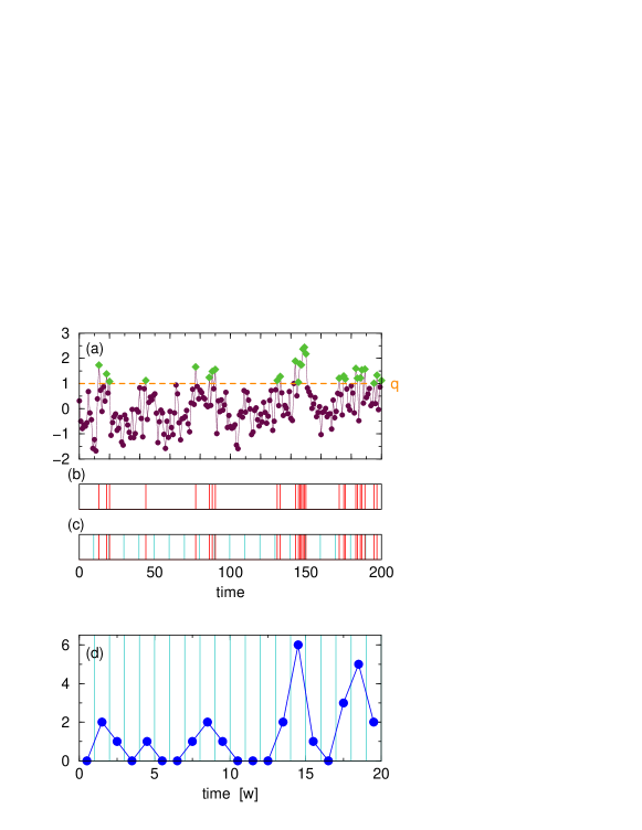
Figure 8(a) illustrates the procedure. The random numbers are plotted as brown circles and the events exceeding the threshold (orange dashed line) by the green diamonds. The resulting instants are depicted in Fig. 8(b) representing the simulated messages. The threshold approximately predefines the total number of events and accordingly the average inter-event time. Using normal-distributed numbers $(x_{i})$, the number of events/messages is approximately given by the length $N^{*}$ and the inverse cumulative distribution function associated with the standard normal distribution (probit-function). Additionally, the random numbers we use are long-term correlated with variable fluctuation exponent. We impose these auto-correlations using Fourier Filtering Method KantelhardtKRHB01 ; MakseHSS96 . Next we show that this process reproduces the scaling in the growth, i.e. GGL, as well as the variable long-term correlations in the activity of the members (e.g. Figs. 2 and 3).

Figure 9: Results of numerical simulations. (a) Mean growth rate conditional to the number of events until $t_{0}=N^{*}/2$ as obtained from $100,000$ long-term correlated records of length $N^{*}=131,072$ with variable imposed fluctuation exponent $H_{\rm imp}$ between $1/2$ and $0.9$ and random threshold $q$ between $1.0$ and $6.0$. (b) As before but standard deviation conditional to the number of events. The solid lines represent power-laws with exponents $\beta$ expected from the imposed long-term correlations according to Eq. (7). (c) Long-term correlations in the sequences of aggregated peaks over threshold. For every threshold $q$ between $1.0$ (violet) and $4.5$ (black) $100$ normalized records of length $N^{*}=4,194,304$ have been created with $H_{\rm imp}=0.9$. The events are aggregated in windows of size $w=100$. The panel shows the averaged DFA2 fluctuation functions. (d) Fluctuation exponents on the scales $1,000\leq s\leq 10,000$, as a function of the total number of events.

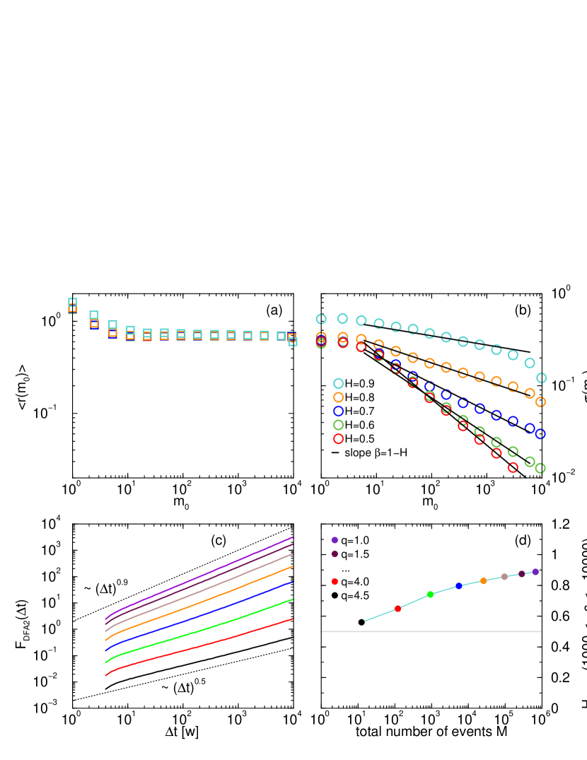
For testing this process we create 100,000 independent long-term correlated records $(x_{i})$ of length $N^{*}=131,072$, impose the fluctuation exponent $H_{\rm imp}$, and choose for each one a random threshold $q$ between $1$ and $6$, each representing a sender. Extracting the peaks over threshold, we obtain the events and determine for each record/member the growth in the number of events/messages between $N^{*}/2$ and $N^{*}$. This is, for each record/member we count the numbers of events/messages $m_{0}$ until $t_{0}=t_{i=N^{*}/2}$ as well as $m_{1}$ until $t_{1}=t_{i=N^{*}}$ and calculate the growth rate according to Eq. (3). We then calculate the conditional average $\langle r(m_{0})\rangle$ and the conditional standard deviation $\sigma(m_{0})$ where the values of $m_{0}$ are binned logarithmically. The quantities are plotted in Fig. 9(a) and (b), while in panel (b) we include slopes expected from $\beta=1-H$, Eq. (7). We find that the numerical results reasonably agree with the prediction (solid lines). Except for small $m_{0}$, these results are consistent with those found in the original message data.

The fluctuation functions can be studied in the same way. As described in Sec. 3.1, we find long-term correlations in the sequences of messages per day or per week. On the basis of the above explained simulated messages, we analyze them in an analogous way. For each threshold $q=1.0,1.5,\dots 4.0,4.5$ we create $100$ long-term correlated records of length $N^{*}=4,194,304$ with imposed fluctuation exponent $H_{\rm imp}=0.9$, extract the simulated message events, and aggregate them in non-overlapping windows of size $w=100$. This is, tiling $N^{*}$ in segments of size $w$ and counting the number of events occurring in each segment [Fig. 8(c) and (d)]. The obtained aggregated records represent the analogous of messages per day or per week and are analyzed with DFA averaging the fluctuation functions among those configurations with the same threshold and thus similar number of total events. The corresponding results are shown in Fig. 9(c) and (d). We obtain very similar results as in the original data. We find vanishing correlations for the sequences with few events (large $q$) and pronounced long-term correlations for the cases of many events (small $q$), while the maximum fluctuation exponent corresponds to the chosen $H_{\rm imp}$. This can be understood by the fact that for $q$ close to zero the sequence of number of events per window converges to the aggregated sequence of $0$ or $1$ (for $x\leq 0$ or $x>0$) reflecting the same long-term correlation properties as the original record XuYMSBI2010 . For a large threshold $q$ too few events occur to measure the correct long-term correlations, e.g. the true scaling only turns out on larger unaccessible time scales requiring larger $w$ and longer records.

Although the simulations do not reveal the origin of the long-term correlated patchy behavior, they support Eq. (7) and the concept of an underlying long-term correlated process. Consistently, an uncorrelated, completely random, underlying process recovers Poisson statistics and therefore $\beta_{\rm rnd}=1/2$ for the growth fluctuations as well as uncorrelated message activity ($H_{\rm rnd}=1/2$). For $1/2<H<1$ it has been shown BundeEKH2005 ; EichnerKBH2007 that the inter-event times follow a stretched exponential, see also BarabasiAL2005 ; StehleBB2010 ; RybskiBHLM5a .

3.3.2 Preferential attachment

Next we compare our findings with the growth properties of a network model. We investigate the Barabasi-Albert (BA) model which is based on preferential attachment and has been introduced to generate a kind of scale-free networks BarabasiA1999 ; AlbertB2002 with power-law degree distribution $p(k)$ EbelMB2002 ; NewmanFB2002 , whereas the degree $k$ of a node is the number of links it has to other ones. Essentially, it consists of subsequently adding nodes to the network by linking them to existing nodes which are chosen randomly with a probability proportional to their degree.

We obtain the undirected network and study the degree growth properties by calculating the conditional average growth rate $\langle r_{\rm BA}(k_{0})\rangle$ and the conditional standard deviation $\sigma_{\rm BA}(k_{0})$ obtained from the scale-free BA model. The times $t_{0}$ and $t_{1}$ are defined by the number of nodes attached to the network.

Figure 10: Average degree growth rate and standard deviation versus foregoing degree for the preferential attachment network model BarabasiA1999 . The average (green open diamonds) and standard deviation (blue filled circles) of the growth rate $r_{\rm BA}$ are plotted conditional to $k_{0}$, the degree of the corresponding nodes at the first stage. We choose average degree $\langle k\rangle=20$, $50,000$ nodes in $t_{0}$, and $100,000$ nodes in $t_{1}$. The error-bars are taken from $10$ configurations. The dashed line in the bottom corresponds to $\beta_{\rm BA}=1/2$.

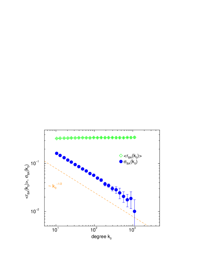
Figure 10 shows the results where an average degree $\langle k\rangle=20$; $50,000$ nodes in $t_{0}$, and $100,000$ nodes in $t_{1}$ were chosen. We find constant average growth rate that does not depend on the initial degree $k_{0}$. The conditional standard deviation is a function of $k_{0}$ and exhibits a power-law decay with $\beta_{\rm BA}=1/2$ as expected for such an uncorrelated growth process RybskiBHLM2009 . Therefore, a purely preferential attachment type of growth is not sufficient to describe the type of social network dynamics found in Sec. 3.2.1, since additional temporal correlations are involved in the dynamics of establishing acquaintances in the community.

The value $\beta_{\rm BA}=1/2$ in Eq. (7) corresponds to $H=1/2$ indicating complete randomness. There is no memory in the system. Since each addition of a new node is completely independent from precedent ones, there cannot be temporal correlations in the activity of adding links. In contrast, for the out-degree in QX and POK we obtained $\beta_{k,{\rm QX}}=0.22\pm 0.02$ and $\beta_{k,{\rm POK}}=0.17\pm 0.08$ RybskiBHLM2009 , which is supported by the (non-linear) correlations between the number of messages and the out-degree as presented in Sec. 3.4.

Interestingly, an extension of the standard BA model has been proposed BianconiB2001 , see also BlasioSL2007 ; CohenH2009 , that takes into account different fitnesses of the nodes to acquiring links. We think that such fitness could be related to growth fluctuations, thus providing a route to modify the BA model to include the long-term correlated dynamics found here.

3.3.3 Cascading Poisson process

In this Section we elaborate the model proposed in MalmgrenSMA2008 and examine it with respect to long-term correlations. The model is based on a cascading Poisson process (CPP), according to which the probability that a member enters an active interval is $\rho(t)=N_{\rm w}p_{\rm d}(t)p_{\rm w}(t)$, where $N_{\rm w}$ is the average number of active intervals per week, $p_{\rm d}(t)$ is the probability of starting an active interval at a particular time of the day, and $p_{\rm w}(t)$ is the probability of starting an active interval at a particular day of the week. Once a member enters such an active interval he/she sends a set of $N_{\rm a}+1$ messages, where $N_{\rm a}$ is drawn from the distribution $p(N_{\rm a})$. The messages sent in such an active interval are sent randomly, i.e. a homogeneous Poisson process with rate $\rho_{\rm a}$ events per hour.

Figure 11: DFA fluctuation functions of message data created with the model proposed in MalmgrenSMA2008 . (a) User 2881. We visually extract the model parameters from Fig. 3 in MalmgrenSMA2008 and generate message data for approx. $800$k days. The panel shows the fluctuation functions from DFA1 and DFA2, which asymptotically go as $\sim(\Delta t)^{1/2}$, i.e. no long-term correlations. The hump on small scales is due to the model inherent oscillations KantelhardtKRHB01 . The dashed vertical line is placed at $\Delta t=83$ days. (b) Random parameterization. We randomly choose the model parameters, create $20$k records of $83$ days and average the obtained DFA2 fluctuation functions according to the final number of messages, $M$. While for those simulated members with few messages we find $F(\Delta t)\sim(\Delta t)^{1/2}$, the $F(\Delta t)$ of the most active members exhibit a hump due to oscillations similar to the one in panel (a).

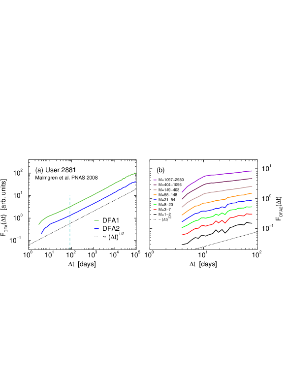
First, we study the example of User 2881 as analyzed in MalmgrenSMA2008 (please note that in MalmgrenSMA2008 a different data set is studied and the user is neither in OC1 nor in OC2). We extract from MalmgrenSMA2008 the parameters $N_{\rm w}=7.3$ active intervals per week, $\rho_{\rm a}=1.7$ events per hour, as well as (visually) the distributions $p_{\rm d}(t)$, $p_{\rm w}(t)$, and $p(N_{\rm a})$. The original period of 83 days is not sufficient to apply DFA and we run the model for this set of parameters over $800$k days. Then we extract the record of number of messages per day, $\mu(t)$, and apply DFA. The obtained fluctuation functions are shown in Fig. 11(a). On small scales below $100$ days a hump in the $F(\Delta t)$ can be identified, which is due to oscillations in $\mu(t)$ KantelhardtKRHB01 . While asymptotically the influence of oscillations vanishes, on scales below the wavelength, the oscillations appear as correlations [increased slope in $F(\Delta t)$] and on scales above the wavelength, the oscillations appear as anti-correlations [decreased slope in $F(\Delta t)$]. Asymptotically, we find $F(\Delta t)\sim(\Delta t)^{1/2}$, i.e. $H_{\rm CPP}\simeq 1/2$, corresponding to a lack of long-term correlations. Even on scales up to $83$ days, we rather find $H_{\rm CPP}<1/2$ (which we expect from the imposed weekly oscillations).

Next, we study 20,000 simulated e-mail senders with randomly chosen parameters. (i) We fill $p_{\rm w}(t)$ with random numbers and set $p_{\rm w}(t)=0$ for $t=0,6$, i.e. Sunday and Saturday. (ii) We fill $p_{\rm d}(t)$ with random numbers and set $p_{\rm d}(t)=0$ for $t=0\dots 5$ and $t=23$, i.e. at night. (iii) We set $p(N_{\rm a})$ starting with a random $p(N_{\rm a}=0)$. Then $p(N_{\rm a})$ decays exponentially up to a random $N_{\rm a}$ below $36$. $p_{\rm w}(t)$, $p_{\rm w}(t)=0$, and $p(N_{\rm a})$ are normalized. (iv) We randomly choose $0<N_{\rm w}<40$. (v) We randomly choose $0<\rho_{\rm a}<30$. From MalmgrenSMA2008 Supporting Information 2 (SI2) we estimated the typical maximum values of $N_{\rm a}$, $N_{\rm w}$, and $\rho_{\rm a}$ ($36$, $40$, and $30$, respectively). We run the model for $83$ days and extract the $\mu(t)$ for each simulated e-mail sender. Then we apply DFA2 and average the fluctuation functions according to the final number of messages, $M$, see also RybskiBHLM2009 . The fluctuation functions for the various activity levels are depicted in Fig. 11(b). We find that members with small final number of messages exhibit uncorrelated behavior. The more active the members the more pronounced become the oscillations which we already discussed in the context of Fig. 11(a). Thus, asymptotic $H_{\rm CPP}<1/2$ for large $M$ is due to the weekly cycles KantelhardtKRHB01 . In our data, oscillations do not dominate the DFA fluctuation functions. Moreover, for OC2 we also find long-term correlations in weekly resolution (Fig. 1).

Based on periodic probabilities and Poisson statistics, the CPP model represents a powerful concept to characterize inter-event times. For this purpose, the average $N_{\rm w}$ seems to be sufficient. However, in order to recover long-term correlations, time dependent $N_{\rm w}=N_{\rm w}(t)$ seem to be necessary. In fact, the number of active intervals per week, $N_{\rm w}$, fluctuates, as can be seen in MalmgrenSMA2008 SI2 (upper most row of the panels). Thus, we suggest to extend the model by introducing a memory kernel, see e.g. CraneS2008 , or by using long-term correlated $N_{\rm w}(t)$.

3.4 Other correlations

Figure 12: Correlations between the final degree $K$ and the final number of messages $M$ for QX. (a) Out-degree and sending messages; (b) in-degree and receiving messages. The dashed lines correspond to a power-law with exponent $0.75$. Members sending many messages also tend to have high out-degree, but not linearly, rather following a power-law.

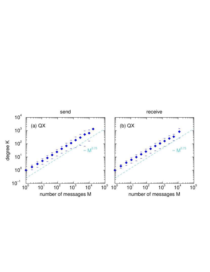
In this Section we want to discuss other types of correlations. Figure 12 shows for QX the final degree $K=k(T)$ versus the final number of messages $M=m(T)$. We find that for both, sending and receiving, the two quantities are correlated according to:

$$K\sim M^{\lambda}\quad\rm{with}\quad\lambda\approx 3/4$$ (11)

Similar relations have also been found for other data MuchnikMH2010 . Since the correlations are positive, those members that send many messages, in average, also have more acquaintances to whom they send, but they know less acquaintances than they would in the case of linear correlations. For receiving, Fig. 12(b), this correlation is very similar.

Figure 13: Correlations between activity and passivity for QX. (a) Final number of messages $M$ received and sent; (b) final in- and out-degree. The dashed lines correspond to a linear relation. Those members who send many messages also receive many. But, those members who know many people to whom they send messages do not necessarily know as many people from whom they receive messages.

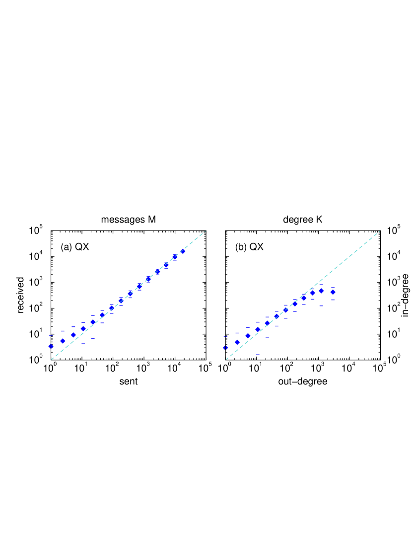
The number of messages sent versus the number of messages received (for QX) is displayed in Fig. 13(a). Asymptotically the activity and passivity are linearly related and on average for every message sent there is a received one or vice versa. This, of course, does not mean that every message is replied. However, the less active members in average tend to receive more messages than they send. For example, those members who send in average one message receive about three. Nevertheless, the more active the members are the more the sending and receiving behavior approaches the linear relation. In contrast, for the degree, Fig. 13(b), the asymptotic linear relation does not hold. Those members with large out-degree and small in-degree are referred to as spammers, since they send to many different people but only receive from few.

Figure 14: Correlations between the final degree $K$ and the final number of messages $M$ for POK. (a) Out-degree and sending messages; (b) in-degree and receiving messages. Analogous to Fig. 12.

Figure 15: Correlations between activity and passivity for POK. (a) Final number of messages $M$ received and sent; (b) final in- and out-degree. Analogous to Fig. 13

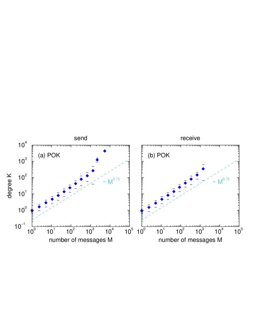
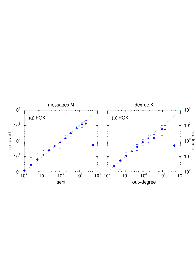
For POK we find similar results in Figs. 14 and 15. The final degree and the final number of messages also scale with an exponent close to $0.75$, although for sending messages there exist some deviations of the most active members [Fig. 14(a)]. Also, the correlations of sending and receiving are linear, the same holds for in- and out-degree. However, the most active members again deviate with low receiving part, i.e. both low number of received messages as well as low in-degree, Fig. 15. Nevertheless, the results for both data sets are mainly consistent and the power-law relation Eq. (11) is a remarkable regularity.

3.4.1 Activity and degree distributions

Figure 16: Probability densities of activities and degrees. The probabilities are plotted versus the total number of messages, $M$, and the final degree, $K$, for (a) sending in QX and (b) sending in POK. The panel (c) and (d) exhibit the probability densities of the total number of messages along directed links, $M_{L}$, for QX and POK, respectively. The dotted lines serve as guides to the eye and have the indicated slopes.

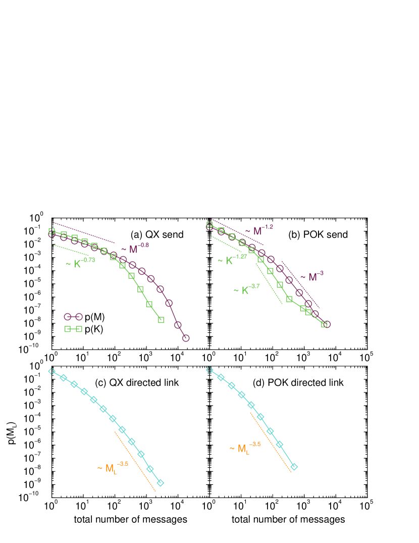
Finally, we want to briefly discuss the distributions of activities and degrees. If we assume $p(M)\sim M^{-\gamma_{M}}$ and $p(K)\sim K^{-\gamma_{K}}$, then with Eq. (11) the exponents should be related according to

$$\gamma_{K}=1+(\gamma_{M}-1)/\lambda\enspace.$$ (12)

Figure 16(a+b) displays the probability densities, $p(M)$ and $p(K)$, for both online communities. Although the distributions are rather broad they do not exhibit straight lines in double logarithmic representation. In panel (b) we include some guides to the eye with slopes according to Eq. (12) and which roughly follow the obtained curves. However, $\lambda\approx 0.75$ is relatively close to $1$ so that the differences are minor.

The probability densities of activity along direct links are displayed in Fig. 16(c+d) for QX and POK, respectively. In both cases the frequency of large activity decays approximately following a power-law with exponent around $3.5$.

4 Conclusions

sending	$H$	$H_{\rm L}$	$\beta$	$\beta_{k}$	$\beta_{\times}$
Sec. or Ref.	RybskiBHLM2009 , 3.1, 3.3.3	3.1	RybskiBHLM2009	RybskiBHLM2009	3.2.2
QX	$0.75\pm 0.05$	$\approx 0.74$	$0.22\pm 0.01$	$0.22\pm 0.02$	$\approx 0.3$
QX shuffled	$1/2$		$1/2$		$1/2$
POK	$0.91\pm 0.04$		$0.17\pm 0.03$	$0.17\pm 0.08$
POK shuffled	$1/2$		$1/2$
BA model				$1/2$
CP process	$\rightarrow 1/2$

Table 1: Overview of the obtained exponents. QX and POK are the two data-sets. For the BA model and the CP process see BarabasiA1999 and MalmgrenSMA2008 , respectively. $H_{\rm L}$ is the fluctuation exponent along directed links, $\beta_{k}$ is the growth fluctuation exponent when the degree is considered, and $\beta_{\times}$ is the mutual growth fluctuation exponent based on the growth between pairs.

Our work reviews and further supports previous empirical findings RybskiBHLM2009 extending them by some features. The obtained exponents are summarized in Table. 1.

In addition to RybskiBHLM2009 , we find very similar characteristics for the passivity of receiving as for the activity of sending messages. This is in line with the strong correlations between individual sending and receiving, i.e. most of the messages are somehow replied sooner or later. Furthermore already the communication between two individuals comprises long-term persistence.

Investigating the probability densities of logarithmic growth rates (i.e. growth of the cumulative number of messages between two time steps of any member), we are able to collapse the curves by scaling them with conditional average growth rates and conditional standard deviations. While less active members follow well the exponentially decaying probability density, for the more active members deviations are found in the case of large growth rates.

Moreover, we introduce a new growth rate, namely the mutual growth in the number of messages. This is the difference in the number of messages sent between pairs of members at two time steps. The conditional standard deviation of this mutual growth rate also decays as a power-law with increasing initial difference, whereas the exponent is close to $0.3$ and changes to $1/2$ when the data is shuffled. We conjecture that this growth reflects cross-correlations in the activity.

Finally, we propose simulations to reproduce the long-term correlations and growth properties. Basically it consists of generating long-term correlated sequences and defining a threshold. All values of such sequences above the threshold (POT) represent a message event. We show that then the correlation and growth features, being determined by the imposed fluctuation exponent, confirm the relation $\beta=1-H$ RybskiBHLM2009 . Including further features, this approach could be a starting point for more elaborated modeling of human dynamics.

We would like to note that – except Sec. 3.2.2 about mutual growth in the number of messages (and Sec. 3.4) – all analysis and results refer to auto-correlations. As phenomena, auto- and cross-correlations can occur independently. However, since most of the messages are replied, it is very likely that there are also cross-correlations between the members activity, which to our knowledge has not yet been studied systematically.

Thus, our work opens perspectives for further research activities. In particular, the origin of the long-term persistence in the communication remains an important question. In RybskiBHLM5a we demonstrate the relation of $\beta$, $H$ with inter-event time scaling. From a psychological/sociological point of view one may argue where the persistence is originated. Is it purely due to a state of mind, solipsistic, emerging from moods, or is it due to social effects, i.e. that the dynamics in the social network induces persistent fluctuations? One hypothesis could be that already the social network is correlated RybskiRK2010 .

References

- (1) M.H.R. Stanley, L.A.N. Amaral, S.V. Buldyrev, S. Havlin, H. Leschhorn, P. Maass, M.A. Salinger, H.E. Stanley, Nature 379(6568), 804 (1996)
- (2) D. Canning, L.A.N. Amaral, Y. Lee, M. Meyer, H.E. Stanley, Econ. Lett. 60(3), 335 (1998)
- (3) V. Plerou, L.A.N. Amaral, P. Gopikrishnan, M. Meyer, H.E. Stanley, Phys. Rev. E 60(6), 6519 (1999)
- (4) F. Liljeros, L.A.N. Amaral, H.E. Stanley, online-arXiv arXiv:nlin/0310001v1 [nlin.AO] (2003), http://arxiv.org/abs/nlin/0310001
- (5) K. Matia, L.A.N. Amaral, M. Luwel, H.F. Moed, H.E. Stanley, J. Am. Soc. Inf. Sci. Tec. 56(9), 893 (2005)
- (6) S. Picoli, R.S. Mendes, Phys. Rev. E 77(3), 036105 (2008)
- (7) H.D. Rozenfeld, D. Rybski, J.S. Andrade Jr., M. Batty, H.E. Stanley, H.A. Makse, Proc. Nat. Acad. Sci. U.S.A. 105(48), 18702 (2008)
- (8) F. Wang, K. Yamasaki, S. Havlin, H.E. Stanley, online-arXiv arXiv:0911.4258v1 [q-fin.ST] (2009), http://arxiv.org/abs/0911.4258
- (9) R. Gibrat, Les inégalités économiques (Libraire du Recueil Sierey, Paris, 1931)
- (10) J. Sutton, J. Econ. Lit. 35(1), 40 (1997)
- (11) M. Mitzenmacher, Internet Math. 1(2), 226 (2004)
- (12) D. Rybski, S.V. Buldyrev, S. Havlin, F. Liljeros, H.A. Makse, Proc. Nat. Acad. Sci. U.S.A. 106(31), 12640 (2009)
- (13) A.L. Barabási, Nature 435(7039), 207 (2005)
- (14) D. Rybski, S.V. Buldyrev, S. Havlin, F. Liljeros, H.A. Makse, preprint (2011)
- (15) M. Karsai, M. Kivelä, R.K. Pan, K. Kaski, J. Kertész, A.L. Barabási, J. Saram ki, online-arXiv arXiv:1006.2125v2 [physics.soc-ph] (2010), http://arxiv.org/abs/1006.2125
- (16) J. Brujic, R.I. Hermans, K.A. Walther, J.M. Fernandez, Nature Physics 2(4), 282 (2006)
- (17) L.K. Gallos, D. Rybski, F. Liljeros, S. Havlin, H.A. Makse, submitted (2011)
- (18) P. Holme, EPL 64(3), 427 (2003)
- (19) P. Holme, F. Liljeros, C.R. Edling, B.J. Kim, Phys. Rev. E 68(5), 056107 (2003)
- (20) P. Holme, C.R. Edling, F. Liljeros, Soc. Networks 26(2), 155 (2004)
- (21) C.K. Peng, S.V. Buldyrev, S. Havlin, M. Simons, H.E. Stanley, A.L. Goldberger, Phys. Rev. E 49(2), 1685 (1994)
- (22) A. Bunde, S. Havlin, J.W. Kantelhardt, T. Penzel, J.H. Peter, K. Voigt, Phys. Rev. Lett. 85(17), 3736 (2000)
- (23) J.W. Kantelhardt, E. Koscielny-Bunde, H.H.A. Rego, S. Havlin, A. Bunde, Physica A 295(3–4), 441 (2001)
- (24) J.W. Kantelhardt, Encyclopedia of Complexity and System Science (Springer, 2009), chap. entry 00620: Fractal and Multifractal Time Series
- (25) S. Golder, D.M. Wilkinson, B.A. Huberman, online-arXiv arXiv:cs/0611137v1 [cs.CY] (2006), http://arxiv.org/abs/cs/0611137
- (26) J. Leskovec, E. Horvitz, online-arXiv arXiv:0803.0939v1 [physics.soc-ph] (2008), http://arxiv.org/abs/0803.0939
- (27) R.D. Malmgren, D.B. Stouffer, A.E. Motter, L.A.N. Amaral, Proc. Nat. Acad. Sci. U.S.A. 105(47), 18153 (2008)
- (28) A. Vazquez, Physica A 373, 747 (2007)
- (29) Z. Eisler, J. Kertész, Phys. Rev. E 73(4), 046109 (2006)
- (30) Z. Eisler, I. Bartos, J. Kertész, Adv. Phys. 57(1), 89 (2008)
- (31) L.E.C. Rocha, F. Liljeros, P. Holme, Proc. Nat. Acad. Sci. U.S.A. 107(13), 5706 (2010)
- (32) C.K. Peng, J. Mietus, J.M. Hausdorff, S. Havlin, H.E. Stanley, A.L. Goldberger, Phys. Rev. Lett. 70(9), 1343 (1993)
- (33) P.C. Ivanov, A. Bunde, L.A.N. Amaral, S. Havlin, J. Fritsch-Yelle, R.M. Baevsky, H.E. Stanley, A.L. Goldberger, EPL 48(5), 594 (1999)
- (34) K. Kosmidis, A. Kalampokis, P. Argyrakis, Physica A 370(2), 808 (2006)
- (35) Y. Liu, P. Gopikrishnan, P. Cizeau, M. Meyer, C.K. Peng, H.E. Stanley, Phys. Rev. E 60(2), 1390 (1999)
- (36) R.N. Mantegna, H.E. Stanley, An Introduction to Econophysics: Correlations and Complexity in Finance (Cambridge University Press, Cambridge, 1999), ISBN 0521620082
- (37) F. Lux, M. Ausloos, The Science of Disasters (Springer-Verlag, Berlin, 2002), chap. 13. Market Fluctuations I: Scaling, Multiscaling, and Their Possible Origins, pp. 373–409, ISBN 3540413243
- (38) W.E. Leland, M.S. Taqqu, W. Willinger, D.V. Wilson, IEEE/ACM Trans. Networking 2(1), 1 (1994)
- (39) M. Kämpf, S. Tismer, J.W. Kantelhardt, L. Muchnik, submitted (2011)
- (40) S. Tadaki, M. Kikuchi, A. Nakayama, K. Nishinari, A. Shibata, Y. Sugiyama, S. Yukawa, J. Phys. Soc. Jpn. 75(3), 034002 (2006)
- (41) Z. Xiao-Yan, L. Zong-Hua, T. Ming, Chin. Phys. Lett. 24(7), 2142 (2007)
- (42) K. Linkenkaer-Hansen, V.V. Nikouline, J.M. Palva, R.J. Ilmoniemi, J. Neurosci. 21(4), 1370 (2001)
- (43) P. Allegrini, D. Menicucci, R. Bedini, L. Fronzoni, A. Gemignani, P. Grigolini, B.J. West, P. Paradisi, Phys. Rev. E 80(6), 061914 (2009)
- (44) P.C. Ivanov, K. Hu, M.F. Hilton, S.A. Shea, H.E. Stanley, Proc. Nat. Acad. Sci. U.S.A. 104(52), 20702 (2007)
- (45) R.D. Malmgren, D.B. Stouffer, A.S.L.O. Campanharo, L.A.N. Amaral, Science 325(5948), 1696 (2009)
- (46) C.A. Hidalgo, C. Rodriguez-Sickert, Physica A 387(12), 3017 (2008)
- (47) A. Saichev, Y. Malevergne, D. Sornette, Theory of Zipf’s Law and Beyond – Monograph (Lecture Notes in Economics and Mathematical Systems) (Springer-Verlag, Berlin, 2009)
- (48) L.A.N. Amaral, S.V. Buldyrev, S. Havlin, M.A. Salinger, H.E. Stanley, Phys. Rev. Lett. 80(7), 1385 (1998)
- (49) H.D. Rozenfeld, D. Rybski, X. Gabaix, H.A. Makse, Am. Econ. Rev. accepted (2011)
- (50) A.L. Barabási, R. Albert, Science 286(5439), 509 (1999)
- (51) P. Hedström, Dissecting the Social: On the Principles of Analytical Sociology (Cambridge University Press, Cambridge, 2005), ISBN 0521792290
- (52) A. Kentsis, Nature 441(7092), E5 (2006)
- (53) G. Palla, A.L. Barabási, T. Vicsek, Nature 446(7136), 664 (2007)
- (54) R. Crane, D. Sornette, Proc. Nat. Acad. Sci. U.S.A. 105(41), 15649 (2008)
- (55) A. Bunde, J.F. Eichner, J.W. Kantelhardt, S. Havlin, Phys. Rev. Lett. 94(4), 048701 (2005)
- (56) E.G. Altmann, H. Kantz, Phys. Rev. E 71(5), 056106 (2005)
- (57) J.F. Eichner, J.W. Kantelhardt, A. Bunde, S. Havlin, Phys. Rev. E 75(1), 011128 (2007)
- (58) H.A. Makse, S. Havlin, M. Schwartz, H.E. Stanley, Phys. Rev. E 53(5), 5445 (1996)
- (59) Y. Xu, Q.D.Y. Ma, D.T. Schmitt, P. Bernaola-Galván, P.C. Ivanov, online-arXiv arXiv:1002.3834v1 [physics.data-an] (2010), http://arxiv.org/abs/1002.3834
- (60) J. Stehle, A. Barrat, G. Bianconi, Phys. Rev. E 81(3), 035101 (2010)
- (61) R. Albert, A.L. Barabási, Rev. Mod. Phys. 74(1), 47 (2002)
- (62) H. Ebel, L.I. Mielsch, S. Bornholdt, Phys. Rev. E 66(3), 035103 (2002)
- (63) M.E.J. Newman, S. Forrest, J. Balthrop, Phys. Rev. E 66(3), 035101 (2002)
- (64) G. Bianconi, A.L. Barabási, EPL 54(4), 436 (2001)
- (65) B.F. de Blasio, A. Svensson, F. Liljeros, Proc. Nat. Acad. Sci. U.S.A. 104(26), 10762 (2007)
- (66) R. Cohen, S. Havlin, Complex Networks: Structure, Robustness and Function (Cambridge University Press, Cambridge, 2009), chap. 5. Growing network models
- (67) L. Muchnik, H.A. Makse, S. Havlin, preprint (2011)
- (68) D. Rybski, H.D. Rozenfeld, J.P. Kropp, EPL 90(2), 28002 (2010)