Intermediate coupling model of cuprates: adding fluctuations to a weak coupling model of pseudogap and superconductuctivity competition

Abstract

We demonstrate that many features ascribed to strong correlation effects in various spectroscopies of the cuprates are captured by a calculation of the self-energy incorporating effects of spin and charge fluctuations. The self energy is calculated over the full doping range from half filling to the overdoped system. In the normal state, the spectral function reveals four subbands: two widely split incoherent bands representing the remnant of the two Hubbard bands, and two additional coherent, spin- and charge-dressed in-gap bands split by a spin-density wave, which collapses in the overdoped regime. The resulting coherent subbands closely resemble our earlier mean-field results. Here we present an overview of the combined results of our mean-field calculations and the newer extensions into the intermediate coupling regime.

Over the past few years evidence has been mounting that correlation effects in the cuprates are not as strong as previously thought and that these materials may fall into an intermediate coupling regime. If so, the transition to an insulator could be described in terms of Slater physics by invoking a competing phase with long-range magnetic order, rather than Mott physics requiring a disordered spin liquid phase with no double occupancy. The most striking evidence in this direction perhaps is the existence of quantum oscillations in underdoped cuprates associated with small Fermi surface pockets.leyraud ; hussey Strictly, quantum oscillations have only been observed in strong magnetic fields, so that it is possible that the ordered phases are field-induced.yeh Nevertheless, it is clear that a phase with long-range order lies close in energy to the ground state. Additional evidence comes from the recent calculation of the magnetic phase diagram of the half-filled $t-t^{\prime}-U$ model by Tocchio, et al.TBPS They found that the ground state is either non-magnetic at small $U$ or possesses a long-range magnetic order, except for a small pocket of spin-liquid phase at values of $U$ and $|t^{\prime}|$ too large to be relevant for the cuprates. Further, the high-energy spectral weight associated with the ‘upper Hubbard band’ decreases with doping too fast to be consistent with strong coupling (no double occupancy) models.comanac ; tanmoysw

There have been a number of recent attempts to extend strong coupling calculations into the intermediate coupling regime. Yang, et al.YRZ have introduced a phenomenological self energy that is similar to that of an ordered magnetic phase, but with a special sensitivity to the magnetic zone boundary. Paramekanti, et al.paramekanti have carried out variational resonant-valence bond (RVB)-like calculations where the requirement of no double occupancy has been relaxed. However, given that the ground state is close to being magnetically ordered, one could also approach intermediate coupling by including effects of fluctuations in a weak coupling scheme, where the lowest order (Hertree-Fock) solution already describes a long-range ordered state. This article presents an overview of our ongoing work in this direction.markiewater ; tanmoysw

We begin with a brief recapitulation of the mean-field calculations, which by themselves can provide a good description of the doping dependence of the low-energy coherent part of the electronic spectrum. The model is nearly quantitative for electron-doped cuprates, where the competing magnetic order is known to be $(\pi,\pi)$ antiferromagnetic over the full doping range. Such a model can describe many features of the hole-doped cuprates as well, even though the competing order[s] are known to be more complicated.tanmoy2gap ; Gzm1 Within this model, for electron-doped cuprates, the ground state at half-filling is an antiferromagnetic insulator, doping simply shifts the Fermi level into the upper magnetic band producing an electron pocket near $(\pi,0)$, and the magnetization decreases with doping until magnetism collapses in a quantum critical point near optimal doping. This quantum critical phase transition in fact involves two Fermi surface driven topological transitionstanmoysns , the first near $x=0.14-0.15$ where the top of the lower magnetic band crosses the Fermi level producing hole pockets near $(\pi/2,\pi/2)$, and a second transition near $x=0.18$, where the hole and electron pockets recombine into a single large Fermi surface. The model has been able to describe angle-resolved photoemission (ARPES),nparm ; kusko resonant inelastic x-ray scattering (RIXS),RIXS and scanning tunelling miscoscopy (STM)tanmoytwogap spectra, and the unusual pairing symmetry transition with doping seen in penetration depth measurementstanmoyprl . Recently, quantum oscillations were observed in electron doped cuprates at several dopings, showing a crossover from the hole pocket at lower dopings to the large FS at the highest doping.Helm Furthermore, the areas of the FS pockets measured by quantum oscillations are well predicted by the model for the electron doped case, while hole doped cuprates remain controversial in this aspect.

Fluctuations modify the above picture in several ways. First, in two-dimensional materials, critical fluctuations are well-known to eliminate long-range order and drive the antiferromagnetic transition temperature to zero in accord with the Mermin-Wagner theorem, so that over a wide range of temperatures only a pseudogap remains. [The observed Néel order is driven by small deviations from isotropic two-dimensional magnetism.] These fluctuations can be accounted for in a self-consistent renormalization schememarkieMW , and are necessary to describe the response of the system at higher temperatures. Fluctuations also modify the low-temperature physics at higher energies, leading to the high-energy kink or the waterfalls seen in ARPESronning ; graf ; pan , effects of the ARPES matrix element nothwithstandinglindroos ; asensio ; bansil ; sahrakorpi ; susmita . We have recently introduced the quasiparticle-GW (QP-GW) scheme to account for these fluctuations.markiewater ; tanmoysw In this way, we have been able to describe the doping dependence of the optical spectraonose ; onoseprb ; uchida , including both the ‘Slater-like’ collapse of the midinfrared peak with doping and the ‘Mott-like’ persistence of a high-energy peak into the overdoped regime. The model also quantitatively accounts for the anomalous spectral weight transfer to lower energies with doping in the cuprates.tanmoysw

In a GW-scheme, the self-energy is calculated from a variant of the lowest-order ‘sunset’ diagram, a propagator dressed by the emission and reabsorption of a bosonic operator,

$$\Sigma({\bf k},\sigma,i\omega_{n})=\frac{1}{2}\sum_{{\bf q},\sigma^{\prime}}\eta_{\sigma,\sigma^{\prime}}\int_{-\infty}^{\infty}\frac{d\omega_{p}}{2\pi}\Gamma({\bf k},{\bf q},\omega_{n},\omega_{p})$$

$$G({\bf k}+{\bf q},\sigma^{\prime},i\omega_{n}+\omega_{p}){\rm Im}[W^{\sigma\sigma^{\prime}}({\bf q},\omega_{p})],$$ (1)

Here, $\sigma$ is the spin index. $W\sim U^{2}\chi$ denotes the interaction, which involves the Hubbard $U$ and the susceptibility $\chi$ in the random phase approximation (RPA)vignale , and $\Gamma$ is a vertex correction.foot0 $\eta_{\sigma,\sigma^{\prime}}$ gives the spin degrees of freedom, which takes value of 2 for transverse spin and 1 for longitudinal and charge susceptibility. The model involves three Green’s functions, the bare $G_{0}$, the dressed $G$ given by Dyson’s equation $G^{-1}=G_{0}^{-1}-\Sigma$, and an internal Green’s function $G_{int}$ which will be described further below. A number of different variants of the GW scheme can be constructed, depending on the specific Green’s function used in evaluating the $G$ and the $W$ in the convolution integral of Eq. 1.gw Using the bare $G_{0}$ in both $G$ and $W$ in the so-called ‘$G_{0}W_{0}$’ scheme corresponds to lowest order perturbation theory. Using the dressed $G$ in both $G$ and $W$ (i.e. the $GW$ scheme) leads to fully renormalized propagator and interaction corresponding to an infinite resummation of diagrams. However, this is still not the exact self-energy because of the missing vertex corrections. In fact, $GW$ scheme often gives worse results than $G_{0}W_{0}$ version when the vertex corrections are omitted. Bearing all this in mind, our approach is an intermediate one, in that it is based on the convolution of an intermediate coupling Green’s function and interaction. In this sprit, we first calculate the self-energy of Eq. 1 by using a parameterized $G=G_{int}(Z)$, and then calculate $W_{int}$ exactly based on this $G_{int}$, and determine the renormalization parameter $Z$ self-consistently.

More specifically, we write $G_{0}$ in terms of the unrenormalized LDA dispersion. Note that our tight-binding hopping parameters are not free parameters, but are the best representation of the first-principles LDA dispersion. All renormalizations, giving rise to the experimental results, are embedded in the computed $\Sigma$. $W$ is the sum of the RPA spin plus charge susceptibilities calculated using $G_{int}$ rather than $G_{0}$. The key lies in the choice of $G_{int}$. Our strategy is to construct the best one parameter model for $G_{int}(Z)$ with $Z$ chosen to minimize $G-G_{int}$. [$G_{int}=G$ of course yields the full $GW$.] To motivate our choice, we recall that the main effect of $\Sigma$ at low energies is to renormalize the dispersion from the LDA values to those observed in experiments (e.g., ARPES). This renormalization, which amounts to a factor of 2-3, is relatively modest in that the mass does not diverge, and depends weakly on $k$.Arun3 That is, approximately

$$\epsilon_{{\bf k},ARPES}=Z\epsilon_{{\bf k},LDA}.$$ (2)

Hence, we choose perhaps the simplest $G_{int}$ which reproduces this dispersion renormalization, $G_{int}^{-1}=G_{0}^{-1}-\Sigma_{int}$, with $\Sigma_{int}=(1-Z^{-1})\omega$, so that

$$G_{int}({\bf k},\omega)={Z\over\omega-Z\epsilon_{{\bf k},LDA}+i\delta}.$$ (3)

The above expression refers to the paramagnetic phase, but the extension to a magnetically ordered phase is straightforward where $G$, $\chi$, and $\Sigma$ become $(2\times 2)$ tensors for the $(\pi,\pi)$ antiferromagnetic order.vignale ; tanmoysw

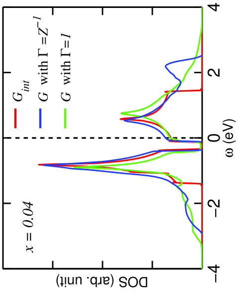
Figure 1: DOS computed from $G_{int}$ is compared with the fully dressed DOS with a vertex correction $\Gamma=1/Z$ and without the vertex correction (i.e. $\Gamma=1$) at a representative doping of $x$=0.04 as discussed in the text.

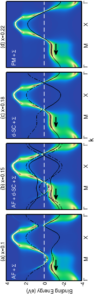
Figure 2: Spectral intensity plots along the high symmetry lines for antiferromagnetic (AF) ($x=0.10$), AF+$d-$wave superconducting (SC) ($x=0.15$), $d-$SC ($x=0.18)$, and the paramagnetic (PM) ($x=0.22$) states. Full self-energy $\Sigma$ is included in all cases. Antiferromagnetic order parameters are computed self-consistently.tanmoysw Self-energy is computed including the antiferromagnetic gap, but does not incorporate the low energy superconducting gap. Black lines depict the dispersions that enter into $G_{int}$, but the corresponding spectral weight of the band is not shown for simplicitykusko . An artificially large value of superconducting gap ($\Delta=30$ meV) is used so that the effects of superconductivity can be visible on the energy scale of the figure.tanmoyprb Arrows mark the start of the high-energy kink or the waterfall in the spectrum below the Fermi energy.

Self-consistency is obtained by choosing $Z$ such that the low energy dispersion is the same for $G$ and $G_{int}$. This is illustrated in Figs. 1 and 2. Fig. 1 compares the density-of-states (DOS) associated with $G_{int}$ (red line) and $G$, either with (blue line) or without (green) a vertex correction in the antiferromagnetic state. As discussed further below, $G$ and $G_{int}-$dressed DOSs clearly match well with each other in the low energy regime where both spectra show the spin density wave dressed upper and lower magnetic bands, consistent with our earlier mean-field resultskusko ; tanmoyprb ; tanmoyprl . At high energies, however, $G_{int}$ fails (by construction) to reproduce the incoherent hump features associated with precursors to the upper and lower Hubbard bands.

Fig. 2 compares the spectral weights, $A=-Im(G)/\pi$, with the corresponding dispersions $\epsilon_{{\bf k},int}$ (black lines) that enter into $G_{int}$. As noted earlier, the latter provide a very good fit to the low energy coherent features for the entire doping range in electron doped Nd_2-xCe_xCuO₄ (NCCO). Self-consistency ensures that $G_{int}$ provides the best approximation to the full $G$. As an added benefit, $Z$ in general renormalizes $\epsilon_{{\bf k},int}$ to values close to those found in our earlier mean-field studieskusko ; tanmoyprb ; tanmoyprl . The obtained self-consistent values of $Z$ decrease almost linearly with doping, as seen in ARPESsahrakorpiprb . In this way, the QP-GW model reproduces the results of our earlier mean-field calculations in the low energy region, while revealing new physics at higher energies [e.g., the waterfall effect].

We now comment on some applications of the present QP-GW model. The waterfall physics seen in ARPES spectra of the cuprates is a direct consequence of the self-energy correction, which introduces a peak in scattering at intermediate energies below as well as above the Fermi level as seen in Fig. 2.susmita This scattering splits the spectrum into a low-energy coherent part and a high-energy incoherent region. While the near-Fermi-level dispersion changes substantially as the magnetic and the superconducting phases evolve with doping, the overall energy regime of the waterfall phenomenon remains fairly doping independent (marked by arrows in Fig. 2), consistent with experiments.graf In the pseudogap region ($x=0.10$, Fig. 2(a)), the resulting ‘four band’-like structure (two magnetic bands and the two Hubbard bands) agrees well with clustergrober and quantum Monte Carlo calculationsjarrell . Near optimal doping $d-$wave superconductivity coexists with the antiferromagnetic state in a uniform phasetanmoyprb ; tanmoyprl resulting in further splitting of the coherent bands as seen in Fig. 2(b). The coherent bands approach the Fermi level with increasing spectral weight as the pseudogap collapses at a quantum critical doping near $x=0.17$ in both the electron and hole doped casetanmoy2gap . On the other hand, the Hubbard bands move towards higher energy as the doping increases and the spectral weight associated with these bands decreases, consistent with optical spectra.uchida ; onose

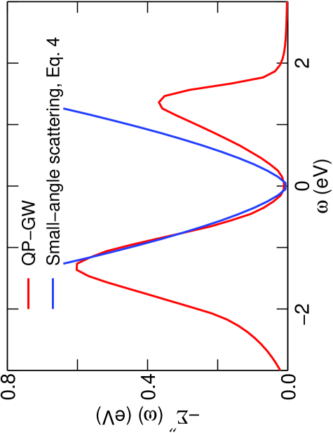
Figure 3: Imaginary part of the self-energy for NCCO (red line) is compared with the form used in Eq. 4. Note that the model small angle scattering formula was only applied to filled states, $\omega<0$.

Notably, the lifetime broadening of the quasiparticle states originates from magnetic scattering in the QP-GW model. This broadening has a non-Fermi liquid form with a significant linear-in-T component, particularly near the Van Hove singularity (VHS).markiewater Furthermore, in describing broadening of ARPES features in the superconducting state in our earlier mean-field model, we phenomenologically introduced an elastic small angle scattering contribution of similar non-Fermi-liquid formtanmoyprb ; hlubina ; dahm

$$\Sigma^{\prime\prime}(\omega)=sgn(\omega)C_{0}\left[1+\left(\frac{\omega}{\omega_{0}}\right)^{p}\right].$$ (4)

Here $C_{0}=100$ meV and $\omega_{0}=1.6$ eV are determined from a fit to the ARPES energy distribution curves (EDCs). The exponent $p$ is of physical significance in determining quasiparticle characterVidhyadhiraja . We found that $p=3/2$tanmoyprb ; hlubina ; dahm applies for electrons as well as hole doped cuprates in reproducing the ARPES spectra and quasiparticle interference (QPI) pattern seen in scanning tunneling spectroscopy. This scattering is particularly important in that it allows a finite spectral weight near the Fermi level even in the presence of a pseudogap, thereby revealing the leading edge superconducting gap at all momentatanmoyprb ; tanmoy2gap . In Fig. 3 we show that the imaginary part of the self-energy computed from Eq. 1 above reproduces this phenomenological form very well in the low-energy region, both in magnitude and $T$-dependence, indicating that magnon scattering underlies the anomalous exponent $p=3/2$.

We emphasize that in our QP-GW model the bare dispersion is taken directly from LDA, and the self-consistently determined $Z$ renormalizes this into a dispersion which matches the bands seen in ARPES experiments. Hence, the model reproduces our earlier mean-field results, but with fewer parameters, since the dispersion is calculated self-consistently rather than being derived from experiment.

As noted above, the high energy features are absent in $G_{int}$. This is also clear from Eq. 3: If we integrate the spectral weight $A_{int}({\bf k},\omega)$ over all frequencies we get $Z$, not $1$, so that $G_{int}$ accounts for only the coherent part of $G$. The incoherent part of weight, $1-Z$, is thus not accounted for. Clearly, this could be done straightforwardly by including a pair of broadened Lorentzians, but this will add additional parameters in the computation of the self-energy, not to mention associated vertex corrections. Therefore, we have chosen to first explore the QP-GW model without these complications. This is also the reason for calling our approach as QP-GW because it focuses on the QP part of the spectrum in evaluating $G_{int}$.

In order to better understand the susceptibility $\chi_{int}$, a comparison with our earlier mean-field result, $\chi_{MF}$ is instructive. Since $G_{int}$ differs from $G_{MF}$ only by an overall multiplicative factor of $Z$, $\chi_{int}$ differs from $\chi_{MF}$ by a factor of $Z^{2}$. This has important consequences. Fermi liquid theory requires that both the dispersion and the spectral weight be renormalized by interactions, and for a weakly $k$-dependent self energy, as in the present case, $Z_{disp}\simeq Z_{\omega}$. This is true for $G_{int}$ and $G$, but $Z_{\omega}=1$ for $G_{MF}$, which causes mean-field theory to overestimate the tendency towards instability. As the bandwidth decreases ($Z\rightarrow 0$), the density of states and susceptibility must increase as $1/Z$, in order to keep the total electron number fixed since there are no incoherent states in mean-field theory. Instability is controlled by the Stoner factor, $U\chi_{0}({\bf q},\omega=0)=1$. Since $\chi_{0}({\bf q},0,MF)=\chi_{0}({\bf q},0,LDA)/Z$, a small $Z$ enhances the probability of instability. On the other hand, for $G$ or $G_{int}$ only the low-energy quasiparticle degrees of freedom contribute to the instability, as reflected in $\chi_{0}({\bf q},0,int)=Z\chi_{0}({\bf q},0,LDA)$. Hence, large fluctuations (small $Z$) actually reduce the probability of condensing into any one mode. Equivalently, if we rewrite the Stoner factor in terms of the LDA susceptibility, it becomes $U_{eff}\chi_{0,LDA}=1$, with $U_{eff}=ZU$. Thus $t$ and $U$ should both be renormalized by factors of $Z$, leaving $t/U$ invariant. In our mean-field treatment, we had to assume that the effective $U$ was doping-dependent, and this $Z$-correction accounts for part of that doping dependence. .

It should be noted that an accurate calculation of the susceptibility and the resulting self-energy is fairly computer intensive as it involves a three-dimensional integral ($k_{x},k_{y},\omega$) for $\chi_{0}$ and a similar three-dimensional integral over $\chi$’s for $\Sigma$. Fortunately, we find that $\Sigma$ has only a weak $k$-dependence, so we need to calculate it only over a few $k$-points and use the average. Clearly, this is not a limitation of the model, and the full $k$-dependence could be calculated. However, this would make accurate self-consistent calculations substantially more time intensive. We have explored the use of a vertex correction for $\Sigma$, but the results are not too sensitive. We have typically taken $\Gamma=1/Z$, which puts somewhat greater weight into the incoherent bands as seen by comparing blue and green curves at higher energies in Fig. 2.

The present scheme can straightforwardly incorporate the full $k$-dependence of the susceptibility based on a realistic material specific band structure.Gzm1 This is important for delineating the nature of competing ordered phases, which are different for electron and hole doped cuprates. Moreover, our self-energy provides a tangible basis for going beyond the conventional LDA-based framework for realistic modeling of various highly resolved spectroscopies, providing more discriminating tests of theoretical models. In addition to the ARPES spectra discussed above, a note should also be made in this connection of the optical spectroscopy,tanmoysw STM tanmoytwogap ; Jouko ; joukoprb , RIXSsusmitarixs ; RIXS , x-ray absortion spectroscopy (XAS)towfiq and other inelastic light scattering spectroscopiesTanaka ; Huotari ; Barbiellini ; bansil to help piece together a robust understanding of the nature of electronic states in the cuprates and their evolution with doping.

In summary, we have shown that our intermediate coupling model of self-energy, which is based on the spin-wave dressing of the quasiparticles, can explain many anomalous features of the cuprates. At low energies, the model reproduces our mean field results for the coherent bands in ARPES,susmita optical,tanmoysw and RIXS,susmitarixs with self-energy corrections renormalizing the large widths of the LDA dispersions. At high energies, we obtain the waterfall features which represent a splitting off of the incoherent bands, precursors of the Mott gaps seen in ARPES and optical studies. In the underdoped regime, the coherent in-gap bands reproduce both the four-band behavior seen in quantum cluster calculations and the magnetic gap collapse found in the mean-field calculations and a variety of experiments. These results clearly suggest that the cuprates can be understood within the intermediate coupling regime with an effective $U$ value substantially smaller than twice the bandwidth.

- (1) N. Doiron-Leyraud, C. Proust, D. LeBoeuf, J. Levallois, J.-B. Bonnemaison, R. Liang, D. A. Bonn, W. N. Hardy, and L. Taillefer, Nature (London) 447, 565 (2007).
- (2) N. E. Hussey, M. Abdel-Jawad, A. Carrington, A. P. Mackenzie, L. Balicas, Nature 425, 814 (2003).
- (3) A.D. Beyer, M.S. Grinolds, M.L. Teague, S. Tajima, and N.-C. Yeh, arXiv:0808.3016, accepted for publication in Europhysics Letters.
- (4) L.F. Tocchio, F. Becca, A. Parola, and S. Sorella, Phys. Rev. B 78, 041101 (2008).
- (5) A. Comanac, L de Medici, M. Capone, and A. J. Millis, Nature Physics, 4, 287 (2008).
- (6) Tanmoy Das, R. S. Markiewicz and A. Bansil, arXiv:0807.4257.
- (7) K.-Y. Yang, T.M. Rice, and F.-C. Zhang, Phys. Rev. B 73, 174501 (2006).
- (8) A. Paramekanti, M. Randeria, and N. Trivedi, Phys. Rev. B 70, 054504 (2004).
- (9) R. S. Markiewicz, S. Sahrakorpi, and A. Bansil, Phys. Rev. B 76, 174514 (2007).
- (10) Tanmoy Das, R. S. Markiewicz, and A. Bansil, Phys. Rev. B 77, 134516 (2008) .
- (11) R.S. Markiewicz, J. Lorenzana, G. Seibold, and A. Bansil, unpublished.
- (12) Tanmoy Das, R.S. Markiewicz and A. Bansil, J. Phys. Chem. Solids, 69, 2963 (2008).
- (13) N.P. Armitage, D.H. Lu, C. Kim, A. Damascelli, K.M. Shen, F. Ronning, D.L. Feng, H. Eisaki, Z.-X. Shen, P.K. Mang, N. Kaneko, M. Greven, Y. Onose, Y. Taguchi, and Y. Tokura, Phys. Rev. Lett. 88, 257001 (2002).
- (14) C. Kusko, , R. S. Markiewicz, M. Lindroos, and A. Bansil, Phys. Rev. B. 66, 140513(R) (2002).
- (15) R.S. Markiewicz and A. Bansil, Phys. Rev. Lett. 96, 107005 (2006).
- (16) Tanmoy Das, R.S. Markiewicz, and A. Bansil, Phys. Rev. B 77, 134516 (2008).
- (17) Tanmoy Das, R. S. Markiewicz and A. Bansil, Phys. Rev. Lett. 98, 197004 (2007).
- (18) T. Helm, M.V. Kartsovnik, M. Bartkowiak, N. Bittner, M. Lambacher, A. Erb, J. Wosnitza, and R. Gross, Phys. Rev. Lett. 103, 157002 (2009).
- (19) R.S. Markiewicz, Phys. Rev. B 70, 174518 (2004).
- (20) F. Ronning, K. M. Shen, N. P. Armitage, A. Damascelli, D. H. Lu, Z.-X. Shen, L. L. Miller, and C. Kim, Phys. Rev. B 71, 094518 (2005).
- (21) J. Graf, G.-H. Gweon, K. McElroy, S. Y. Zhou, C. Jozwiak, E. Rotenberg, A. Bill, T. Sasagawa, H. Eisaki, S. Uchida, H. Takagi, D.-H. Lee, and A. Lanzara, Phys. Rev. Lett. 98, 067004 (2007).
- (22) Z.-H. Pan, P. Richard, A.V. Fedorov, T. Kondo, T. Takeuchi, S.L. Li, Pengcheng Dai, G.D. Gu, W. Ku, Z. Wang, H. Ding, arXiv:0610442v2.
- (23) M. Lindroos, S. Sahrakorpi, and A. Bansil, Phys. Rev. B 65, 054514 (2002).
- (24) M. C. Asensio, J. Avila, L. Roca, A. Tejeda, G. D. Gu, M. Lindroos, R. S. Markiewicz, and A. Bansil, Phys. Rev. B 67, 014519 (2003).
- (25) A. Bansil, M. Lindroos, S. Sahrakorpi, and R. S. Markiewicz, Phys. Rev. B 71, 012503 (2005).
- (26) S. Sahrakorpi, M. Lindroos, R. S. Markiewicz, and A. Bansil, Phys. Rev. Lett. 95, 157601 (2005).
- (27) Susmita Basak, Tanmoy Das, Hsin Lin, J. Nieminen, M. Lindroos, R.S. Markiewicz, A. Bansil, Phys. Rev. B 80, 214520 (2009).
- (28) Y. Onose, Y. Taguchi, , K. Ishizaka, and Y. Tokura, Phys. Rev. Lett. 87, 217001 (2001).
- (29) Y. Onose, Y. Taguchi, K. Ishizaka, Y. Tokura, Phys. Rev. B 69, 024504 (2004).
- (30) S. Uchida, T. Ido, H. Takagi, T. Arima, Y. Tokura and S. Tajima Phys. Rev. B 43, 7942 (1991).
- (31) G. Vignale and M. R. Hedayati, Phys. Rev. B 42, 786 (1990).
- (32) The self energy is calculated in Matsubara space and continued analytically as where is a positive infinitesimal.
- (33) Giovanni Onida, Lucia Reining, and Angel Rubio, Rev. Mod. Phys. 74, 601 (2002).
- (34) R.S. Markiewicz, S. Sahrakorpi, M. Lindroos, Hsin Lin, and A. Bansil, Phys. Rev. B 72, 054519 (2005).
- (35) Tanmoy Das, R.S. Markiewicz, and A. Bansil, Phys. Rev. B 74, 020506(R) (2006).
- (36) S. Sahrakorpi, R. S. Markiewicz, Hsin Lin, M. Lindroos, X. J. Zhou, T. Yoshida, W. L. Yang, T. Kakeshita, H. Eisaki, S. Uchida, Seiki Komiya, Yoichi Ando, F. Zhou, Z. X. Zhao, T. Sasagawa, A. Fujimori, Z. Hussain, Z.-X. Shen, and A. Bansil, Phys. Rev. B 78, 104513 (2008).
- (37) C. Gröber, R. Eder, and W. Hanke, Phys. Rev. B 62, 4336 (2000).
- (38) M. Jarrell, Th. Maier , M. H. Hettler, A. N. Tahvildarzadeh, Europhysics Letter, 56, 563 (2001).
- (39) R. Hlubina and T. M. Rice, Phys. Rev. B 51, 9253 (1995); R. S. Markiewicz, Phys. Rev. B 69, 214517 (2004).
- (40) T. Dahm, P. J. Hirschfeld, L. Zhu, and D. J. Scalapino, Phys. Rev. B 71, 212501 (2005).
- (41) N. S. Vidhyadhiraja, A. Macridin, C. Sen, M. Jarrell, and Michael Ma, Phys. Rev. Lett. 102, 206407 (2009).
- (42) J. Nieminen, Hsin Lin, R. S. Markiewicz, and A. Bansil, Phys. Rev. Lett. 102, 037001 (2009).
- (43) Jouko Nieminen, Ilpo Suominen, R. S. Markiewicz, Hsin Lin, and A. Bansil, accepted in Phys. Rev. B (2009).
- (44) Susmita Basak, Tanmoy Das, Hsin Lin, R. S. Markiewicz, and A. Bansil, Manuscript under preparation, APS March Meeting Abstract: Q41.00007 (2010).
- (45) Towfiq Ahmed, John J. Rehr, Joshua J. Kas, Tanmoy Das, Hsin Lin, R. S. Markiewicz, B. Barbiellini, and A. Bansil, Manuscript under preparation, APS March Meeting Abstract: Z40.00012 (2010).
- (46) Yoshikazu Tanaka, Y. Sakurai, A. T. Stewart, N. Shiotani, P. E. Mijnarends, S. Kaprzyk, and A. Bansil, Phys. Rev. B 63, 045120 (2001).
- (47) S. Huotari, K. Hmlinen, S. Manninen, S. Kaprzyk, A. Bansil, W. Caliebe, T. Buslaps, V. Honkimki, and P. Suortti, Phys. Rev. B 62, 7956 (2000).
- (48) B. Barbiellini, A. Koizumi, P. E. Mijnarends, W. Al-Sawai, Hsin Lin, T. Nagao, K. Hirota, M. Itou, Y. Sakurai, and A. Bansil, Phys. Rev. Lett. 102, 206402 (2009).