Chaotic Maps, Hamiltonian Flows, and Holographic Methods

Abstract

Holographic functional methods are introduced as probes of discrete time-stepped maps that lead to chaotic behavior.  The methods provide continuous time interpolation between the time steps, thereby revealing the maps to be quasi-Hamiltonian systems underlain by novel potentials that govern the motion of a perceived point particle.  Between turning points, the particle is strictly driven by Hamiltonian dynamics, but at each encounter with a turning point the potential changes abruptly, loosely analogous to the switchbacks on a mountain road.  A sequence of successively deepening switchback potentials explains, in physical terms, the frequency cascade and trajectory folding that occur on the particular route to chaos revealed by the logistic map.

year number number identifier LABEL:FirstPage1 LABEL:LastPage#1

I Introduction

In a previous paper CZ  we have discussed how functions of position, defined on a discrete lattice of time points, may be analytically interpolated in time by functions of both $x$ and $t$, defined on a continuum of time points, framed by the lattice, through the use of solutions to Schröder’s nonlinear functional equation S .  For a more pedagogical discussion to augment this Introduction, we encourage readers to look at that companion paper.

If the effect of the first discrete time step is given as the map $x\mapsto f_{1}\left(x,s\right)$, for some parameter $s$, Schröder’s functional equation is

$$s\Psi\left(x,s\right)=\Psi\left(f_{1}\left(x,s\right),s\right)\ ,$$ (1)

with $\Psi$ to be determined.  So,

$$f_{1}\left(x,s\right)=\Psi^{-1}\left(s\Psi\left(x,s\right),s\right)\ ,$$ (2)

where the inverse function $\Psi^{-1}$ obeys Poincaré’s equation,

$$\Psi^{-1}\left(sx,s\right)=f_{1}\left(\Psi^{-1}\left(x,s\right),s\right)\ .$$ (3)

The $n$th iterate of (1) gives

$$s^{n}\Psi\left(x,s\right)=\Psi\left(f_{1}\left(\cdots f_{1}\left(f_{1}\left(x,s\right),s\right)\cdots,s\right),s\right)\ ,$$ (4)

with $f_{1}$ acting $n$ times, and thus the $n$th order functional composition — the so-called “splinter” of the functional equation —

$$f_{n}\left(x,s\right)\equiv f_{1}\left(\cdots f_{1}\left(f_{1}\left(x,s\right),s\right)\cdots,s\right)=\Psi^{-1}\left(s^{n}\Psi\left(x,s\right),s\right)\ .$$ (5)

A continuous interpolation between the integer lattice of time points is then, for any $t$,

$$f_{t}\left(x,s\right)=\Psi^{-1}\left(s^{t}\Psi\left(x,s\right),s\right)\ .$$ (6)

This can be a well-behaved and single-valued function of $x$ and $t$ provided that $\Psi^{-1}\left(x,s\right)$ is a well-behaved, single-valued function of $x$, even though $\Psi\left(x,s\right)$ might be, and typically is, multi-valued.

As discussed in CZ , the interpolation can be envisioned as the trajectory of a particle,

$$x\left(t\right)=f_{t}\left(x,s\right)\ ,$$ (7)

where the particle is moving under the influence of a potential according to Hamiltonian dynamics.  The velocity of the particle is then found by differentiating (6) with respect to $t$,

$$\frac{dx\left(t\right)}{dt}=\left(\ln s\right)s^{t}\Psi\left(x\right)\left(\Psi^{-1}\left(s^{t}\Psi\left(x\right)\right)\right)^{\prime}\ ,$$ (8)

where any dependence of $\Psi$ on $s$ is implicitly understood.  Therefore, the velocity will inherit and exhibit any multi-valuedness possessed by $\Psi\left(x\right)$.

Indeed, suppose that Hamiltonian dynamics have been specified, trajectories have been computed, and $f_{1}=x\left(t=1\right)$ has emerged in terms of initial velocity and initial position $x\left(t=0\right)\equiv x$.  A solution of the functional equation (1) can then be constructed, and expressed in very physical terms, as just an exponential of the time elapsed along any such particle trajectory that passes through position $x$.  That solution is

$$\Psi\left(x\right)=s^{T\left(x\right)}\Psi_{0}\ ,\ \ \ T\left(x\right)=\int^{x}\frac{dy}{v\left(y\right)}\ .$$ (9)

Here $v$ is the velocity as a function of the position along the trajectory.  (Hence $v\left(x\left(t\right)\right)$, if you wish.  Of course, for a Hamiltonian system with time translational invariance, we may supplant $x\left(t\right)\rightarrow x\left(t+\Delta t\right)$ in all these expressions, as well as those to follow.)  For a particle moving in a potential $V\left(x\right)$ at fixed energy, $E$, the velocity can be expressed in the usual way as $v\left(x\right)=\pm\sqrt{E-V\left(x\right)}$, with suitably chosen mass units.

When written in a form more closely related to Schröder’s functional equation, the solution (9) is simply

$$\Psi\left(f_{t}\left(x\right)\right)=s^{\int_{x}^{f_{t}\left(x\right)}\frac{dy}{v\left(y\right)}}~{}\Psi\left(x\right)\ .$$ (10)

At $t=1$, $\int_{x}^{f_{1}\left(x\right)}\frac{dy}{v\left(y\right)}=1$, and Schröder’s equation (1) re-emerges.  But, as this construction clearly shows, one must be careful at turning points where $v=0$, especially if these are encountered at finite times along the trajectory.  Typically these turning points produce branch points in $\Psi$ so that it is multi-valued.

An interesting physical effect of such branch points, when they are encountered in finite times, is the possibility to switch from one branch of the underlying analytic potential function to another, thereby changing the functional form of the Hamiltonian governing the motion along seemingly identical intervals of a real-valued trajectory.  We will therefore call these quasi-Hamiltonian systems, and we stress that when such switches occur this is not standard textbook Hamiltonian dynamics.  Further explanation will be given below in the context of the logistic map.

The interpolation (6) can also be viewed as a holographic specification on the $x,t$ plane L , determining $f_{t}\left(x\right)$ in the surrounded “bulk” from the total data given at the bounding times, $\left\{x\right\}\cup\left\{f_{1}\left(x\right)\right\}$.  In this point of view, fixed points in $x$ complete the boundary data and facilitate the solution of Schröder’s equation through power series in $x$, hence leading to $V\left(x\right)$ which was not known a priori CZ .

In this holographic approach, the potential first appears as a quadratic in $\Psi/\Psi^{\prime}$,

$$V\left(x\right)=-\left(\ln s\right)^{2}\left(\frac{\Psi\left(x\right)}{\Psi^{\prime}\left(x\right)}\right)^{2}\ ,$$ (11)

up to an additive constant, where any dependence of $\Psi$ on $s$ is again implicit.  The $x$ dependence of the potential,

$$V\left(x\right)\equiv-v^{2}\left(x\right)\ ,$$ (12)

follows from that of the velocity profile of the interpolation, defined and given by LogicalConnections

$$v\left(x\right)\equiv\left.\frac{df_{t}\left(x\right)}{dt}\right|_{t=0}=\left(\ln s\right)\Psi\left(x\right)\left(\Psi^{-1}\left(\Psi\left(x\right)\right)\right)^{\prime}=\frac{\ln s}{\frac{d}{dx}\ln\Psi\left(x\right)}\ .$$ (13)

Monotonic motions between two fixed points, such as occur for the Ricker model R , provide the most elementary examples CZ .

However, situations where one or both of the fixed points are absent were not fully addressed in our previous work.  This is precisely the situation that occurs when turning points are encountered at finite times in the particle dynamics interpretation, and leads to an intriguing modification in the physical picture involving the potential and its effect on the particle trajectories.  We consider here a specific example of such a situation involving the well-studied logistic map of chaotic dynamics, namely M ; CE ; F ; K ; C ,

$$x\mapsto sx\left(1-x\right)\ .$$ (14)

Applying our functional methods to this example, the resulting interpolations from a discrete lattice of time points to a time continuum then allow us to appreciate analytic features of the logistic map, and to derive the governing differential evolution laws — indeed, subtly time-translation-invariant Hamiltonian dynamical laws — of the underlying physical system, hence to obtain potentials that were not previously known.

For the all-familiar logistic map illustrating transition to chaos, the functional interpolation reveals that there are well-defined expressions for the continuous time evolution of this map for all parametric values of the map, whether chaotic or not.  We obtain agreement with the explicit closed-form solutions of (1) for the special values of the parameters: $s=-2,\ 2,$ and $4$.  (These explicit solutions have been known for almost a century and a half S .)   Moreover, as indicated, from (11) we can now find the potentials needed to produce these explicit, continuously evolving trajectories in the language of Hamiltonian dynamics.

A new feature for the potentials so obtained for the $s=4$ case in particular, and also for other values of $s>2$, is that they must change at discrete intervals of the envisioned Hamiltonian particle’s motion, to be consistent with the evolution trajectories:  Every time the particle hits a turning point, the potential changes Footnote1 .  We therefore call the corresponding $V$s “switchback potentials” and to echo our previous general remarks, we will call the dynamical system as a whole “quasi-Hamiltonian.”  For $s=4$ the switchback potentials deepen successively and thus lead to more rapid, higher frequency motion, resulting in the familiar chaotic behavior of the discrete $s=4$ logistic map that they interpolate.  The familiar frequency-cascade-and-folding behavior of the chaotic discrete map is thus understood from — indeed, explained by — the subtle properties of the switchback potentials.

II The Logistic Map

Consider in detail the logistic map (14) on the unit interval, $x\in\left[0,1\right]$.  Schröder’s equation for this map is

$$s\Psi\left(x,s\right)=\Psi\left(sx\left(1-x\right),s\right)\ .$$ (15)

The inverse function satisfies the corresponding Poincaré equation,

$$\Psi^{-1}\left(sx,s\right)=s\Psi^{-1}\left(x,s\right)\left(1-\Psi^{-1}\left(x,s\right)\right)\ .$$ (16)

As originally obtained by Schröder, there are three closed-form solutions known, for $s=-2,$ $2,$ and $4$:

$$\Psi\left(x,-2\right) =\frac{\sqrt{3}}{6}\left(2\pi-3\arccos\left(x-\frac{1}{2}\right)\right)\ ,\ \ \ \Psi^{-1}\left(x,-2\right)=\frac{1}{2}-\cos\left(\frac{2x}{\sqrt{3}}+\frac{\pi}{3}\right)\ ,$$

$$\Psi\left(x,2\right) =-\frac{1}{2}\ln\left(1-2x\right)\ ,\ \ \ \Psi^{-1}\left(x,2\right)=\frac{1}{2}\left(1-e^{-2x}\right)\ ,$$

$$\Psi\left(x,4\right) =\left(\arcsin\sqrt{x}\right)^{2}\ ,\ \ \ \Psi^{-1}\left(x,4\right)=\left(\sin\sqrt{x}\right)^{2}\ .$$ (17)

Note that, while the $\Psi$ are multi-valued, the inverse functions are all single-valued.

More generally, consider a power series for any $s$.

$$\Psi^{-1}\left(x,s\right)=x+x\sum_{n=1}^{\infty}x^{n}c_{n}\left(s\right)\ .$$ (18)

The Poincaré equation then leads to a recursion relation for the $s$-dependent coefficients.

$$c_{n+1}=\frac{1}{1-s^{n+1}}\sum_{j=0}^{n}c_{j}c_{n-j}\ ,$$ (19)

with $c_{0}=1$, $c_{1}=\frac{1}{1-s}$, $c_{2}=\frac{2}{\left(1-s\right)\left(1-s^{2}\right)}$, etc.  The explicit coefficients are easily recognized for $s=-2,$ $2,$ and $4$, and immediately yield the three closed-form cases.  Similarly let

$$\Psi\left(x,s\right)=x+x\sum_{n=1}^{\infty}\left(-x\right)^{n}d_{n}\left(s\right)\ .$$ (20)

Then, as a consequence of Schröder’s equation, $d_{1}=1/\left(1-s\right)$, and for $n\geq 2$,

$$d_{n}=\frac{1}{1-s^{n}}\sum_{k=1}^{\left\lfloor\frac{n+1}{2}\right\rfloor}\binom{n+1-k}{k}s^{n-k}d_{n-k}\ .$$ (21)

where $\left\lfloor\cdots\right\rfloor$ is the (integer-valued) floor function.  In principle, these series solve (16) and (15) for any $s$, within their radii of convergence.

From extensive numerical studies we believe the radius of convergence for (20) depends on $s$ as follows.

$$R_{\Psi}=\left\{\begin{array}[c]{ccc}\left|1-\dfrac{1}{s}\right|&\text{if}&0\leq s\leq 2\ ,\\ &&\\ \dfrac{s}{4}&\text{if}&2\leq s\leq 4\ .\end{array}\right.$$ (22)

Preliminary work further suggests that these conjectural results can actually be established analytically by comparison with known convergent series, at least in some cases.

The radius of convergence for the inverse function series (18) is intriguing for $0\leq s\leq 1$.  A fit by Mathematica to radii obtained numerically from explicit series coefficients $c_{n}\left(s\right)$ up to $n=200$, for 20 different values of $s$ in this range, using the functional form $\frac{1}{4}\left(1-s\right)^{a}\exp bs$, gives $a=0.78$ and $b=0.62$.  Thus $R_{\Psi^{-1}}\left(s\right)$ falls from $1/4$ to zero as $s$ goes from $0$ to $1$.  However, for the parameters of most interest, namely $2\leq s\leq 4$, numerical studies suggest the series all have infinite radius of convergence, indicating the $\Psi^{-1}$ are entire functions for these parameters.  This is true for $s=2$ and $s=4$, of course, as is evident from (17).  The numerics provide compelling evidence that this is also true for all intermediate $s$.

Given convergent series, the functional equations can then be used to continue the series solutions outside their radii of convergence and thereby obtain accurate determinations of the various branches of $\Psi$, and of the large-but-finite argument behavior of $\Psi^{-1}$, in a manner familiar from, say, the $\Gamma$ and $\zeta$ functions.  (See CV  for details, and the Appendix for a numerical example.)  Comparison of the results from these series-plus-functional-equation methods with the known exact solutions (17) shows perfect agreement.

The first few terms for $\Psi$ and $\Psi^{-1}$ for generic $s$ are given explicitly by s=0

$$\Psi\left(x,s\right)=x+\frac{x^{2}}{s-1}+\frac{2s}{\left(s+1\right)}\frac{x^{3}}{\left(s-1\right)^{2}}+\frac{s\left(1+5s^{2}\right)}{\left(s^{2}+s+1\right)\left(s+1\right)}\frac{x^{4}}{\left(s-1\right)^{3}}$$

$$+\frac{2s^{3}\left(3+2s+7s^{3}\right)}{\left(s^{2}+1\right)\left(s^{2}+s+1\right)\left(s+1\right)^{2}}\frac{x^{5}}{\left(s-1\right)^{4}}$$

$$+\frac{2s^{3}\left(1+3s+14s^{3}+14s^{4}+7s^{5}+21s^{7}\right)}{\left(s^{4}+s^{3}+s^{2}+s+1\right)\left(s^{2}+1\right)\left(s^{2}+s+1\right)\left(s+1\right)^{2}}\frac{x^{6}}{\left(s-1\right)^{5}}+O\left(x^{7}\right)\ ,$$ (23)

$$\Psi^{-1}\left(x,s\right)=x+\frac{x^{2}}{1-s}+\frac{2}{\left(s+1\right)}\frac{x^{3}}{\left(s-1\right)^{2}}+\frac{5+s}{\left(s+1\right)\left(s^{2}+s+1\right)}\frac{x^{4}}{\left(1-s\right)^{3}}$$

$$+\frac{2\left(7+3s+2s^{2}\right)}{\left(s^{2}+1\right)\left(s^{2}+s+1\right)\left(s+1\right)^{2}}\frac{x^{5}}{\left(s-1\right)^{4}}$$

$$+\frac{2\left(21+14s+14s^{2}+8s^{3}+3s^{4}\right)}{\left(s^{4}+s^{3}+s^{2}+s+1\right)\left(s^{2}+1\right)\left(s^{2}+s+1\right)\left(s+1\right)^{2}}\frac{x^{6}}{\left(1-s\right)^{5}}+O\left(x^{7}\right)\ ,$$ (24)

from which we infer that $\Psi\left(x,s\right)/x$ and $\Psi^{-1}\left(x,s\right)/x$ are actually series in $x/\left(1-s\right)$ with $s$-dependent coefficients that are analytic near $s=1$.

The trajectories interpolating the splinter (integer $t$) of the logistic map are then,

$$x\left(t\right)=\Psi^{-1}\left(s^{t}\Psi\left(x,s\right),s\right)=s^{t}~{}x+\frac{s^{t}\left(1-s^{t}\right)}{s-1}~{}x^{2}+\frac{2s^{t}\left(1-s^{t}\right)\left(s-s^{t}\right)}{\left(s+1\right)\left(s-1\right)^{2}}~{}x^{3}$$

$$+\frac{s^{t}\left(1-s^{t}\right)\left(s-s^{t}\right)\left(1+5s^{2}-\left(s+5\right)s^{t}\right)}{\left(s+1\right)\left(s^{2}+s+1\right)\left(s-1\right)^{3}}~{}x^{4}$$

$$+\frac{2s^{t}\left(1-s^{t}\right)\left(s-s^{t}\right)\left(s^{2}-s^{t}\right)\left(7s^{3}+2s+3-s^{t}\left(2s^{2}+3s+7\right)\right)}{\left(s+1\right)^{2}\left(s^{2}+1\right)\left(s^{2}+s+1\right)\left(s-1\right)^{4}}~{}x^{5}+O\left(x^{6}\right)\ .$$ (25)

The trajectories are single-valued functions of the time so long as $\Psi^{-1}$ is single-valued, and in fact, they exist even for $s\rightarrow 1$ as formal series solutions.   Explicitly,

$$\lim\limits_{s\rightarrow 1}\Psi^{-1}\left(s^{t}\Psi\left(x,s\right),s\right)=x-t~{}x^{2}+t\left(t-1\right)~{}x^{3}-\frac{1}{2}t\left(t-1\right)\left(2t-3\right)~{}x^{4}$$

$$+\frac{1}{3}t\left(t-1\right)\left(t-2\right)\left(3t-4\right)~{}x^{5}-\frac{1}{12}t\left(t-1\right)\left(t-2\right)\left(12t^{2}-41t+31\right)~{}x^{6}$$

$$+\frac{1}{30}t\left(t-1\right)\left(t-2\right)\left(30t^{3}-171t^{2}+302t-157\right)~{}x^{7}+O\left(x^{8}\right)\ .$$ (26)

For the three special cases, $s=-2,\ 2,$ and $4$, there are closed-form results for various quantities of interest.  For example, for $s=4$, the trajectory and velocity are given by

$$\left.x\left(t\right)\right|_{s=4}=\Psi^{-1}\left(4^{t}~{}\Psi\left(x,4\right),4\right)=\left(\sin\left(2^{t}\arcsin\sqrt{x}\right)\right)^{2}\ ,$$ (27)

(as originally presented in S , p 306) and by

$$\frac{d}{dt}x\left(t\right) =\left(2^{1+t}\ln 2\right)\sin\left(2^{t}\arcsin\sqrt{x}\right)\cos\left(2^{t}\arcsin\sqrt{x}\right)\arcsin\sqrt{x}$$ (28a)

$$=\left(\ln 4\right)\sqrt{x\left(t\right)\left(1-x\left(t\right)\right)}\arcsin\sqrt{x\left(t\right)}\ .$$ (28b)

The last expression evinces a continuous time-translational invariance.  However, this velocity function has branch points (i.e. turning points) at $$x\left(t\right)=0 x\left(t\right)=1$$ and , so some care is needed to determine which branch of the function is involved, particularly when the turning points are encountered at finite times.  The system is therefore a quasi-Hamiltonian one, as we have previously indicated, and as we shall discuss in more detail.

With this caveat in mind, we may thus deduce the velocity profile $v\left(x\right)=\left.\frac{dx\left(t\right)}{dt}\right|_{t=0}$, the effective potential, and the force for the underlying quasi-Hamiltonian system:

$$v\left(x\right) =\left.\frac{dx\left(t\right)}{dt}\right|_{s=4,t=0}=\left(\ln 4\right)\sqrt{x\left(1-x\right)}\arcsin\sqrt{x}\ ,$$ (29)

$$V\left(x\right) =-v^{2}\left(x\right)=\left(\ln 4\right)^{2}x\left(x-1\right)\arcsin^{2}\sqrt{x}\ ,$$ (30)

$$F\left(x\right) =-\frac{d}{dx}V\left(x\right)=\left(\ln 4\right)^{2}\left(\arcsin\sqrt{x}\right)\left(\sqrt{x\left(1-x\right)}-\left(2x-1\right)\arcsin\sqrt{x}\right)\ .$$ (31)

Note $x=0$ is an unstable fixed point for the system.  Also, the system is time-translationally invariant, so these same expressions hold at all times everywhere along a trajectory, provided due care is taken to determine which branch of the various functions is in effect. Thus $V\left(x\left(t\right)\right)=\left(\ln 4\right)^{2}x\left(t\right)\left(x\left(t\right)-1\right)\arcsin^{2}\sqrt{x\left(t\right)}$, etc.

Similar closed-form results hold for the other two solvable cases, $s=-2$ and $s=2$.  In principle, there are also potentials underlying the trajectories for other $s$ by dint of the series constructions.  (We illustrate one other case, $s=3$, in the Appendix.)

From the general expression for $x\left(t\right)$ in terms of $\Psi$ and $\Psi^{-1}$, and with use of the chain rule, the potential may be expressed entirely in terms of $\left(\ln\Psi\right)^{\prime}$, as given in the Introduction by (11).  The Schröder auxiliary function is then recognized as just an exponential of the time function

$$T\left(x\right)=\int^{x}\frac{dy}{\sqrt{-V\left(y\right)}}\ ,$$ (32)

computed along a zero-energy trajectory, as given by (9).

III Novel potentials and switchback effects

The effective potentials for all three closed-form cases are somewhat unusual:

$$V\left(x,s=4\right) =\left(\ln 4\right)^{2}x\left(x-1\right)\arcsin^{2}\sqrt{x}\ ,$$ (33)

$$V\left(x,s=2\right) =-\left(\ln\sqrt{2}\right)^{2}\left(1-2x\right)^{2}\ln^{2}\left(1-2x\right)\ ,$$ (34)

$$V\left(x,s=-2\right) =\frac{1}{36}\left(\ln\left(-2\right)\right)^{2}\left(2x+1\right)\left(2x-3\right)\left(2\pi-3\arccos\left(x-\frac{1}{2}\right)\right)^{2}\ .$$ (35)

Another way to express the potential for $s=4$ is similar in form to that for $s=-2$, namely,

$$V\left(x,s=4\right)=\left(\ln 2\right)^{2}x\left(x-1\right)\left(\pi-\arccos\left(2x-1\right)\right)^{2}\ .$$ (36)

Indeed, it is well-known that the logistic maps for $s=4$ and $s=-2$ are intimately related through the functional conjugacy of the underlying Schröder equations.  But note the potential for $s=-2$ is in fact complex, since $\ln\left(-2\right)=\ln 2+i\pi$, as are the trajectories under real time evolution for this case.  Of course, since the complexity of $V\left(x,s=-2\right)$ is solely a multiplicative factor, if we switch to complex time, $\tau=\left(\ln 2+i\pi\right)\times t$, then

$$\frac{d^{2}x}{d\tau^{2}}=-\frac{\partial}{\partial x}\frac{V\left(x,s=-2\right)}{2\left(\ln 2+i\pi\right)^{2}}$$ (37)

again yields real trajectories $x\left(\tau\right)$.  As trivial as this observation is, nevertheless it does raise several questions about complex $x$, and about the behavior of $V$ in the complex plane.  We discuss only one aspect of this behavior here, and consider non-principal values for the multi-valued functions $v\left(x,s=4\right)$ and $V\left(x,s=4\right)$.  In particular, all branches of the $\arcsin$ function are important to understand the behavior of the explicit trajectories (27).

Switchbacks on the road to chaos.  An interesting new feature, which we shall call the switchback effect, appears for a particle moving in the $s=4$ effective potential.  This is a distinguishing feature that we encounter for the $s=4$ chaotic map, but not, say, for the non-chaotic $s=2$ map.  The effect is traceable to the fact that, while the trajectory is single-valued as a function of the time, the velocity and hence the effective potential are not single-valued as functions of position.  Moreover, the branch points of the multi-valued functions are encountered by zero-energy trajectories at finite times for the $s=4$ case, unlike, say, for the $s=2$ case.  For the latter case, it takes an infinite time for a particle with zero energy to reach a turning point.

Switchbacks are essentially transitions from one branch of the position-dependent velocity function to another, and occur at the turning points encountered at finite times by the interpolating particle trajectories, (27).  The effect is easily seen upon viewing animations of these trajectories Animations .

Consider a particle with zero total energy that starts in the $V\left(x,s=4\right)$ potential given above, in the region $0<x<1$.  If the particle is initially moving to the left, it will continue towards $x=0$, taking an infinite amount of time to reach that turning point.  But if the particle is initially moving to the right, it will reach the $x=1$ turning point in a finite amount of time that depends on its initial $x$, as given by

$$\Delta t_{0}\left(x\right)=\frac{1}{\ln 4}\int_{x}^{1}\frac{dy}{\sqrt{y\left(1-y\right)}\left(\arcsin\sqrt{y}\right)}=\frac{1}{\ln 2}~{}\ln\left(\frac{\pi/2}{\arcsin\sqrt{x}}\right)\ .$$ (38)

So, for example, starting from the midpoint $x=1/2$, it takes unit time to reach the turning point at $x=1$.

Upon reaching $x=1$, the explicit form of the time-dependent solution (27) exhibits the classical counterpart of a sudden transition that keeps $E=0$, but changes the potential for the return trip towards $x=0$, exactly as follows from the particle moving on a different branch of the $\arcsin$ function.  Explicitly, the potential deepens to

$$V\left(x,s=4\right)\Longrightarrow V_{1}\left(x\right)=\left(\ln 4\right)^{2}x\left(x-1\right)\left(-\pi+\arcsin\sqrt{x}\right)^{2}\ ,$$ (39)

with the particle’s speed changing accordingly as a function of $x$.   The return velocity profile is now negative, and given by

$$v_{1}\left(x\right)=\left(\ln 4\right)\sqrt{x\left(1-x\right)}\left(-\pi+\arcsin\sqrt{x}\right)\ .$$ (40)

The $\arcsin$ in this last expression, as well as in $V_{1}$, is understood to be the principal value.

Moving in this modified negative potential, it now takes the zero-energy particle a finite amount of time to travel from $x=1$ down to $x=0$, as given by $\Delta t_{1}=1$.  Upon reaching $x=0$, the exact solution (27) exhibits another sudden transition that keeps $E=0$, but again alters the potential for the return trip towards $x=1$.  The potential becomes

$$V_{1}\left(x\right)\Longrightarrow V_{2}\left(x\right)=\left(\ln 4\right)^{2}x\left(x-1\right)\left(\pi+\arcsin\sqrt{x}\right)^{2}\ ,$$ (41)

with corresponding changes in the velocity profile.  Again, a finite amount of time is needed for the particle to go from $x=0$ to $x=1$ in the potential $V_{2}$, as given by $\Delta t_{2}=\ln\left(\frac{3}{2}\right)/\ln 2$.

Upon reaching $x=1$ again, the switchback process continues.  The total energy remains at zero, but the potential for the second return trip further deepens,

$$V_{2}\left(x\right)\Longrightarrow V_{3}\left(x\right)=\left(\ln 4\right)^{2}x\left(x-1\right)\left(-2\pi+\arcsin\sqrt{x}\right)^{2}\ ,$$ (42)

etc.  In order for the particle to follow the interpolating trajectory (27) specified by the Schröder equation for the $s=4$ case, it has to move under the influence of successively deepening potentials.

At later times, the effective potential seen by the particle on its zigzag path between the turning points will depend on the total number of previous encounters with those turning points.  In this sense, the particle remembers its past.  Let $P$ be the total number of turning points previously encountered on the particle’s trajectory.  The motion of the particle before encountering the next, $\left(P+1\right)$st, turning point is then completely determined, for $s=4$, by the effective potential (again, $\arcsin$ here is understood to be the principal value)

$$V_{P}\left(x\right)=\left(\ln 4\right)^{2}x\left(x-1\right)\left(\left(-\right)^{P}\left\lfloor\frac{1+P}{2}\right\rfloor\pi+\arcsin\sqrt{x}\right)^{2}\ ,$$ (43)

where $\left\lfloor\cdots\right\rfloor$ is again the floor function.  That is to say, the potential deepens as $P$ increases.  The corresponding velocity profile speeds up:

$$v_{P}\left(x\right)=\left(\ln 4\right)\sqrt{x\left(1-x\right)}\left(\left(-\right)^{P}\left\lfloor\frac{1+P}{2}\right\rfloor\pi+\arcsin\sqrt{x}\right)\ .$$ (44)

The particle will either be traveling to the left, with $v_{P}\left(x\right)<0$ for odd $P$, or traveling to the right, with $v_{P}\left(x\right)>0$ for even $P$, with its speed increasing with $P$.  As mentioned previously, this effect is clearly seen upon viewing numerical animations of the $s=4$ trajectories Animations .  It is also instructive to plot $E\left(t\right)=v^{2}\left(x\left(t\right)\right)+V_{P}\left(x\left(t\right)\right)$ versus $t$ for various $P$, with $t\geq t_{P\text{ on}}$, to check $E=0$, as well as to see how the energy would not be conserved if the potentials were not switched.  See Figure 1.

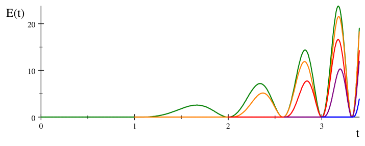
Figure 1: $E\left(t\right)$ for initial $x=1/2$, using potentials $V_{P}$, with $P=0$, $1$, $2$, $3$, & $4$.

The time for the zero-energy particle to traverse the complete unit interval in $x$ while moving through the $V_{P}$ potential (the $P$th “pseudo-half-cycle”) is always finite, for $P\neq 0$:

$$\Delta t_{P}=\left|\int_{0}^{1}\frac{dx}{v_{P}\left(x\right)}\right|=\frac{1}{\ln 2}~{}\left|\ln\left(1+\frac{1}{2\left(-\right)^{P}\left\lfloor\frac{1+P}{2}\right\rfloor}\right)\right|=\frac{1}{\ln 2}\ln\left(\frac{P+1}{P}\right)\ .$$ (45)

This transit time decreases monotonically as $P$ increases, with $\Delta t_{P}\underset{P\rightarrow\infty}{\sim}\frac{1}{P\ln 2}$.  Starting from an initial $x$, with initial $v>0$, the times at which changes in the potential occur, i.e. the times at which the particle encounters turning points, are obtained by summing these transit times and then adding $\Delta t_{0}\left(x\right)$.  The transit time sums are simple enough :

$$\sum_{N=1}^{P-1}\Delta t_{N}=\frac{\ln P}{\ln 2}\ .$$ (46)

Thus, a particle beginning at $x$, with initial $v>0$, will encounter its $P$th turning point, and the potential $V_{P}$ will switch on, at time $t_{P\text{ on}}\left(x\right)=\Delta t_{0}\left(x\right)+\frac{\ln P}{\ln 2}$.  The potential $V_{P}$ will remain in effect for a time span equal to the particle’s transit time, $\Delta t_{P}=t_{P+1\text{ on}}\left(x\right)-t_{P\text{ on}}\left(x\right)$, i.e. until the next potential $V_{P+1}$ switches on.

The potential index $P$ is in fact related to the action for the pseudo-half-cycle Morse .  For even $P$, we have $I\propto\int_{0}^{1}\cdots$, while for odd $P$, we have $I\propto\int_{1}^{0}\cdots$.  Thus (in the units chosen, the mass is $m=2$)

$$I_{P}=2\left(-1\right)^{P}\int_{0}^{1}v_{P}\left(x\right)dx=\left(4\left\lfloor\frac{1+P}{2}\right\rfloor+\left(-1\right)^{P}\right)I_{0}\ ,$$ (47)

where for the first pass through the complete unit interval the action is

$$I_{0}\equiv 2\int_{0}^{1}v\left(x\right)dx=\left(4\ln 2\right)\int_{0}^{1}\sqrt{x}\sqrt{1-x}\arcsin\sqrt{x}dx=\frac{1}{8}\left(\ln 2\right)\pi^{2}\ .$$ (48)

Moreover, $2\int_{0}^{1}\left(-v_{2k+1}\left(x\right)+v_{2k+2}\left(x\right)\right)dx=8\left(k+1\right)I_{0}$ for integer $k$, so after the initial crossing, the $\left(k+1\right)$st zigzag $1\rightarrow 0\rightarrow 1$ (“pseudo-full-cycle”) contributes to the action:

$$I_{k+1\ \leftrightarrows}=8\left(k+1\right)I_{0}\ .$$ (49)

The progressive deepening of the potential is also evident in the expanding phase-space trajectories for the evolving particle, where the switchbacks enhance the velocity after each encounter with a turning point ($v=0$).  For example, see Figure 2.

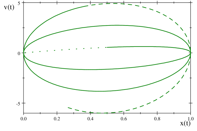
Figure 2: Phase-space trajectory $\left(x\left(t\right),v\left(t\right)\right)$ for $s=4$, with $x\left(0\right)=1/2$ and $v\left(0\right)=\frac{1}{4}\pi\ln 2$.  The solid portion of the curve is for $0\leq t\leq 3$, while the dashed extension is for $3\leq t\leq 3.5$.  The dotted portion of the curve is for negative times, $-\infty\leq t\leq 0$, with $x\left(-\infty\right)=v\left(-\infty\right)=0$.

This Figure provides a good opportunity to clarify the differences between conventional Hamiltonian and quasi-Hamiltonian systems.  The apparent failure to be a conventional Hamiltonian system is due entirely to the fact that a given phase-space trajectory seems to repeatedly cross itself at two points ($x\left(t\right)=0$, and $x\left(t\right)=1$, as shown in the Figure) and at various times. Thus a vector field on the phase space needed to describe the motion in the conventional Hamiltonian formalism would appear to be singular at those two points.

These phase-space singularities are tied to the branch point and Riemann surface sheet structure of the relevant analytic functions.  In fact, an alternate way to visualize the motion is as a trajectory on the sheets of a Riemann surface.  Consider the particle moving on the complex $x$ plane, and not just the real line segment $\left[0,1\right]$, the endpoints of which are now branchpoints.  There are cuts from $+1$ to $+\infty$ and from $0$ to $-\infty$.  The particle first moves along the real axis, approaches the cut at $+1$, and then goes around the branchpoint such that $\sqrt{x}\rightarrow\sqrt{x}$, $\sqrt{1-x}\rightarrow-\sqrt{1-x}$, and $\arcsin\rightarrow\pi-\arcsin$.  The particle returns along the real axis to the origin and encircles the branchpoint at $0$, such that $\sqrt{x}\rightarrow-\sqrt{x}$, $\sqrt{1-x}\rightarrow\sqrt{1-x}$, and $\arcsin\sqrt{x}\rightarrow-\arcsin\sqrt{x}$.  The particle then goes back to $+1$ and goes around it once more such that again $\sqrt{x}\rightarrow\sqrt{x}$, $\sqrt{1-x}\rightarrow-\sqrt{1-x}$, and $\arcsin\rightarrow\pi-\arcsin$.  The trajectory continues in this way, flipping signs and adding $\pi$s according to the formulae (43) and (44) Footnote2 .

For particles with initial $v>0$, a third way to picture the dynamics is in terms of the total distance traveled by the particle.  In this point of view, the successive $V_{P}$ patch together to form a continuous potential $V\left(X\right)$ on the real half-line, $X\geq 0$, as shown in Figure 3.  Indeed, the half-line may be thought of as a covering manifold of the unit interval in $x$, with the previous multi-valued functions of $x$ now single-valued functions of $X$.  To avoid stagnation at any of the cusps of $V\left(X\right)$, either physical or conceptual, in this picture the $E=0$ right-moving trajectories $X\left(t\right)$ may be considered as limits of positive energy right-movers, $X\left(t\right)=\lim_{E\downarrow 0}X_{E}\left(t\right)$.  This limiting process corresponds to the encirclement of the branch points in the Riemann surface picture.

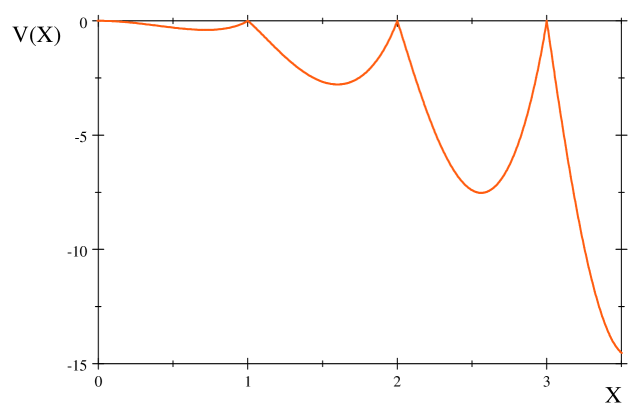
Figure 3: $V(X)$ where the total distance traveled by the particle is $X-x\left(t=0\right).$

Also, an “extended” phase space trajectory involving $X\left(t\right)$ and $dX\left(t\right)/dt$ gives some improvement over the situation depicted in Figure 2, with the trajectory no longer self-intersecting.  However, the corresponding phase-space vector field would still be singular with cusps appearing in $dX\left(t\right)/dt$ periodically in $X\left(t\right)$, similar to the cusps in the potential $V\left(X\right)$.  It is again possible to avoid the cusps by considering the extended phase space trajectories as limits of positive energy trajectories, but we leave that for the interested reader to pursue.

Finally, in terms of the coordinate transformation introduced in S , namely, the angle

$$\theta=\arcsin\sqrt{x}\ ,$$ (50)

the motion is completely unraveled, at least for $s=4$.  In that case $E=0$ implies $\left(\frac{d\theta\left(t\right)}{dt}\right)^{2}-\left(\ln 2\right)^{2}\theta^{2}\left(t\right)=0$, and the trajectory for all $t$ is just that of a particle moving in a repulsive quadratic potential (inverted SHO).  This is the easiest example solvable in closed-form by the Schröder method CZ .  The exponentially growing solution,  $\theta\left(t\right)=2^{t}\theta\left(0\right)$, whose values in the real-line cover of the circle are all physically distinct, immediately leads to $x\left(t\right)$ for the particle moving through the various $V_{P}\left(x\right)$, as is evident from (27).

To amplify our discussion of the physics encoded in the switchback potentials, we note that the chaotic behavior of the $s=4$ motion (i.e. the sensitive dependence on initial conditions) follows entirely from the behavior of the inverse Schröder function.  The sine function in (27) discards any integer multiple of $2\pi$.  So, for large and increasing times the trajectory $\left.x\left(t\right)\right|_{s=4}$ only depends on digits farther to the right of the decimal in the numerical value of the initial $\arcsin\sqrt{x}$, hence it is sensitive to those initial conditions.  Of course, this latter fact is well-known in the context of the discrete $s=4$ map, and has been discussed time and again in the literature for the case where $t$ is an integer (for example, see K ).  As is evident from (27) the discussion carries over mutatis mutandis to the continuous time case.  The only point we add here is to emphasize that it is $\Psi^{-1}$ which is responsible for the effect.  Insofar as $\Psi^{-1}$ follows from $\Psi$ and the latter follows directly from the potential (as well as the other way round, as discussed in our Introduction) the chaotic behavior follows directly from the specific multi-valued form of the potential.

For other values of $s$, from (7) and (6) we again have $x\left(t\right)=\Psi^{-1}\left(s^{t}\Psi\left(x,s\right),s\right)$, so the distinction between regular and chaotic behavior is again determined entirely by the asymptotic behavior of $\Psi^{-1}$, hence the asymptotic branch structure of $\Psi$, and hence the form of the switchback potentials.  The link between the analytic potential function and chaotic behavior is arguably somewhat subtle, inasmuch as it requires some computation to determine $\Psi$ and $\Psi^{-1}$, but the link is a direct one.  Having said that, there remains a case-by-case need for inspection of $\Psi^{-1}$ to determine chaos or its absence.  At this stage and in this paper, we do not purport to produce a universal analysis of all models — we only present methods that may facilitate such an analysis.

IV Conclusion

In summary, in this paper we

— Use a functional equation to convert nonlinear map equations into dynamical systems in the continuous time domain, thereby facilitating the study of such systems.

— Illustrate this holographic continuum interpolation technique with the well-known model of the logistic map, explicitly for the chaotic case $s=4$, an example which foreshadows an analysis for generic $s$.

— Construct an intricate sequence of switchback Hamiltonians which drive the system to just those phase-space trajectories resulting from such an analytic interpolation of the logistic map, and produce the familiar chaotic behavior for $s=4$.

For nontrivial systems such as the chaotic $s=4$ logistic map illustrated here, in order to produce the global features of the trajectories the potential of the underlying Hamiltonian system must change at each switchback of the motion, as occurs when turning points are reached in finite time.  Therefore we have called these systems quasi-Hamiltonian.  The trajectories dictate and completely determine the succession of switchback potentials, in a richly extended analogy of inverse scattering techniques.

For values of $s$ between $2$ and $4$, a numerical analysis pursuant to the techniques in this paper leads to quasi-Hamiltonian systems involving switchbacks among sequences of potentials, eventually producing trajectories that move between elaborate sets of turning points, in general.  This analysis is reported in full in a companion paper CV .  However, to make the present paper more self-contained, and perhaps more convincing as to the generality of the switchback effect, we have included some details for one other case ($s=3$) in an Appendix.

To conclude, we encourage experimenters to look in various settings for the particular type of continuous interpolates that we have described, including fluid dynamical experiments, ecological systems, and, more generally, any situation where an inherently continuous parameter (time, scale, etc.) has been routinely sampled only at predetermined discrete values.

V Appendix:  Some numerics for the $s=3$ case.

The coefficients in the series expansion of $\Psi$ may be computed recursively for any $s$, from (21).  While not immediately recognizeable as the series expansion of any well-known function, nonetheless, the coefficients may be used to estimate the radius of convergence of the series (20) by the simple ratio test:  $R_{\Psi}=\lim_{n\rightarrow\infty}R_{\Psi}\left(n\right)$, with $R_{\Psi}\left(n\right)\equiv\left|d\left(n-1\right)/d\left(n\right)\right|$.  To illustrate this consider the case $s=3$.  For this case numerical application of the ratio test leads to the data in Figure 4.

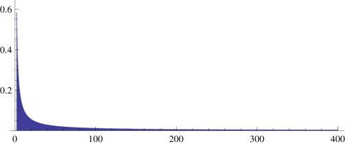
Figure 4: $R_{\Psi}\left(n\right)-s/4$ for $s=3$, plotted for $2\leq n\leq 400$, to show convergence towards $R_{\Psi}=3/4$.

From the numerical data we infer that $R_{\Psi}=3/4=\left.s/4\right|_{s=3}$, as indicated earlier in (22).  While this numerical demonstration is not a proof of convergence, of course, we believe it provides compelling evidence for convergence.

Other values of $s$ produce numerical data qualitatively the same as the $s=3$ case, with only one noteworthy difference:  While for $s>1$, the convergence of the numerical data to the expressions in (22) is from above, for $s<1$ the convergence is from below.

A similar numerical calculation for the coefficients in the expansion of the inverse function (18) suggests $\Psi^{-1}\left(x\right)$ is an entire function of $x$, for $s=3$, much like the closed-form results in (17).  That is to say, $R_{\Psi^{-1}}=\infty$ for $s=3.$

Combining the series data for $\Psi$, $\Psi^{-1}$, and $V$ with the functional equations obeyed by them leads to an accurate numerical determination of the functions and the switchback potentials, for any $s$.  The methods are described in detail in CV .  Numerical results for $\left.\Psi^{-1}\left(\frac{1}{2}~{}s^{t}\right)\right|_{s=3}$, with $-4\leq t\leq 9$, are shown in Figure 5 along with the expected asymptote, $\Psi_{\ast}^{-1}=2/3$.  This interval in $t$ corresponds to plotting $\Psi^{-1}\left(x\right)$ for $0\lesssim x\lesssim 10^{4}$.

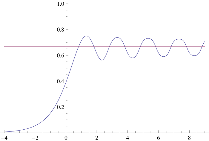
Figure 5: $\left.\Psi^{-1}\left(\frac{1}{2}~{}s^{t}\right)\right|_{s=3}$, in blue, for $-4\leq t\leq 9$, from series plus functional methods.

Numerical results for the first few potentials in the sequence, for $s=3$, are shown in Figure 6.

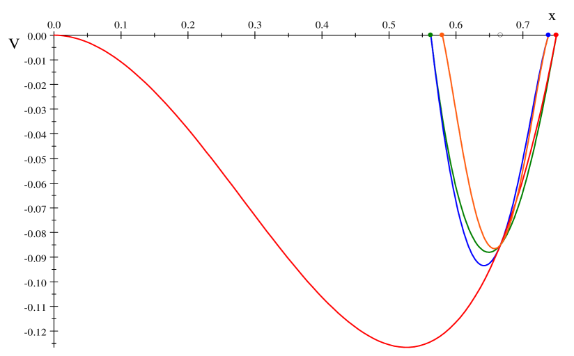
Figure 6: First four potentials in the sequence for $s=3$:  $V_{0}$ red, $V_{1}$ green, $V_{2}$ blue, and $V_{3}$ orange.

For this particular case, the sequence of potentials does not deepen progressively, but rather the sequence converges, albeit very slowly, onto the stable fixed point of the map, namely, $x_{\ast}=\left.1-\frac{1}{s}\right|_{s=3}=2/3$, shown in the Figure as a small circle on the $x$-axis.  Hence the zero-energy particle trajectory will also converge onto this fixed point, rigorously conserving $E=0$ in the process.

Although the particle trajectory is not chaotic for $s=3$, nevertheless the potentials are somewhat more exotic than the $s=4$ case in the sense that there are an infinite number of branch points for the $s=3$ case.  These may be obtained by iterating the action of the map on $x=1/2$.  That is to say, $\frac{1}{2}\rightarrow\frac{3}{4}=\allowbreak\frac{3}{2^{2}}\rightarrow\frac{9}{16}=\allowbreak\frac{3^{2}}{2^{4}}\rightarrow\frac{189}{256}=\allowbreak 3^{3}\frac{7}{2^{8}}\rightarrow\frac{37\,989}{65\,536}=\allowbreak 3^{4}7\frac{67}{2^{16}}\rightarrow\cdots$.  These branch points are shown as the turning points of the potential sequence, $\begin{array}[c]{ccccc}0.75,&0.562\,5,&0.738\,281\,,&0.579\,666\,,&\cdots\end{array}$, represented by colored dots on the $x$-axis in Figure 6.  The branch points may also be seen by flipping the graph of $\Psi^{-1}$ in Figure 5 about the SW-NE diagonal, in the usual way, to exhibit the various branches of $\Psi$.

This complicated branch structure for $s=3$ extends to other cases with $2<s<4$ and most likely accounts not only for the failure to render them in terms of simple, known functions, but also for some of the associated wide-spread mystique that surrounds $\Psi$ and $\Psi^{-1}$ in these cases.  Of course, $s=2$ and $s=4$ only have branch points at $x=1/2$, and at $x=0$ and $1$, respectively, as evident in the closed-form results (17) and as discussed in the text, so these cases are relatively bland by comparison.

References

-
(1)
T. Curtright and C. Zachos, J. Phys. A: Math. Theor.
42, 485208 (2009).
arXiv:0909.2424 [math-ph]. - (2) E. Schröder, Math. Ann. 3, 296-322 (1871).
-
(3)
L. Susskind, J. Math. Phys. 36, 6377 (1995).
arXiv:hep-th/9409089.
Also see http://en.wikipedia.org/wiki/Holographic_principle . - (4) The results (6) – (13) establish strong ties between the -functional method and the standard logical sequence conventionally used for time evolution, wherein one begins with a given potential and then computes the trajectory.
- (5) W. E. Ricker, Computation and interpretation of biological statistics of fish populations. Ottawa: Department of the Environment, Fisheries and Marine Service (1975).
- (6) R. M. May, Nature 261, 459-467 (1976).
- (7) P. Collet and J. P. Eckmann, Iterated Maps On The Interval As Dynamical Systems, Birkhäuser, Boston (1980).
- (8) M. J. Feigenbaum, Physica D 7, 16-39 (1983).
-
(9)
L. Kadanoff, Physics Today, 46-53 (December 1983).
Also see http://en.wikipedia.org/wiki/Logistic_map . - (10) P. Cvitanović, et al., Chaos: Classical and Quantum, http://chaosbook.org/ .
- (11) Perhaps this is not without precedent. Consider a small but macroscopic object made of weakly conducting dielectric material moving in the electric field produced by some charged surfaces. Occasionally the object might come in contact with one of the surfaces (i.e. hit a turning point) and exchange some significant amount of electric charge in the process. This would abruptly change the forces on the object, and correspondingly its potential, affecting the object’s motion and altering its subsequent trajectory. The potential could change abruptly again if the object were to come in contact with another charged surface. Of course, this process is more difficult to model than that of the logistic map.
- (12) The case gives a simple, closed-form result, namely, and . However, it is also pathological in the sense it does not yield a particle trajectory from (6) as written. Of course, a “scaling limit” might be considered, with fixed as . We leave this as an exercise for the reader.
- (13) http://www.physics.miami.edu/curtright/Schroeder.html
- (14) For odd , we may think of as a Morse index for the phase space pseudo-cycle: . Cf. Ch. 14 in M. C. Gutzwiller, Chaos in Classical and Quantum Mechanics, Springer, New York (1990).
- (15) By comparison to the electrically charged object described in a previous footnote, in the case of the particle interpolating the logistic map the charge acquired at the turning point is actually topological, as is clear in the Riemann surface point of view: The charge is just the winding number for the path of the particle around the branch points.
- (16) T. Curtright and A. Veitia, “Logistic Map Potentials” arXiv:1005.5030 [math-ph].