Anharmonic oscillation effect on the Davydov-Scott monomer in thermal bath

Abstract

The dynamics of Davydov-Scott monomer in a thermal bath with higher order amide-site’s displacement leads to anharmonic oscillation effect is investigated using full-quantum approach and the Lindblad formulation of master equation. The specific heat is calculated based on the thermodynamic partition function using the path integral method. The temperature dependence of the specific heat is studied. In the model the specific heat anomaly as pointed out in recent works by Ingold et.al. is also observed. However it is found that the anomaly occurs at high temperature region, and the anharmonic oscillation restores the positivity of specific heat.

I Introduction

The study of molecular biophysics began with Fr$\ddot{\mathrm{o}}$lich’s hypotheses which assumes that an excitation from an atomic vibration related to biological activity takeno . Based on this idea, Davydov has developed a quantum theory of protein to understand the mechanisms of energy transport in molecular protein, in particular alpha helix protein. The mechanism is an excitation energy of an amide-I is stabilized by its vibration in a combined excitation which propagate as a soliton scott ; scott2 . Most of studies in this field have been done at zero temperature, and little attention has been given at physiological temperatures.

The studies of Davydov soliton in physiological temperature is realized by the Davydov soliton interacting with thermal bath. While zero temperature calculation allows the existence of a soliton states in the proteins, there is an important question whether these states are stable at biological temperatures cruzeiro1 ; cruzeiro2 . Because the temperature effect may exchange heat energy with surrounding aqueous medium. The measurement of infrared absorption and Raman’s scattering of an crystallineacetanilide $(CH_{3}CONHC_{6}H_{5})_{x}$ at low temperature showed a new band closing to the amide-I band careri1 ; careri2 . The result is interpreted as a signature of Davydov’s soliton. The experiment using femtosecond IR spectroscopy realizing a band of the amide-I from acetanilide (ACN) and N-methylacetanide (NMA) shows the dependencies of absorption spectrum on temperature. At high temperature, the absorption spectrum shifts to higher frequency edler2 . Theoretical prediction using first order perturbation methods based on Davydov model gives soliton life time at the order of $O(10^{-12})$ s. This is very short time for biological processes in room temperature cottingham .

Using standard Davydov model, some numerical calculations showed that soliton is stable at 310K cruzeiro1 . The calculation based on trial function by Kapor et.al. showed that soliton is stable at 300K kapor1 . The result has also been confirmed in kapor2 .

From those results, it is important to study Davydov model involving the contact with thermal bath. The behavior of the system has attracted many interests in the last three decades. The interaction of a system with its environment is given by the dissipation effect in quantum system weiss ; rigo ; perceval . However, the dissipation effect leads to a serious problem for quantization procedure due to the broken Heisenberg’s relation. The most appropriate theory to resolve this problem is the Linblad formulation of master equation rigo ; perceval .

The first application of Linblad formulation of master equation to the protein model has been done by Cuevas et.al. cuevas . They used Davydov-Scott monomer model and showed that at 10K the quantum effect of amide-I vibration can not be neglected. Also at room temperature the semi classical approach might be a good approximation compared to the corresponding full quantum system. However the study was focused on the dynamical aspect of the system. Since the real world is affected by thermal fluctuation, it is important to study such system from statistical mechanics point of view.

In this paper the thermodynamic properties of Davydov-Scott monomer is investigated using Lindblad formulation and the partition function is calculated using path integral method feynmann . The path integral method is a powerful tool to investigate the properties of nonlinear dynamical systems with retarded interactions mazoli . In Sec. II the Hamiltonian of the system under consideration is described as a coupled harmonics oscillation i.e. the amide-I and amide-site oscillators. In addition to the original Davydov-Scott monomer, the higher order of amide-site displacement inducing the anharmonic oscillation effect of amide-site is also taken into account. This is motivated by the fact that the excitation and relaxation of collective modes of a protein are generally achieved via anharmonic interactions with other normal modes through energy exchange xie . In Sec. III the partition function is calculated using path integral approach to obtain the thermodynamic specific heat of the system which is then discussed in Sec. IV.

II Hamiltonian of Davydov-Scott monomer with anharmonic oscillation effect in Lindblad formulation of master equation

Considering the Davydov-Scott monomer, the excitation of the amide-I is described by the coordinate ($x$) and momentum ($p$) operators. On the other hand, the displacement and momentum operators of amide-site are expressed by $Q$ and $P$. The hamiltonian for Davydov-Scott monomer can then be written in the full quantum approach as follow,

$$H=\frac{p^{2}}{2m}+\frac{1}{2}m\mathbf{\omega}^{2}x^{2}-\frac{1}{4}\delta x^{4}+\frac{P^{2}}{2M}+V(Q)+\chi\frac{\partial V}{\partial Q}x\;,$$ (1)

where $\mathbf{\omega}$ is the intrinsic frequency of amide-I oscilation, $\chi$ measures the coupling between the amide-I excitation and the amide site vibration, $m$ ($M$) is the amide-I (amide-site) mass and $\delta$ is the anharmonic coefficient. Here the amide-site potential can generally be expanded around the origin,

$$V(Q) = V_{0}+\left.\frac{\partial V}{\partial Q}\right|_{Q=0}Q+\left.\frac{1}{2}\frac{\partial^{2}V}{\partial Q^{2}}\right|_{Q=0}Q^{2}$$ (2)

$$+\left.\frac{1}{6}\frac{\partial^{3}V}{\partial Q^{3}}\right|_{Q=0}Q^{3}+\left.\frac{1}{24}\frac{\partial^{4}V}{\partial Q^{4}}\right|_{Q=0}Q^{4}+\cdots\;.$$

The first term in Eq. (2) is a constant and can be scaled out. On the other hand, the equilibrium condition implies that the term of $Q$ vanishes due to $-\nabla V(Q)|_{Q=0}=0$. The third term is the harmonic oscillator one, while the remaining higher order terms represent the anharmonic contributions.

The original Davydov-Scott model assumes that the anharmonicity of amide-site is not important compared to the amide-I pouthier . The nonlinear effects appear only through exciton and amide-site coupling and higher order potential of excitons. However, recent experiment in biopolymer showed that the anharmonicity of polymer amide-site might be important go ; xie ; petr . The solid state experiments showed that at high temperature (room temperature), specific heat is not a constant anymore, but it is increasing. This fact can only be explained by taking into account the anharmonic oscillator term kittel .

In Eq. (2), the terms $Q^{3},Q^{5},\cdots$ represent the asymmetry of atom mutual repulsion, while the terms $Q^{4},Q^{6},\cdots$ represent the softening of vibration at large amplitudes kittel . Moreover, concerning the fact that the Davydov-Scott polymer has an identic monomer, it is plausible to assume that the asymmetry of atom mutual repulsion can be ignored. This yields,

$$V(Q)=\frac{1}{2}\,\kappa Q^{2}-\frac{1}{4}\lambda\,Q^{4}\;,$$ (3)

where $\kappa/2=1/2\,({\partial^{2}V}/{\partial Q^{2}})|_{Q=0}$ and $1/{24}\,({\partial^{4}V}/{\partial Q^{4}})|_{Q=0}=-\lambda/4$. Again, the second term induces the anharmonic oscillation effect in the system.

Unfortunately the term leads to a severe problem of describing the damping in open quantum systems, and it has been discussed for a long time. One of the known models dealing with this problem is the one dimensional damped harmonic oscillator (known as the Caldirola-Kanai Hamiltonian) um . In this model the momentum and coordinate operators are multiplied by $e^{-\gamma t}$ and $e^{\gamma t}$, where $\gamma$ is a damping factor.

In statistical mechanics, the behavior of an open system within system-plus-bath can be modeled by the density matrix formalism $\rho$. The equation of density matrix with hamiltonian $H$ and environment operator $R$ satisfy particular master equation weiss . It is usually restricted to weak system-bath interaction. The density operator gives the probability for the expected outcomes of measurements on the system. However, this formulation does not preserve density operator properties, that is hermiticity, unit trace, and positivity. The open quantum system theory which preserves density matrix properties can be realized using Lindblad formulation. In this theory, the interaction between Hamiltonian and thermal bath is realized by introducing some operators called Lindblad operators. The operators obey the master equation lindblad ,

$$\frac{\partial\rho}{\partial t}=-\frac{i}{\hbar}[H,\rho]+\frac{i}{2\hbar}\sum_{j}\left([L_{j},\rho L_{j}^{\dagger}]+[L_{j},\rho L_{j}^{\dagger}]\right)\;,\$$ (4)

where $L_{j}$ are the Lindblad operators. This choice is not unique and not necessarily Hermitian. Since $L$ must be the first order in $Q$ and $P$ perceval . The operators $H$ and $L$ denote the internal dynamics and environmental effects of the system. Throughout the paper, the Lindblad operators are put,

$$L_{1} = \sqrt{\gamma(1+\nu)}$$ (5)

$$\times\left(\sqrt{\frac{M\Omega}{2\hbar}}Q+i\sqrt{\frac{1}{2M\hbar\Omega}}P+\frac{\chi}{\hbar\Omega}x\right)\;,$$

$$L_{2} = \sqrt{\gamma\nu}\left(\sqrt{\frac{M\Omega}{2\hbar}}Q-i\sqrt{\frac{1}{2M\hbar\Omega}}P+\frac{\chi}{\hbar\Omega}x\right)\;,\$$ (6)

where $\gamma$ is a damping parameter related to the intensity of thermal bath, $\Omega=\sqrt{\kappa/M}$, $k_{B}$ is the Boltzmann constant, $T$ is temperature and $\nu=(e^{\hbar\Omega/k_{B}T}-1)^{-1}$ is the Bose-Einstein distribution.

Substituting Eqs. (5) and (6) into Lindblad master equation in Eq. (4),

$$\frac{\partial\rho}{\partial t} = -\frac{i}{\hbar}[H,\rho]-\frac{i\delta_{1}}{2\hbar}[Q,P\rho+\rho P]$$ (7)

$$-\frac{i\delta_{2}}{2\hbar}[x,P\rho+\rho P]-\frac{\delta_{3}}{2\hbar}\left[Q,[Q,\rho]\right]$$

$$-\frac{\delta_{4}}{2\hbar}\left[x,[Q,\rho]\right]-\frac{\delta_{5}}{2\hbar}\left[x,[x,\rho]\right]-\frac{\delta_{6}}{2\hbar}\left[P,[P,\rho]\right]\;,\$$

where $\delta_{i}$’s are the coefficient in the Lindblad operators,

$$\delta_{1} = \frac{\gamma}{2\hbar}(1+2\nu)\;,$$ (8)

$$\delta_{2} = \frac{\gamma\chi}{4\hbar\Omega}\sqrt{\frac{\omega}{\Omega}}(1+2\nu)\;,$$ (9)

$$\delta_{3} = \frac{\gamma M\Omega}{2\hbar}(1+2\nu)\;,$$ (10)

$$\delta_{4} = \frac{\gamma\chi}{2\hbar\Omega}\sqrt{Mm\Omega\omega}(1+2\nu)\;,$$ (11)

$$\delta_{5} = \frac{\gamma\chi^{2}m\omega}{4\hbar\Omega^{2}}(1+2\nu)\;,$$ (12)

$$\delta_{6} = \frac{\gamma}{2\hbar M\Omega}(1+2\nu)\;.$$ (13)

$\delta_{1,2}$ are the frictional damping rate, while $\delta_{3,4,5,6}$ are the quantum mechanical diffusion coefficients palchikov . This is the underlying model in the paper.

III Path integral calculation of partition function

In order to solve the master equation in Eq. (7), the resolution of a set of differential equations among the matrix elements of density operator with respect to a specific basis is required. This is usually provided by the eigen states of the system hamiltonian nakazato . But in the statistical mechanics it is not necessary to solve the master equation. Instead one can calculate the partition function ${\cal Z}$ using, for instance, path integral method.

III.1 Partition function

The density matrix can be obtained by performing a transformation $t\rightarrow\tau=-it=\beta\hbar$ with $\beta=1/(k_{B}T)$ feynmann . We assume that the quantum mechanical diffusion is dominant than the frictional damping rate such that it can be ignored. Then, the Lindblad master equation of the unnormalized $\rho$ can be rewritten as,

$$-\frac{\partial\rho}{\partial\beta}=H\rho+\triangle\rho\;,$$ (14)

where

$$\triangle\rho=\frac{i\delta_{3}}{2\hbar}Q^{2}\rho+\frac{i\delta_{4}}{2\hbar}xQ\rho+\frac{i\delta_{5}}{2\hbar}x^{2}\rho+\frac{i\delta_{6}}{2\hbar}P^{2}\rho\;.$$ (15)

It should be remarked here that, using this equation one can confirm the Linblad operators in Eqs. (5) and (6) lead to the right equilibrium. The proof is given in App. A.

The partition function corresponding to the master equation is given by feynmann ,

$${\cal Z}=\int{\cal D}[x(t)]e^{-\frac{1}{\hbar}S(x(t))}\;,$$ (16)

where $S(x(t))=\int_{0}^{\beta\hbar}(T+V)\mathrm{d}t^{\prime}$ is the Euclidean action corresponding to the equation.

Our interest is on the anharmonic amide-site interactions. Choosing the amide-site potential as Eq. (3) and taking into account only the first order of potential in the interaction, the action becomes feynmann ,

$${\cal S}_{xQ} = \int_{0}^{\tau}\mathrm{d}t\left(\frac{1}{2}m\dot{x}^{2}+\frac{1}{2}m\omega^{2}x^{2}-\frac{1}{2}\delta x^{4}+\chi xQ\right.$$ (17)

$$\left.+\frac{1}{2}M\dot{Q}^{2}+\frac{1}{2}\kappa Q^{2}-\frac{i\delta_{3}}{2}Q^{2}-\frac{1}{4}\lambda Q^{4}\right.$$

$$\left.-\frac{i\delta_{4}}{2}xQ-\frac{i\delta_{5}}{2}x^{2}-\frac{i\delta_{6}}{2}\dot{Q}^{2}\right)\;.$$

This yields,

$${\cal S}_{xQ} = \int_{0}^{\tau}\mathrm{d}t\left(\frac{1}{2}m\dot{x}^{2}+\frac{1}{2}\overline{k}x^{2}-\frac{1}{2}\delta x^{4}+\tilde{\chi}xQ\right.$$ (18)

$$\left.+\frac{1}{2}\overline{M}\dot{Q}^{2}+\frac{1}{2}\tilde{\kappa}Q^{2}-\frac{1}{4}\lambda Q^{4}\right)\;,$$

where $\tilde{\kappa}=\kappa-i\delta_{3}$ , $\overline{k}=k-i\delta_{5}$, $\overline{M}=M-i\delta_{6}$, $\tilde{\chi}=\chi-i/2\delta_{4}$ and $k=m\omega^{2}$. The amide-site is assumed to be more rigid than the amide-I. So the quantum fluctuation is dominated by the amide-I to enable us to use the Gaussian approximation. Making use of the Gaussian approximation, only the classical path of $Q$ contributes to the interaction term levit . Therefore the partition function becomes,

$${\cal Z}={\cal Z}_{x}{\cal Z}_{Q}\;,$$ (19)

where

$${\cal Z}_{x}=\int{\cal D}x\,\mathrm{e}^{-{\cal S}_{x}/\hbar}\;,$$ (20)

$${\cal Z}_{Q}=\int{\cal D}Q\,\mathrm{e}^{-{\cal S}_{Q}/\hbar}\;,$$ (21)

and the actions are,

$${\cal S}_{x} = \int_{0}^{\tau}\mathrm{d}t\left(\frac{1}{2}m\dot{x}^{2}+\frac{1}{2}\overline{k}x^{2}-\frac{1}{2}\delta x^{4}+\tilde{\chi}x\overline{Q}\right)\;,$$ (22)

$${\cal S}_{Q} = \int_{0}^{\tau}\mathrm{d}t\left(\frac{1}{2}\overline{M}\dot{Q}^{2}+\frac{1}{2}\tilde{\kappa}Q^{2}-\frac{1}{4}\lambda Q^{4}\right)\;.$$ (23)

III.2 Partition function for the amide-site

Further, one should solve the partition function of the amide-site (${\cal Z}_{Q}$). We use Gaussian approximation to solve the partition function. Under this approximation the general path can be expressed in the usual way as $Q=\overline{Q}+\breve{Q}$, where $\overline{Q}$ is the classical path and $\breve{Q}$ is the quantum path feynmann ; levit . Expanding the action in Taylor series ${\cal S}_{Q}$ becomes levit ,

$${\cal S}_{Q}={\cal S}_{Q}^{\mathrm{cl}}+\frac{1}{1!}\delta({\cal S}_{Q})^{\mathrm{cl}}+\frac{1}{2!}\delta^{2}({\cal S}_{Q})^{\mathrm{cl}}+\cdots\;.$$ (24)

Since the classical path satisfies the variational principles, $\delta{\cal S}_{Q}=0$, and taking only the second order,

$${\cal Z}_{Q}=\int{\cal D}Q\,\mathrm{exp}\left[\frac{1}{\hbar}\left({\cal S}_{Q}^{\mathrm{cl}}+\frac{1}{2!}\delta^{2}({\cal S}_{Q}^{\mathrm{cl}})\right)\right]\;.$$ (25)

This yields,

$${\cal Z}_{Q} = \mathrm{e}^{-{\cal S}_{Q}^{\mathrm{cl}}/\hbar}\int{\cal D}\breve{Q}\,\mathrm{exp}\left\{-\frac{1}{\hbar}\int\mathrm{d}t\frac{1}{2!}\left[\left(\frac{\partial^{2}{\cal L}^{\mathrm{cl}}_{\overline{Q}}}{\partial\overline{Q}^{2}}\right)\breve{Q}^{2}\right.\right.$$ (26)

$$\left.\left.+2\left(\frac{\partial^{2}{\cal L}^{\mathrm{cl}}_{\overline{Q}}}{\partial\overline{Q}\dot{\overline{Q}}}\right)\breve{Q}\dot{\breve{Q}}+\left(\frac{\partial^{2}{\cal L}^{\mathrm{cl}}_{\overline{Q}}}{\partial\dot{\overline{Q}}^{2}}\right)\dot{\breve{Q}}^{2}\right]\right\}\;,$$

where,

$${\cal L}^{\mathrm{cl}}_{\overline{Q}}=\frac{1}{2}\overline{M}\dot{\overline{Q}}^{2}+\frac{1}{2}\tilde{\kappa}\overline{Q}^{2}-\frac{1}{4}\lambda\overline{Q}^{4}\;.\$$ (27)

Calculating the second variation, and substituting the result into ${\cal Z}_{Q}$ in Eq. (26) one has,

$${\cal Z}_{Q} = \mathrm{e}^{-{\cal S}_{Q}^{\mathrm{cl}}/\hbar}\,{\cal Z}_{Q_{0}}$$ (28)

$$= \mathrm{exp}\left[-\frac{1}{\hbar}\int_{0}^{\tau}\mathrm{d}t\left(\frac{1}{2}\overline{M}\dot{\overline{Q}}^{2}+\frac{1}{2}\tilde{\kappa}\overline{Q}^{2}-\frac{1}{4}\lambda\overline{Q}^{4}\right)\right]$$

$$\times\int{\cal D}\breve{Q}\,\mathrm{exp}\left[-\frac{1}{\hbar}\int_{0}^{\tau}\mathrm{d}t\right.$$

$$\left.\times\left(\frac{1}{2}\overline{M}\dot{\breve{Q}}^{2}+\frac{1}{2}\tilde{\kappa}\breve{Q}^{2}-\frac{3}{2}\lambda\overline{Q}^{2}\breve{Q}^{2}\right)\right]\;.$$

The equation of motion for $\overline{Q}$ in Euclidean coordinate is given by,

$$\frac{d^{2}\overline{Q}}{dt^{2}}-\overline{\Omega}^{2}\overline{Q}+\frac{\lambda}{\overline{M}}\overline{Q}^{3}=0\;,$$ (29)

where $\overline{\Omega}^{2}={\tilde{\kappa}}/\overline{M}$. In this paper the solution is taken to have the form of,

$$\overline{Q}=\overline{Q}_{0}\,\mathrm{sech}(\overline{\Omega}t)\;,$$ (30)

which leads to $\overline{Q}_{0}=\overline{\Omega}\sqrt{{(2M)}/\lambda}$. This choice is motivated by the fact that the Davydov model is the self-trapping of its energy, i.e. it should be localized. Substituting this solution into classical action and using the identity $1-\mathrm{sech}^{2}x=\tanh^{2}x$, one obtains,

$${\cal S}_{Q}^{\mathrm{cl}}=A_{1}\tanh\left(\overline{\Omega}\hbar\beta\right)+A_{2}\tanh^{3}\left(\overline{\Omega}\hbar\beta\right)\;,$$ (31)

where,

$$A_{1} = \frac{1}{2}\overline{M}\overline{\Omega}\overline{Q}_{0}^{2}-\frac{1}{4}\frac{\lambda}{\overline{\Omega}}\overline{Q}_{0}^{4}\;,$$ (32)

$$A_{2} = \frac{1}{12}\frac{\lambda}{\overline{\Omega}}\overline{Q}_{0}^{4}-\frac{1}{2}\overline{M}\overline{\Omega}\overline{Q}_{0}^{2}\;.$$ (33)

Now the problem is turned into solving the prefactor in the path integral,

$${\cal Z}_{Q_{0}} = \int{\cal D}\breve{Q}\,\mathrm{exp}\left[-\frac{1}{\hbar}\int_{0}^{\tau}\mathrm{d}t\left(\frac{1}{2}\overline{M}\dot{\breve{Q}}^{2}\right.\right.$$ (34)

$$\left.\left.+\frac{1}{2}\kappa\breve{Q}^{2}-\frac{3}{2}\lambda\overline{Q}^{2}\breve{Q}^{2}\right)\right]\;.$$

Using semi-classical approximation it can be rewritten as ranfagui ,

$$\mathcal{Z}_{Q_{0}}=\frac{1}{\sqrt{2\pi\hbar}}\left.\left(\frac{\delta^{2}{\cal S}_{\breve{Q}_{0}}}{\delta\breve{Q}^{2}}\right)^{1/2}\right|_{\overline{Q}}\;,$$ (35)

and its second order variation is given by,

$$\left.\frac{\delta^{2}{\cal S}_{\breve{Q}_{0}}}{\delta\breve{Q}^{2}}\right|_{\overline{Q}} = \frac{\tau\sqrt{\overline{M}\tilde{\kappa}}}{2\pi\hbar}\int^{\tau}_{0}\mathrm{d}t\left(\frac{\partial^{2}{\cal L}^{\mathrm{cl}}_{\overline{Q}}}{\partial\dot{\overline{Q}}^{2}}\ddot{\overline{Q}}^{2}\right.$$ (36)

$$\left.+2\frac{\partial^{2}{\cal L}^{\mathrm{cl}}_{\overline{Q}}}{\partial\dot{\overline{Q}}\partial\overline{Q}}\overline{Q}\dot{\overline{Q}}+\frac{\partial^{2}{\cal L}^{\mathrm{cl}}_{\overline{Q}}}{\partial\overline{Q}^{2}}\dot{\overline{Q}}^{2}\right)\;.$$

The result is,

$$\left.\frac{\delta^{2}{\cal S}_{\breve{Q}_{0}}}{\delta\breve{Q}^{2}}\right|_{\overline{Q}}=\frac{\tau\sqrt{\overline{M}\tilde{\kappa}}}{2\pi\hbar}\int^{\tau}_{0}\mathrm{d}t\left[\overline{M}\ddot{\overline{Q}}^{2}+\left(-\tilde{\kappa}+3\lambda\overline{Q}^{2}\right)\dot{\overline{Q}}^{2}\right]\;,$$ (37)

and by substituting $\overline{Q}$ in Eq. (30),

$$\left.\frac{\delta^{2}{\cal S}_{\breve{Q}_{0}}}{\delta\breve{Q}^{2}}\right|_{\overline{Q}} = \frac{\beta\sqrt{\overline{M}\tilde{\kappa}}}{2\pi}\left[\Lambda_{1}\,\mathrm{sech}^{4}(\overline{\Omega}\hbar\beta)\tanh(\overline{\Omega}\hbar\beta)\right.$$ (38)

$$\left.\times\left(\cosh(2\overline{\Omega}\hbar\beta)-3\right)+\Lambda_{2}\tanh^{3}(\overline{\Omega}\hbar\beta)\right.$$

$$\left.+\Lambda_{3}\mathrm{sech}^{2}(\overline{\Omega}\hbar\beta)\tanh^{3}(\overline{\Omega}\hbar\beta)\right.$$

$$\left.\times(4+\cosh(2\overline{\Omega}\hbar\beta)\right]\;,$$

where,

$$\Lambda_{1} = \frac{1}{2}\overline{M}\overline{Q}_{0}^{2}\;,$$ (39)

$$\Lambda_{2} = -\frac{1}{3}\tilde{\kappa}\overline{\Omega}\overline{Q}_{0}^{2}\;,$$ (40)

$$\Lambda_{3} = \frac{1}{5}\lambda\overline{\Omega}\overline{Q}_{0}^{4}\;.$$ (41)

Finally, the complete partition function for the amide-site is obtained,

$${\cal Z}_{Q} = \frac{1}{2\pi}\sqrt{\frac{\beta}{\hbar}}(\overline{M}\tilde{\kappa})^{1/4}\left\{\Lambda_{1}\,\mathrm{sech}^{4}(\overline{\Omega}\hbar\beta)\tanh(\overline{\Omega}\hbar\beta)\right.$$ (42)

$$\left.\times(\cosh(2\overline{\Omega}\hbar\beta)-3)-\Lambda_{2}\tanh^{3}(\overline{\Omega}\hbar\beta)\right.$$

$$\left.+\Lambda_{3}\,\mathrm{sech}^{2}(\overline{\Omega}\hbar\beta)\tanh^{3}(\overline{\Omega}\hbar\beta)(4+\cosh(2\overline{\Omega}\hbar\beta))\right\}^{1/2}$$

$$\times\mathrm{exp}\left[-\frac{1}{\hbar}(A_{1}\tanh(\overline{\Omega}\hbar\beta)+A_{2}\tanh^{3}(\overline{\Omega}\hbar\beta))\right]\;.$$

III.3 Partition function for the amide-I

For the action of amide-I, ${\cal S}_{x}$, the partition function is,

$${\cal Z}_{x} = \int{\cal D}x\,\mathrm{exp}\left[-\frac{1}{\hbar}\int\mathrm{d}t\left(\frac{1}{2}m\dot{x}^{2}+\frac{1}{2}\overline{k}x^{2}+\tilde{\chi}x\overline{Q}\right.\right.$$ (43)

$$\left.\left.-\frac{1}{2}\delta x^{4}\right)\right]\;.$$

Dividing $x$ into classical path $\overline{x}$ and quantum path $\breve{x}$, i.e. $x=\overline{x}+\breve{x}$, and again using the Gaussian approximation, the classical path is,

$${\cal S}_{x}^{\mathrm{cl}}=\int\mathrm{d}t\left(\frac{1}{2}m\dot{\overline{x}}^{2}+\frac{1}{2}\overline{k}\overline{x}^{2}-\frac{1}{2}\delta\overline{x}^{4}+\tilde{\chi}\overline{x}\overline{Q}\right)\;.$$ (44)

This can be solved by determining the classical path which is the solution of following equation,

$$m\ddot{\overline{x}}-\overline{k}\overline{x}+2\delta\overline{x}^{3}=\tilde{\chi}\overline{Q}_{0}\,\mathrm{sech}(\overline{\Omega}t)\;.$$ (45)

However this is hard to be solved analytically. Instead one can use the perturbation method, i.e. calculating the solutions order by order $\overline{x}=\overline{x}^{0}+\varepsilon\overline{x}^{1}+\cdots$. Note that the inhomogeneous term is assumed being generated from the leading order. Substituting this expansion into Eq. (45) up to the leading orders one has,

$$m\ddot{\overline{x}}^{0}-\overline{k}\overline{x}^{0}+2\delta\overline{x}^{03}=0\;,$$ (46)

for the lowest order and,

$$m\ddot{\overline{x}}^{1}-\overline{k}\overline{x}^{1}+6\delta\overline{x}^{02}\overline{x}^{1}=\tilde{\chi}\overline{Q}_{0}\,\mathrm{sech}(\overline{\Omega}t)\;,\$$ (47)

for the first order. Similar to the solution in the amide-site coordinate, since $\delta<\overline{k}$, the solution for the zeroth order is,

$$\overline{x}^{0}=\overline{X}_{0}\,\mathrm{sech}(\overline{\omega}t)\;,$$ (48)

where $\overline{\omega}=\overline{k}/m$, $\overline{X}_{0}=\overline{\omega}\sqrt{m/{\delta}}$ after transforming $t\rightarrow it$. In this solution $\delta$ must not be zero. For the first order, the solution is $x^{1}=x^{1}_{h}+x^{1}_{p}$ and $x^{1}_{h}$ satisfies,

$$\ddot{\overline{x}}_{h}^{1}-\overline{\omega}^{2}\overline{x}_{h}^{1}+6\frac{\delta}{m}\overline{X}_{0}^{2}\,\mathrm{sech}^{2}(\overline{\omega}t)\overline{x}_{h}^{1}=0\;.$$ (49)

Performing a transformation $\tau=\tanh(\overline{\omega}t)$ one gets the associated Legendre equation,

$$\frac{\mathrm{d}}{\mathrm{d}\tau}\left[(1-\tau^{2})\frac{\mathrm{d}\overline{x}_{h}^{1}}{\mathrm{d}\tau}\right]+\left[l(l+1)+\frac{n^{2}}{1-\tau^{2}}\right]\overline{x}_{h}^{1}=0\;,$$ (50)

where $n^{2}=\overline{\omega}$ and $l(l+1)=6{\delta}/{(m\overline{\omega})}\overline{X}_{0}^{2}$. The solution is $x_{h}^{1}=x_{h_{0}}^{1}P_{l}^{n}(\tanh(\overline{\omega}t))$ where $P_{l}^{n}(\tau)$ is the associated Legendre function. Particularly its solution satisfies,

$$m\ddot{\overline{x}}_{p}^{1}-m\overline{\omega}^{2}\overline{x}_{p}^{1}+6\delta\overline{X}_{0}^{2}sech^{2}(\overline{\omega}t)\overline{x}_{p}^{1}=\tilde{\chi}\overline{Q}_{0}\,\mathrm{sech}(\overline{\Omega}t)\;.$$ (51)

The solution of this equation can be written using Green function $G(\tau,\tau^{\prime})$ as follow,

$$\overline{x}_{p}^{1}=\frac{\tilde{\chi}\overline{Q}_{0}}{m}\int\mathrm{d}\tau^{\prime}\,G(\tau,\tau^{\prime})\mathrm{sech}\left[\frac{\overline{\Omega}}{\overline{\omega}}\tanh^{-1}(\tau^{\prime})\right]\;,\$$ (52)

and the Green function is governed by,

$$\frac{\mathrm{d}}{\mathrm{d}\tau}\left[(1-\tau^{2})\frac{\mathrm{d}G(\tau,\tau^{\prime})}{\mathrm{d}\tau}\right]+\left[l(l+1)-\frac{m^{2}}{1-\tau^{2}}\right]G(\tau,\tau^{\prime})$$

$$=-\delta(\tau-\tau^{\prime})\;.$$ (53)

The Green function is given by filho , $G(\tau,\tau^{\prime})=(-1)^{n}P_{l}^{n}(\tau_{<})Q_{l}^{n}(\tau_{>})$ with $Q_{l}^{n}(\tau)$ is the associated Legendre functions of the second kind. Its complete solution is,

$$\overline{x} = \overline{X}_{0}\,\mathrm{sech}(\overline{\omega}t)+\varepsilon\left[x_{h_{0}}^{1}P_{l}^{n}(\tanh(\overline{\omega}t))\right.$$ (54)

$$\left.+\frac{\tilde{\chi}\overline{Q}_{0}}{m}\int\mathrm{d}\tau^{\prime}\,G(\tau,\tau^{\prime})\mathrm{sech}\left(\frac{\overline{\Omega}}{\overline{\omega}}\tanh^{-1}(\tau^{\prime})\right)\right]\;.\$$

Substituting this result into Eq. (44) one obtains the classical action. On the other hand, the classical action up to the first order is given by,

$${\cal S}_{x}^{\mathrm{cl}} = \Delta_{1}\tanh(\overline{\omega}\hbar\beta)+\Delta_{2}\tanh^{3}(\overline{\omega}\hbar\beta)$$

$$+\Delta_{3}\int_{0}^{\beta\hbar}\mathrm{d}t\,\mathrm{sech}(\overline{\omega}t)\,\mathrm{sech}(\overline{\Omega}t)$$

$$+\varepsilon(F_{1}+F_{2}+F_{3}+F_{4}+F_{5}+F_{6}+F_{7}+F_{8})\;,\$$

where,

$$\Delta_{1} = \frac{1}{2}m\overline{\omega}\overline{X}_{0}^{2}+\frac{\delta}{3\overline{\omega}}\overline{X}_{0}^{4}\;,$$ (56)

$$\Delta_{2} = -\frac{m}{2}\overline{\omega}\overline{X}_{0}^{2}+\frac{\delta\overline{X}_{0}^{4}}{6\overline{\omega}}\;,$$ (57)

$$\Delta_{3} = -\frac{1}{2}\tilde{\chi}\overline{X}_{0}\overline{Q}_{0}\;,$$ (58)

and $F_{i}$’s are given in App. B.

Performing the same procedure as done in the previous subsection, one should consider the prefactor of $\mathcal{Z}_{x}$, that is,

$$\mathcal{Z}_{x^{0}}=\frac{1}{\sqrt{2\pi\hbar}}\left.\left(\frac{\delta^{2}{\cal S}_{\breve{x}^{0}}}{\delta\breve{x}^{2}}\right)^{1/2}\right|_{\overline{x}}\;,\$$ (59)

where the second order variation is given by,

$$\left.\frac{\delta^{2}{\cal S}_{\breve{x}^{0}}}{\delta\breve{x}^{2}}\right|_{\overline{x}} = \frac{\beta\sqrt{m\overline{\omega}^{2}}}{2\pi}\int^{\tau}_{0}\mathrm{d}t\left(\frac{\partial^{2}{\cal L}^{\mathrm{cl}}_{\overline{x}}}{\partial\dot{\overline{x}}^{2}}\ddot{\overline{x}}^{2}\right.$$ (60)

$$\left.+2\frac{\partial^{2}{\cal L}^{\mathrm{cl}}_{\overline{x}}}{\partial\dot{\overline{x}}\partial\overline{x}}\overline{x}\dot{\overline{x}}+\frac{\partial^{2}{\cal L}^{\mathrm{cl}}_{\overline{x}}}{\partial\overline{x}^{2}}\dot{\overline{x}}^{2}\right)\;,$$

and,

$${\cal L}^{\mathrm{cl}}_{\overline{x}}=\frac{1}{2}m\dot{\overline{x}}^{2}-\frac{1}{2}m\overline{\omega}^{2}\overline{x}^{2}+\frac{1}{2}\delta\overline{x}^{4}+\tilde{\chi}\overline{x}\overline{Q}\;,$$ (61)

which yields,

$$\left.\frac{\delta^{2}{\cal S}_{\breve{x}^{0}}}{\delta\breve{x}^{2}}\right|_{\overline{x}} = \frac{\beta\sqrt{m\overline{\omega}^{2}}}{2\pi}\int^{\beta\hbar}_{0}\mathrm{d}t\,$$ (62)

$$\times\left[m\ddot{\overline{x}}^{2}-(m\overline{\omega}^{2}+3\delta\overline{x}^{2})\dot{\overline{x}}^{2}\right]\;.\$$

Substituting Eq. (54) into Eq. (62) and keeping only the first order,

$$\left.\frac{\delta^{2}{\cal S}_{\breve{x}^{0}}}{\delta\breve{x}^{2}}\right|_{\overline{x}}=\frac{\beta\sqrt{m\overline{\omega}^{2}}}{2\pi}\times$$

$$\left[\Gamma_{1}\,\mathrm{sech}^{4}(\overline{\omega}\hbar\beta)\tanh(\overline{\omega}\hbar\beta)(\cosh(2\overline{\omega}\hbar\beta)-3)\right.$$

$$\left.+\Gamma_{2}\tanh^{3}(\overline{\omega}\hbar\beta)\right.$$

$$\left.+\Gamma_{3}(4+\cosh(2\overline{\omega}\hbar\beta))\mathrm{sech}^{2}(\overline{\omega}\hbar\beta)\tanh^{3}(\overline{\omega}\hbar\beta)\right.$$

$$\left.+\varepsilon(G_{1}+G_{2}+G_{3}+G_{4}+G_{5}\right.$$

$$\left.+G_{6}+G_{7}+G_{8}+G_{9}+G_{10})\right]\;,\ \;.\$$ (63)

where,

$$\Gamma_{1} = -\frac{m}{2}\overline{\omega}^{3}\overline{X}_{0}^{2}\;,$$ (64)

$$\Gamma_{2} = \frac{m\overline{\omega}^{3}\overline{X}_{0}^{2}}{3}\;,$$ (65)

$$\Gamma_{3} = \frac{\delta\overline{\omega}\overline{X}_{0}^{4}}{5}\;,$$ (66)

and $G_{i}$’s are given in the App. C..

Hence, the partition function ${\cal Z}_{x}$ is obtained,

$${\cal Z}_{x}=\left(\frac{\beta\sqrt{m\overline{\omega}^{2}}}{4\pi^{2}\hbar}\right)^{1/2}\times$$

$$\left[-\Gamma_{1}\,\mathrm{sech}^{4}(\overline{\omega}\hbar\beta)\tanh(\overline{\omega}\hbar\beta)(\cosh(2\overline{\omega}\hbar\beta)-3)\right.$$

$$\left.+\Gamma_{2}\tanh^{3}(\overline{\omega}\hbar\beta)\right.$$

$$\left.+\Gamma_{3}(4+\cosh(2\overline{\omega}\hbar\beta))\,\mathrm{sech}^{2}(\overline{\omega}\hbar\beta)\tanh^{3}(\overline{\omega}\hbar\beta)\right.$$

$$\left.+\varepsilon(G_{1}+G_{2}+G_{3}+G_{4}+G_{5}\right.$$

$$\left.+G_{6}+G_{7}+G_{8}+G_{9}+G_{10})\right]^{1/2}$$

$$\times\mathrm{exp}\left\{-\frac{1}{\hbar}\left[\Delta_{1}\tanh(\overline{\omega}\hbar\beta)+\Delta_{2}\tanh^{3}(\overline{\omega}\hbar\beta)\right.\right.$$

$$\left.\left.+\Delta_{3}\int_{0}^{\beta\hbar}\mathrm{d}t\,\mathrm{sech}(\overline{\omega}t)\,\mathrm{sech}(\overline{\Omega}t)\right.\right.$$

$$\left.\left.+\varepsilon(F_{1}+F_{2}+F_{3}+F_{4}+F_{5}+F_{6}+F_{7}+F_{8})\right]\right\}\;.\$$ (67)

Finally, the complete partition function density of Davydov-Scott monomer in thermal bath, ${\cal Z}={\cal Z}_{x}\,{\cal Z}_{Q}$, is obtained from Eqs. (42) and (67).

IV Thermodynamical properties of Davydov-Scott monomer

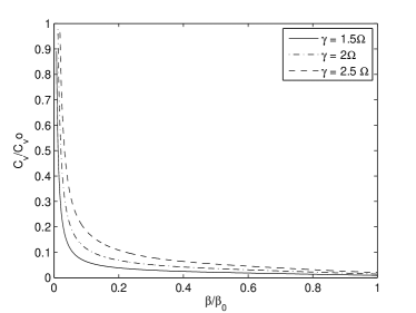
Figure 1: The temperature dependence of normalized specific heat for various values of $\gamma$ with $\lambda=1$.

From physical point of view, the Davydov-Scott monomer is a harmonic oscillator coupled to a quantum excitation. Using Euler-Lagrange equation, one can derive the appropriate equation of motion (EOM) from the action in Eq. (17). Although solving of the EOM is very interesting and attractive, but it has a little physical significant due to unobservable individual molecular motion of the Davydov-Scott monomer. Therefore in this paper let us consider thermodynamic observable as specific heat feynmann ,

$$C=k_{B}\beta^{2}\frac{\partial^{2}\ln({\cal Z})}{\partial\beta^{2}}\;.\$$ (68)

Some previous works considering similar model as the Hamiltonian in Eq. (1) to study the Davydov-Scott monomer in thermal bath, for example the semiclassical approach in cuevas . It has been argued that using Lindblad formulation the semiclassical limit is a good approximation to the corresponding full quantum treatment at biological temperatures in the highly underdamped and harmonic limits. In the semiclassical approximation, the coupling between Davydov-Scott monomer with thermal bath is described by Langevin equation of the amide-site displacement characterized by $\gamma$ and $\Omega$ cruzeiro2 . If the stochastic force represents the thermal bath is zero, the equation is reduced into the damped harmonic oscillator. There are three regions regarding the values of $\gamma$ and $\Omega$, that is $\gamma<2\Omega$ for the underdamped condition, $\gamma=2\Omega$ for the critical damped condition and $\gamma>2\Omega$ for the overdamped condition. In the Lindblad formulation the damping coefficient $\gamma$ represents the relaxation time due to interaction with the environment. The higher values of $\gamma$ corresponds to the shorter relaxation time. The previous work by Cuevas et.al. has established that the semiclassical approximation is equivalent to the full quantum approach (for biological temperature) as long as $\gamma\ll 2\Omega$. Otherwise, the oscilation frequency of the observable would be different cuevas .

In this paper, the analysis is done for the above three criterions. The values of parameters used throughout numerical calculation are $M=6.3\times 10^{-26}$ kg, $m=7.3\times 10^{-26}$ kg, $\kappa=10$ Nm^-1 and $\omega=1660$ cm^-1 cuevas ; sinkala , while $\lambda=9$. The behavior of specific heat in term of temperature is shown in Fig. 1 for various damping parameter $\gamma$, Figs. 2$-$4 for various strength of anharmonic oscillation in three damping conditions and Fig. 5 for various $\gamma$ in the underdamped case. The results are similar with the previous ones obtained in the calculation of a system with anharmonic amide-site zoli .

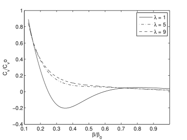
Figure 2: The temperature dependence of normalized specific heat for various values of $\lambda$ for the underdamped condition with $\gamma=0.1\Omega$.

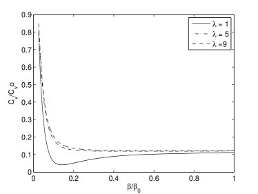
Figure 3: The temperature dependence of normalized specific heat for various values of $\lambda$ for the critical damped condition with $\gamma=2\Omega$.

In the present case the damping coefficients are represented by the coefficients $\delta_{1}\sim\delta_{6}$. In particular, $\delta_{1}$ appears in the kinetic terms, and can then be interpreted as the ’effective mass’ of amide-site vibration. Further, $\delta_{3}$ appears in the harmonic potential as the ’effective elastic constant’. Hence it can be argued that the environment effects to the amide-site vibration occur through the kinetic term and the harmonic potential. The coefficient $\delta_{4}$ represents the strength of the interaction between amide-I.and the system.

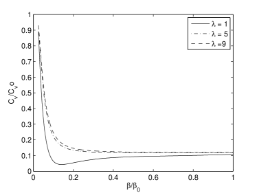
Figure 4: The temperature dependence of normalized specific heat for various values of $\lambda$ for the overdamped condition with $\gamma=2.5\Omega$.

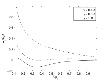
Figure 5: The temperature dependence of normalized specific heat for the underdamped condition with various values of $\gamma<2\Omega$ and $\lambda=1$.

From the figures, the specific heat asymptotically approaches to zero at low temperature and to infinity at high temperature. Actually $\phi^{4}$ potential oscillator interacting with electron and also the anharmonic oscillator give similar profiles schwarcz . Large environment effect causes the Davydov-Scott monomer to increase the energy and then the temperature to achieve the equilibrium state. Correspondingly the vibration frequency is also affected by the damping coefficients since $\omega=\sqrt{\tilde{\kappa}/\overline{M}}=\sqrt{{(\kappa+i\delta_{3})}/{(M+i\delta_{2})}}$. These results indicate that the interaction between Davydov-Scott monomer and thermal bath depend on the strength of the coupling of system and environment. Recent study of the open quantum system also shows that the canonical equilibrium state of an open quantum system depends explicitly on the system-bath coupling strength ingold ; campisi .

In particular, from Fig. 2 the anomaly of specific heat that becomes negative for certain parameter sets at high temperature region is observed. The same phenomena have been pointed out by Ingold et.al. ingold ; ingold2 . In the current case, the anomaly especially appears for the underdamped condition as shown in Figs. 2 and 5. It is also found that the negative specific heat is restored at large $\lambda$ and $\gamma$, i.e. for large anharmonic oscillation and intensity of thermal bath.

It should also be remarked that one cannot take $\lambda=0$ (no oscilation effect) since all results are obtained from Eq. (30) which is a special case with $\lambda\neq 0$ condition.

V Summary

The interaction of Davydov-Scott monomer with thermal bath is investigated using the Lindblad formulation of master equation. In contrast with previous work by Cuevas et.al. cuevas , the anharmonic oscillation term of amide-site is taken into account. Adopting similar Lindblad operators used in cuevas , the master equation of the system is obtained. Instead of solving the equation of motion, the thermodynamic partition function and in particular specific heat are calculated using the path integral methods.

It is shown that the coupling with the environment contributes to the kinetic term, the harmonic potential of amide-site vibration and the anharmonic term of amide-I.

The anomaly of specific heat that becomes negative for certain parameter sets at high temperature region is observed as pointed out by Ingold et.al. in the case of pure open quantum systems ingold ; ingold2 . However, it is found that the negative specific heat is restored for large anharmonic oscillation effect. In contrast to these results, Ingold et.al. have found that the anomaly occurs at low temperature region. This discrepancy can be explained as the consequences of different approaches adopted to model the interaction between the system and the thermal bath. Ingold et.al. has represented the interaction in a set of harmonic oscillators which becomes the coupled harmonic oscillator at classical approximation. In contrary, in the present approach the thermal bath is represented in a set of Lindblad operators which becomes the underdamped harmonic oscillator at classical approximation.

From the figures, it can in general be concluded that the anharmonic oscillation contributes constructively to the specific heat.

Appendix A The equilibrium state with the Lindblad operators in Eqs. (5) and (6)

Let us investigate the equilibrium state in the present case. Substituting the amide-site potential in Eq. (3) and the leading interaction term in Eq. (3) into the Lindblad master equation in Eq. (14) yields,

$$-\frac{\partial\rho}{\partial\beta} = \frac{1}{2m}\frac{\partial^{2}\rho}{\partial x^{2}}+\frac{1}{2}m\omega^{2}x^{2}\rho+\frac{i\delta_{5}}{2\hbar}x^{2}\rho-\frac{1}{4}\delta x^{4}\rho$$ (69)

$$+\frac{1}{2M}\frac{\partial^{2}\rho}{\partial Q^{2}}+\frac{i\delta_{6}}{2\hbar}\frac{\partial^{2}\rho}{\partial Q^{2}}+\frac{1}{2}\kappa Q^{2}\rho+\frac{i\delta_{3}}{2\hbar}Q^{2}\rho$$

$$+\frac{1}{4}\lambda Q^{4}\rho+\chi xQ\rho+\frac{i\delta_{4}}{2\hbar}xQ\rho\,.$$

This can be rearranged to be,

$$-\frac{\partial\rho}{\partial\beta} = \frac{1}{2m}\frac{\partial^{2}\rho}{\partial x^{2}}+\left[\frac{1}{2}m\omega^{2}+\frac{i\delta_{5}}{2\hbar}\right]x^{2}\rho-\frac{1}{4}\delta x^{4}\rho$$ (70)

$$+\left[\frac{1}{2M}+\frac{i\delta_{6}}{2\hbar}\right]\frac{\partial^{2}\rho}{\partial Q^{2}}+\left[\frac{1}{2}\kappa+\frac{i\delta_{3}}{2\hbar}\right]Q^{2}\rho$$

$$+\frac{1}{4}\lambda Q^{4}\rho+\left[\chi+\frac{i\delta_{4}}{2\hbar}\right]xQ\rho\,.$$

On the other hand, the average value of any operator $A$ at a thermal equilibrium is given by feynmann ,

$$\langle\langle A\rangle\rangle=\frac{\mathrm{Tr}(\mathrm{e}^{-\beta H}A)}{\mathrm{Tr}(\mathrm{e}^{-\beta H})}\,,$$ (71)

or in the integral form,

$$\langle\langle A\rangle\rangle=\frac{\int\rho(x)A(x)\,\mathrm{d}x}{\int\rho(x)\,\mathrm{d}x}\,.$$ (72)

Before going further, it is more convenient to rewrite Eq. (70) as follow,

$$-\frac{\partial\rho}{\partial\beta} = \frac{1}{2m}\frac{\partial^{2}\rho}{\partial x^{2}}+\frac{1}{2}\overline{m}\omega^{2}x^{2}\rho-\frac{1}{4}\delta x^{4}\rho$$ (73)

$$+\frac{1}{2\overline{M}}\frac{\partial^{2}\rho}{\partial Q^{2}}+\frac{1}{2}\overline{\kappa}Q^{2}\rho+\frac{1}{4}\lambda Q^{4}\rho+\overline{\chi}xQ\rho\;,$$

where $\overline{m}=m+i\delta_{5}/\omega^{2}$, $\overline{M}={M\hbar}/{(\hbar+i\delta_{4}M)}$, $\overline{\kappa}=\kappa+i\delta_{3}$ and $\overline{\chi}=\chi+i{\delta_{4}}/{(2\hbar)}$. It is clear that the Lindblad operators shift all of the parameters, while contribute nothing to the fourth power terms, i.e. the third and sixth terms. Therefore, for the sake of simplicity one can ignore the fourth power terms when investigating the thermal equilibrium condition.

This fact leads to,

$$-\frac{\partial\rho}{\partial\beta} = \frac{1}{2m}\frac{\partial^{2}\rho}{\partial x^{2}}+\frac{1}{2}\overline{m}\omega^{2}x^{2}\rho$$ (74)

$$+\frac{1}{2\overline{M}}\frac{\partial^{2}\rho}{\partial Q^{2}}+\frac{1}{2}\overline{\kappa}Q^{2}\rho+\overline{\chi}xQ\rho\,.$$

Making use of the Gaussian approximation as before, $Q=\overline{Q}+\breve{Q}$ feynmann , and assuming that only the classical part of amide-I contributes to the interaction, one immediately obtains,

$$-\frac{\partial\rho}{\partial\beta} = \frac{1}{2m}\frac{\partial^{2}\rho}{\partial x^{2}}+\frac{1}{2}\overline{m}\omega^{2}x^{2}\rho+\overline{\chi}\overline{Q}x\rho$$ (75)

$$+\frac{1}{2\overline{M}}\frac{\partial^{2}\rho}{\partial\breve{Q}^{2}}+\frac{1}{2}\overline{\kappa}\breve{Q}^{2}\rho\,.$$

This equation can be splitted into two equations belonging to the regular,

$$-\frac{\partial\rho}{\partial\beta}=\frac{1}{2\overline{M}}\frac{\partial^{2}\rho}{\partial\breve{Q}^{2}}+\frac{1}{2}\overline{\kappa}\breve{Q}^{2}\rho\,,$$ (76)

and the driven oscillator harmonics,

$$-\frac{\partial\rho}{\partial\beta}=\frac{1}{2m}\frac{\partial^{2}\rho}{\partial x^{2}}+\frac{1}{2}\overline{m}\omega^{2}x^{2}\rho+\overline{\chi}\overline{Q}x\rho\,.$$ (77)

The solution for Eq.(76) is feynmann ,

$$\rho=\sqrt{\frac{\overline{M}\overline{\Omega}}{2\pi\hbar\sinh(\hbar\overline{\Omega}\beta)}}\mathrm{exp}\left[-\frac{\overline{M}\overline{\Omega}}{\hbar}\,\tanh\left(\frac{1}{2}\hbar\overline{\Omega}\beta\right)\breve{Q}^{2}\right]\,,$$ (78)

with $\overline{\Omega}=\sqrt{\overline{\kappa}/\overline{M}}$. Subsequently, the thermal equilibrium for $\breve{Q}^{2}$ can easily be calculated using Gaussian integral to get,

$$\langle\langle\breve{Q}^{2}\rangle\rangle=\frac{\hbar}{2\overline{M}\overline{\Omega}}\,\coth\left(\frac{1}{2}\hbar\overline{\Omega}\beta\right)\,.$$ (79)

The internal energy is given by,

$$E = \frac{\hbar\overline{\Omega}}{2}\,\coth\left(\frac{1}{2}\hbar\overline{\Omega}\beta\right)=\frac{\hbar\overline{\Omega}}{2}\frac{1+\mathrm{e}^{-\hbar\overline{\Omega}\beta}}{1-\mathrm{e}^{-\hbar\overline{\Omega}\beta}}$$ (80)

$$= \frac{\hbar\overline{\Omega}}{2}+\frac{\hbar\overline{\Omega}\,\mathrm{e}^{\hbar\overline{\Omega}\beta}}{1-\mathrm{e}^{-\hbar\overline{\Omega}\beta}}\,.$$

Meanwhile, the oscillator harmonic with $\overline{n}_{Q}$ amide-site has the energy $E=\hbar\overline{\Omega}(\frac{1}{2}+\overline{n}_{Q})$. Hence, the number of quanta for amide-site at thermal equilibrium becomes,

$$\overline{n}_{Q}=\frac{\mathrm{e}^{-\hbar\overline{\Omega}\beta}}{1-\mathrm{e}^{-\hbar\overline{\Omega}\beta}}=\frac{1}{\mathrm{e}^{\hbar\overline{\Omega}\beta}-1}\,,$$ (81)

as expected. Particularly, the case of $\delta_{3}=\delta_{4}=0$ reproduces the oscillator harmonic at equilibrium without any environmental effects.

Following the same procedure, one can obtain the thermal equilibrium condition for amide-I. Under the initial condition $\rho(0)=\delta(x-x^{\prime})$, the solution for Eq. (77) is feynmann ,

$$\rho(x)=\sqrt{\frac{\overline{m}\omega}{2\pi\hbar\,\sinh(\hbar\omega\beta)}}\,\mathrm{e}^{\left(-Ax^{2}+Bx+C\right)}\,,$$ (82)

where,

$$A = \frac{1}{\hbar}\overline{m}\omega\,\tanh\left(\frac{1}{2}\hbar\omega\beta\right)\,,$$ (83)

$$B = -\frac{1}{\hbar}\frac{\overline{\chi}\overline{m}\omega}{\sinh(\hbar\omega\beta)}(\Lambda_{1}+\Lambda_{2})(\mathrm{e}^{\omega\hbar\beta}-1)\,,$$ (84)

$$C = -\frac{1}{\hbar}\frac{\overline{\chi}}{4\overline{m}\omega}\int_{0}^{\beta\hbar}\int_{0}^{\beta\hbar}\mathrm{e}^{-\omega\mid u-u^{\prime}\mid}\overline{Q}\overline{Q^{\prime}}\mathrm{d}u\mathrm{d}u^{\prime}$$ (85)

$$-\frac{1}{\hbar}\frac{\overline{\chi}\overline{m}\omega}{2\sinh(\hbar\omega\beta)}$$

$$\times\left[(\Lambda_{1}^{2}+\Lambda_{2}^{2})\mathrm{e}^{\omega\hbar\beta}-2\Lambda_{1}\Lambda_{2}\right]\,,$$

$$\Lambda_{1} = \frac{1}{2\overline{m}\omega}\int_{0}^{\beta\hbar}\mathrm{e}^{-\omega u}\overline{Q}(u)\mathrm{d}u\,,$$ (86)

$$\Lambda_{2} = \frac{1}{2\overline{m}\omega}\int_{0}^{\beta\hbar}\mathrm{e}^{-\omega(\beta\hbar-u)}\overline{Q}(u)\mathrm{d}u\,.$$ (87)

Then the thermal equilibrium for $x^{2}$ is,

$$\langle\langle x^{2}\rangle\rangle=\frac{\int\mathrm{e}^{\left(-Ax^{2}+Bx+C\right)}x^{2}\mathrm{d}x}{\int\mathrm{e}^{\left(-Ax^{2}+Bx+C\right)}\mathrm{d}x}\,.$$ (88)

This integral is well known, and can be calculated by performing the transformation, $\overline{x}=B/2A$ and $\xi=x-\overline{x}$, and defining $g(\overline{x})={B^{2}}/{4A+C}$ as well. These yield,

$$\langle\langle x^{2}\rangle\rangle = \mathrm{e}^{g(\overline{x})}\left[\int\mathrm{e}^{-A\xi^{2}}\xi^{2}\mathrm{d}\xi+2\overline{x}\int\mathrm{e}^{-A\xi^{2}}\xi\mathrm{d}\xi\right.$$ (89)

$$\left.+\overline{x}^{2}\int\mathrm{e}^{-A\xi^{2}}\mathrm{d}\xi\right]$$

$$\times\left[\mathrm{e}^{g(\overline{x})}\int\mathrm{e}^{-A\xi^{2}}\mathrm{d}\xi\right]^{-1}\,.$$

Using the Gaussian integral, i.e. $\int\mathrm{e}^{-A\xi^{2}}\xi^{2}\mathrm{d}\xi=\sqrt{\pi}/{(2A^{3/2})}$, $\int\mathrm{e}^{-A\xi^{2}}\xi\mathrm{d}\xi=0$ and $\int\mathrm{e}^{-A\xi^{2}}\mathrm{d}\xi=\sqrt{\pi}/\sqrt{A}$, the solution is,

$$\langle\langle x^{2}\rangle\rangle = \frac{\displaystyle{\sqrt{\pi}}/{(2A^{3/2})}+\overline{x}^{2}{\sqrt{\pi}}/{\sqrt{A}}}{\displaystyle{\sqrt{\pi}}/{\sqrt{A}}}$$ (90)

$$= \frac{1}{2A}+\frac{B^{2}}{4A^{2}}\,.$$

Substituting Eqs. (83) and (84) yields,

$$\langle\langle x^{2}\rangle\rangle=\frac{\hbar}{2\overline{m}\omega}\coth\left(\frac{1}{2}\hbar\omega\beta\right)+\langle\langle x\overline{Q}\rangle\rangle\,,$$ (91)

where,

$$\langle\langle x\overline{Q}\rangle\rangle = \left(\frac{\overline{\chi}}{\sinh(\hbar\omega\beta)}\right)^{2}\coth^{2}\left(\frac{1}{2}\hbar\omega\beta\right)$$ (92)

$$\times\left[(\Lambda_{1}+\Lambda_{2})(\mathrm{e}^{\omega\hbar\beta}-1)\right]^{2}\,,$$

represents the coupling effect between amide-I and amide-site. The internal energy is given by,

$$E = \frac{\hbar\omega}{2}\coth\left(\frac{1}{2}\hbar\omega\beta\right)+\overline{m}\omega^{2}\langle\langle x\overline{Q}\rangle\rangle$$ (93)

$$= \frac{\hbar\omega}{2}+\frac{\hbar\omega\,\mathrm{e}^{-\hbar\omega\beta}}{1-\mathrm{e}^{-\hbar\omega\beta}}+\overline{m}\omega^{2}\langle\langle x\overline{Q}\rangle\rangle\,.$$

Again, concerning that $E=\hbar\omega(1/2+\overline{n}_{x})$, the number of quanta for amide-I at equilibrium becomes,

$$\overline{n}_{x}=\frac{1}{\mathrm{e}^{\hbar\omega\beta}-1}+\frac{\overline{m}\omega}{\hbar}\langle\langle x\overline{Q}\rangle\rangle\,.$$ (94)

The case of $\delta_{3}=\delta_{4}=0$ reproduces the number of quanta for amide-I at thermal equilibrium without any environmental effects.

These results confirm that the Lindblad operators defined in Eqs. (5) and (6) lead to the right equilibrium as expected.

Appendix B The coefficients in Eq. (III.3)

$$F_{1} = \frac{1}{2}m\omega x_{h_{0}}^{1}\overline{X}_{0}\,\mathrm{sech}(\omega\hbar\beta)\,\tanh(\omega\hbar\beta)$$ (95)

$$\times\left[(-l-1+n)P_{l+1}^{n}\left(\tanh(\omega\hbar\beta)\right.\right.$$

$$\left.\left.+P_{l}^{n}(\tanh(\omega\hbar\beta))\right)\right]\;,$$

$$F_{2} = -\omega x_{h_{0}}^{1}\overline{X}_{0}\,\mathrm{sech}(\omega\hbar\beta)\,\tanh(\omega\hbar\beta)$$ (96)

$$\times P_{l}^{n}(\tanh(\omega\hbar\beta))\;,$$

$$F_{3} = \overline{X}_{0}\frac{\tilde{\chi}\overline{Q}_{0}}{m}\left[\mathrm{sech}(\omega\hbar\beta)-1\right]$$ (97)

$$\times\left.\frac{\partial}{\partial\tau}\left.\left[\int^{\tau}\mathrm{d}\tau^{\prime}\,G(\tau,\tau^{\prime})\,\mathrm{sech}\left(\frac{\overline{\Omega}}{\omega}\tanh^{-1}(\tau^{\prime})\right)\right]\right|_{0}^{\beta\hbar}\right.\;,$$

$$F_{4} = -\overline{X}_{0}\frac{\tilde{\chi}\overline{Q}_{0}}{m}\,\mathrm{sech}(\omega\hbar\beta)\,\tanh(\omega\hbar\beta)$$ (98)

$$\times\left.\int^{\beta\hbar}_{0}\mathrm{d}\tau^{\prime}\,G(\tau,\tau^{\prime})\,\mathrm{sech}\left(\frac{\overline{\Omega}}{\omega}\tanh^{-1}(\tau^{\prime})\right)\right.\;,$$

$$F_{5} = -2\delta\overline{X}_{0}^{3}\overline{X}_{h_{0}}^{1}$$ (99)

$$\times\int_{0}^{\beta\hbar}\mathrm{d}t\,\mathrm{sech}^{3}(\omega t)\,P_{l}^{n}(\tanh(\omega t))\;,$$

$$F_{6} = -2\delta\tilde{\chi}\overline{Q}_{0}\overline{X}_{0}^{3}\int_{0}^{\beta\hbar}\mathrm{d}t\,\mathrm{sech}^{3}(\omega t)$$ (100)

$$\times\int^{t}\mathrm{d}\tau^{\prime}\,G(\tau,\tau^{\prime})\,\mathrm{sech}\left(\frac{\overline{\Omega}}{\omega}\tanh^{-1}(\tau^{\prime})\right)\;,$$

$$F_{7} = \frac{1}{2}\tilde{\chi}\overline{Q}_{0}\overline{X}_{h_{0}}^{1}\int_{0}^{\beta\hbar}\mathrm{d}t\,\mathrm{sech}(\overline{\Omega}t)\,P_{l}^{n}(\tanh(\omega t))\;,$$ (101)

$$F_{8} = \frac{\tilde{\chi}^{2}\overline{Q}_{0}^{2}}{2m}\int_{0}^{\beta\hbar}\mathrm{d}t\,\mathrm{sech}(\overline{\Omega}t)$$ (102)

$$\times\int^{t}\mathrm{d}\tau^{\prime}\,G(\tau,\tau^{\prime})\,\mathrm{sech}\left(\frac{\overline{\Omega}}{\omega}\tanh^{-1}(\tau^{\prime})\right)\;.$$

Appendix C The coefficients in Eq. (63)

$$G_{1} = m\overline{X}_{0}\overline{X}_{h_{0}}^{1}\omega^{3}\,\mathrm{sech}^{3}(\omega\hbar\beta)\left[\cosh(2\omega\hbar\beta)-3\right]$$ (103)

$$\times\left[-2l(l+1)+n^{2}+n^{2}\cosh^{2}(2\omega t)\right]$$

$$\times P_{l}^{n}(\tanh(\omega\hbar\beta))\;,$$

$$G_{2} = m\overline{X}_{0}\omega\chi\overline{Q}_{0}\,\mathrm{sech}(\omega\hbar\beta)\,\tanh(\omega\hbar\beta)$$ (104)

$$\times\left.\frac{\partial^{2}}{\partial\tau^{2}}\left.\left[\int^{\tau}\mathrm{d}\tau^{\prime}\,G(\tau,\tau^{\prime})\,\mathrm{sech}\left(\frac{\overline{\Omega}}{\omega}\tanh^{-1}(\tau^{\prime})\right)\right]\right|_{0}^{\beta\hbar}\right.\;,$$

$$G_{3} = \frac{m}{2}\overline{X}_{0}\overline{X}_{h_{0}}^{1}\omega^{3}\,\mathrm{sech}^{3}(\omega\hbar\beta)\left[\cosh(2\omega\hbar\beta)-3\right]$$ (105)

$$\times\left[(-l-1+n)\,P_{l+1}^{n}(\tanh(\omega\hbar\beta))\right.$$

$$\left.+(l+1)\tanh(\omega\hbar\beta)\,P_{l}^{n}(\tanh(\omega\hbar\beta))\right]\;,$$

$$G_{4} = \frac{1}{2}\overline{X}_{0}\omega^{2}\tilde{\chi}\overline{Q}_{0}\,\mathrm{sech}^{3}(\omega\hbar\beta)\left[\cosh(2\omega\hbar\beta)-3\right]$$ (106)

$$\times\left.\frac{\partial}{\partial\tau}\left.\left[\int^{\tau}\mathrm{d}\tau^{\prime}\,G(\tau,\tau^{\prime})\,\mathrm{sech}\left(\frac{\overline{\Omega}}{\omega}\tanh^{-1}(\tau^{\prime})\right)\right]\right|_{0}^{\beta\hbar}\right.\;,$$

$$G_{5} = -m\overline{X}_{0}\overline{X}_{h_{0}}^{1}\omega^{4}\int_{0}^{\beta\hbar}\mathrm{d}t\,\mathrm{sech}(\omega t)\,\tanh(\omega t)$$ (107)

$$\times\left[(-l-1+n)\,P_{l+1}^{n}(\tanh(\omega t))\right.$$

$$\left.+(l+1)\tanh(\omega t)\,P_{l}^{n}(\tanh(\omega t))\right]\;,$$

$$G_{6} = -\overline{X}_{0}\tilde{\chi}\overline{Q}_{0}\omega\int_{0}^{\beta\hbar}\mathrm{d}\tau\,\mathrm{sech}(\omega\tau)\tanh(\omega\tau)$$ (108)

$$\times\frac{\partial}{\partial\tau}\int^{\tau}\mathrm{d}\tau^{\prime}\,G(\tau,\tau^{\prime})\,\mathrm{sech}\left(\frac{\overline{\Omega}}{\omega}\,\tanh^{-1}(\tau^{\prime})\right)\;,$$

$$G_{7} = -3\delta\overline{X}_{0}\overline{X}_{h_{0}}^{1}\omega\int_{0}^{\beta\hbar}\mathrm{d}t\,\mathrm{sech}^{3}(\omega t)\,\tanh(\omega t)$$ (109)

$$\times\left[(-l-1+n)\,P_{l+1}^{n}(\tanh(\omega t))\right.$$

$$\left.+(l+1)\tanh(\omega t)\,P_{l}^{n}(\tanh(\omega t))\right]\;,$$

$$G_{8} = 3\delta\overline{X}_{0}\tilde{\chi}\overline{Q}_{0}\int_{0}^{\beta\hbar}\mathrm{d}\tau\,\mathrm{sech}^{2}(\omega\tau)$$ (110)

$$\times\frac{\partial}{\partial\tau}\int^{\tau}\mathrm{d}\tau^{\prime}\,G(\tau,\tau^{\prime})\,\mathrm{sech}\left(\frac{\overline{\Omega}}{\omega}\tanh^{-1}(\tau^{\prime})\right)\;,$$

$$G_{9} = 3\delta m\overline{X}_{0}^{2}\overline{X}_{h_{0}}^{1}\omega^{2}\int_{0}^{\beta\hbar}\mathrm{d}t\,\mathrm{sech}^{3}(\omega t)\,\tanh^{2}(\omega t)$$ (111)

$$\times P_{l}^{n}(\tanh(\omega t))\;,$$

$$G_{10} = 3\delta m\overline{X}_{0}^{2}\overline{Q}_{0}\omega\int_{0}^{\beta\hbar}\mathrm{d}\tau\,\mathrm{sech}^{2}(\omega\tau)\,\tanh^{2}(\omega\tau)$$ (112)

$$\times\int^{\tau}\mathrm{d}\tau^{\prime}\,G(\tau,\tau^{\prime})\,\mathrm{sech}\left(\frac{\overline{\Omega}}{\omega}\tanh^{-1}(\tau^{\prime})\right)\;.$$

References

• (1) S. Takeno, Progress of Theoretical Physics 73, 4 (1985)
• (2) A. C. Scott, Physics Report 217, 167 (1992)
• (3) A. C. Scott, Philosophical Transactions of the Royal Society A 315, 423 (1985)
• (4) L. Cruzeiro, J. Halding, P. Christiasen, O. Skovgard, and A. Scott, Physical Review A 37, 880 (1988)
• (5) L. Cruzeiro-Hansson and S. Takeno, Physical Review E 56, 894 (1997)
• (6) G. Careri, U. Buontempo, F. Galluzzi, A. C. Scott, E. Gratton, and E. Shyamsunder, Physical Review B 30, 4689 (1984)
• (7) A. C. Scott, E. Gratton, E. Shyamsunder, and G. Careri, Physical Review B 32, 5551 (1985)
• (8) J. Edler and P. Hamm, Physical Review B 69, 214301 (2004)
• (9) J. Cottingham and J. Schweitzer, Physical Review Letter 62, 1792 (1989)
• (10) D. V. Kapor, M. Skrinjar, and S. Stojanovic, Physical Review A 41, 5694 (1990)
• (11) D. V. Kapor, M. Skrinjar, Z. Ivic, and Z. Przulj, Physical Review E 73, 013091 (2006)
• (12) U. Weiss, Quantum Dissipative Systems (World Scientific, 1999)
• (13) M. Rigo, G. Alber, F. Mota-Furtado, and P. F. O’Mahony, Physical Review A 55, 1665 (1997)
• (14) I. Percival, Quantum State Diffusion, 2nd ed. (Cambridge Univ. Press, 1998)
• (15) J. Cuevas, P. Silva, F. Romero, and L. Cruzeiro, Physical Review E 76, 011907 (2007)
• (16) R. P. Feynmann, Statistical Mechanics (W.A Benjamin Inc., 1965)
• (17) M. Zoli, Physical Review E 79, 041927 (2009)
• (18) A. Xie, A. F. G. van der Meer, and R. H. Austin, Journal of Biological Physics 28, 147 (2002)
• (19) V. Pouthier, Physical Review E 68, 021909 (2003)
• (20) N. Go, T. Noguchi, and T. Nishikawa, Proc. Natl. Acad. Sci. U.S.A. 80, 3696 (1983)
• (21) P. Danecek, J. Kapitán, V. Baumruk, L. Bednárová, V. K. Jr, and P. Bour, Journal of Chemical Physics 126, 224513 (2007)
• (22) C. Kittel, Introduction to Solid State Physics (John Wiley and Sons, 1991)
• (23) C. Um, J. Choi, and K.-H. Yeon, Journal of the Korean Physical Society 38, 447 (2001)
• (24) G. Lindblad, Communication Mathematical Physics 48, 119 (1976)
• (25) Y. V. Palchikov, G. G. Adamian, N. V. Antonenko, and W. Scheid, Journal of Physics A 33, 4265 (2000)
• (26) H. Nakazato, Physical Review A 74, 062113 (2006)
• (27) S. Levit and U. Smilansky, Annals of Physics 103, 198 (1977)
• (28) A. Ranfagui, D. Mugnai, P. Moretti, and M. Cetica, Trajectory and Rays: The Path-Summation in Quantum Mechanics and Optics (Word Scientific, 1990)
• (29) J. Filho and E. C. D. Oliveira, Revista Brasileira de Fisica 9, 3 (1979)
• (30) Z. Sinkala, Journal of Theoretical Biology 241, 919 (2006)
• (31) M. Zoli, European Physical Journal B 40, 79 (2004)
• (32) M. Schwarz Jr, Journal of Statistical Physics 15, 255 (1976)
• (33) P. Hänggi, G.-L. Ingold, and P. Talkner, New Journal of Physics 10, 115008 (2008)
• (34) M. Campisi, P. Talkner, and P. Hanggi, Journal of Physics A 42, 392002 (2009)
• (35) G.-L. Ingold, P. Hänggi, and P. Talkner, Physical Review E 79, 061105 (2009)