IFJPAN-IV-2009-9

Exclusive Monte Carlo modelling
of NLO DGLAP evolution
111 This work is partly supported by the EU Framework Programme grants MRTN-CT-2006-035505 and MTKD-CT-2004-014319 and by the Polish Ministry of Science and Higher Education grants No. N N202 128937 and 153/6.PR UE/2007/7.

S. Jadach and M. Skrzypek and A. Kusina and M. Sławińska
H. Niewodniczański Institute of Nuclear Physics,
Polish Academy of Sciences,
ul. Radzikowskiego 152, 31-342 Cracow, Poland,

Abstract

Abstract: The next-to-leading order (NLO) evolution of the parton distribution functions (PDFs) in QCD is a common tool in the lepton-hadron and hadron-hadron collider data analysis. The standard NLO DGLAP evolution is formulated for inclusive (integrated) PDFs and done using inclusive NLO kernels. We report here on the ongoing project, called KRKMC, in which NLO DGLAP evolution is performed for the exclusive multiparton (fully unintegrated) distributions (ePDFs) with the help of the exclusive kernels. These kernels are calculated within the two-parton phase space for the non-singlet evolution, using Curci-Furmanski-Petronzio factorization scheme. The multiparton distribution, with multiple use of the exclusive NLO kernels, is implemented in the Monte Carlo program simulating multi-gluon emission from single quark emitter. High statistics tests (1010similar-toabsentsuperscript1010\sim 10^{10} events) show that the new scheme works perfectly well in practice and, at the inclusive (integrated) level, is equivalent with the traditional inclusive NLO DGLAP evolution. Once completed, this new technique is aimed as a building block for the new more precise NLO parton shower Monte Carlo, for W/Z production at LHC and for ep scattering, as well as a starting point for other perturbative QCD based Monte Carlo projects.

Presented by S. Jadach at RADCOR 2009 Int. Symposium,

Oct. 25-30, 2009, Ascona, Switzerland

IFJPAN-IV-2009-9

We report on the ongoing effort on the exclusive Monte Carlo (MC) modeling of DGLAP[1] evolution at the NLO level using classic work of Curci Furmanski and Petronzio (CFP) [2] as a guide and reference.

The so-called factorization theorems [3, 4, 5] in Quantum Chromodynamics (QCD) are stating that in the high energy scattering process of hadrons, with an experimentally identifiable single large scale (effective mass, transverse momentum etc.) one may reorganize the infinite order perturbative expansion in terms of Feynman diagrams, such that all collinear (mass) singularities are encapsulated into certain well defined objects, called parton distribution functions (PDFs) or parton fragmentation functions (PFFs or jets), while the remaining part, free of such singularities, forms the so-called hard process part (coeff. function). The soft singularities due to zero mass gluon emissions are shown not to disturb or invalidate this picture [4], if they are averaged/integrated over the phase space and properly combined with the virtual contributions. In the physical gauge the PDF/PFF part consists of a well defined Feynman diagrams with the ladder topology. In the early stage of formulating practical QCD perturbative methodology it was found that the most economical way of dealing with the PDF/PFF parts of the process was to define them as inclusive as possible, integrating over transverse momenta and summing up over all partons emitted from the ladder, keeping control only on the total energy (light-cone variable) of the parton entering the hard process, and its type. Such inclusive (collinear) PDF is widely used until today in most of practical QCD calculations, especially for the initial hadrons.

The only exception is the so-called parton shower Monte Carlo (PSMC), where one gains access to all momenta and other quantum numbers in PDF/PFF (ladder) part of the hadronic scattering, for every incoming hadron or outgoing jet. Originally the main role of PSMCs was to describe hadronization of the partons, but they have gradually absorbed the leading order perturbative QCD (pQCD) description [6, 7] of the ladders (PDFs, PFFs). With the growing sophistication of the high energy (HE) experimental detectors PSMC became indispensable for understanding data in any modern experiment. However, although pQCD calculations using inclusive PDFs have evolved enormously in their sophistication (evolution of PDFs at NLL, NNLL level, corrections to hard process at NLO, NNLO, new ingenious methods of calculating tree-level multiple parton distributions and more) the PSMCs have stayed, from the pQCD point of view, where they were 25 years ago, that is at the (improved) LO/LL level, until today. This lack of the progress is not fully understood, but most likely the main reason was that computers fast enough were not available and due to the difficulties in reformulating QCD factorization theorems into a form suitable for stochastic simulation (MC) methods.

We are reporting on the first serious attempt to upgrade parton shower MC for a single incoming quark (non-singlet PDF) to the level of the complete NLO222See also refs. [8, 9, 10] for similar effort in this direction.. This will be done, as in early days of pQCD, in the physical gauge, including first order real and virtual corrections to the basic ladder describing LO level showering of one incoming quark. Our Monte Carlo implementation of NLO DGLAP evolution is: (1) based firmly on Feynman diagrams and standard LIPS, (2) based rigorously on the collinear factorization (eg. EGMPR [3]), (3) implementing exactly NLO MS¯¯𝑀𝑆\overline{MS} DGLAP evolution at the inclusive level, (5) defining fully unintegrated exclusive ePDFs (the integrand of inclusive PDFs), (6) performing NLO evolution by the MC itself (no use of backward evolution[6]).
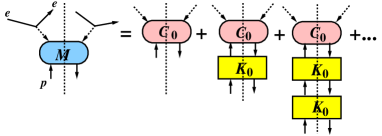
Refer to caption
Figure 1: Raw factorization theorem in the physical gauge.

Factorization scheme of EGMPR [3], see Fig. 1, was customized to MS¯¯𝑀𝑆\overline{MS} by CFP [2]:

F=C011K0=C(α,Q2μ2)Γ(α,1ϵ),Γ(α,1ϵ)(11K)=1+K+KK+KKK+,K=K011(1)K0,C=C011(1)K0,\begin{split}F&=C_{0}\cdot\frac{1}{1-K_{0}}=C\left(\alpha,\frac{Q^{2}}{\mu^{2}}\right)\otimes\Gamma\left(\alpha,\frac{1}{\epsilon}\right),\\ \Gamma&\left(\alpha,\frac{1}{\epsilon}\right)\equiv\left(\frac{1}{1-K}\right)_{\otimes}=1+K+K\otimes K+K\otimes K\otimes K+...,\\ K&=\mathbbm{P}K_{0}\cdot\frac{1}{1-(1-\mathbbm{P})\cdot K_{0}},\quad C=C_{0}\cdot\frac{1}{1-(1-\mathbbm{P})\cdot K_{0}},\end{split} (1)

where the ladder part ΓΓ\Gamma corresponds to MC parton shower and C𝐶C is the hard process part 333 Multiplication symbol \cdot means full phase space integration dnksuperscript𝑑𝑛𝑘d^{n}k while convolution tensor-product\otimes only the integration over the 1-dim. lightcone variable.. NLO kernels were extracted in ref. [2] from the coefficient of a single pole 1ϵ1italic-ϵ\frac{1}{\epsilon} in ΓΓ\Gamma. Projection operator of CFP, =PspinPkinPP,subscript𝑃𝑠𝑝𝑖𝑛subscript𝑃𝑘𝑖𝑛𝑃𝑃\mathbbm{P}=P_{spin}\;P_{kin}\;PP, consists of the kinematic (on-shell) projection operator Pkinsubscript𝑃𝑘𝑖𝑛P_{kin}, spin projection operator Pspinsubscript𝑃𝑠𝑝𝑖𝑛P_{spin} and PP𝑃𝑃PP extracting pole part 1ϵk,k>01superscriptitalic-ϵ𝑘𝑘0\frac{1}{\epsilon^{k}},k>0.

In our MC solutions we use the standard interpretation [11] of the collinear ϵitalic-ϵ\epsilon-poles:

1ε=0μFdkTkT(kTμF)ϵ.1𝜀superscriptsubscript0subscript𝜇𝐹𝑑superscript𝑘𝑇superscript𝑘𝑇superscriptsuperscript𝑘𝑇subscript𝜇𝐹italic-ϵ\frac{1}{\varepsilon}=\int_{0}^{\mu_{F}}\frac{dk^{T}}{k^{T}}\;\left(\frac{k^{T}}{\mu_{F}}\right)^{\epsilon}. (2)

However, the ladder part in CFP/EGMPR scheme features enormous cancellations, as can be seen already at the LO level444Omitting for simplicity 1/ϵn1superscriptitalic-ϵ𝑛1/\epsilon^{n} poles due to running of the coupling constant from the consideration.:

Γ11(1e1ε)=1+(1e1ε)+(1e1ε)2+,similar-to-or-equalsΓ111superscript𝑒1𝜀11superscript𝑒1𝜀superscript1superscript𝑒1𝜀2\Gamma\simeq\frac{1}{1-\Big{(}1-e^{-\frac{1}{\varepsilon}}\Big{)}}=1+\Big{(}1-e^{-\frac{1}{\varepsilon}}\Big{)}+\Big{(}1-e^{-\frac{1}{\varepsilon}}\Big{)}^{2}+..., (3)

while from RGE and explicit LO calculation we obtain readily Γ=e+1ε=1+1ε+12!1ε2+Γsuperscript𝑒1𝜀11𝜀121superscript𝜀2\Gamma=e^{+\frac{1}{\varepsilon}}=1+\frac{1}{\varepsilon}+\frac{1}{2!}\frac{1}{\varepsilon^{2}}+... In the MC we need this exponent manifestly, if possible directly from the Feynman diagrams!

The above exponential nature of the QCD evolution of PDFs is manifest in the following master formula

F=C011K0=C0μ[K0]expTO({K0ss[K0]})μ,μ(K0)=𝔹μ[11K0]1+𝔹μ[K0]+𝔹μ[K0K0]+𝔹μ[K0K0K0]+\begin{split}&F=C_{0}\cdot\frac{1}{1-K_{0}}=C_{0}\cdot\overleftarrow{\mathbbm{R}}_{\mu}[K_{0}]\cdot\exp_{TO}\left(\overleftarrow{\mathbbm{P}}^{\prime}\left\{{}^{s}K_{0}\cdot\overleftarrow{\mathbbm{R}}_{s}[K_{0}]\right\}\right)_{\mu},\\ &\overleftarrow{\mathbbm{R}}_{\mu}(K_{0})=\overleftarrow{\mathbbm{B}}_{\mu}\left[\frac{1}{1-K_{0}}\right]\equiv 1+\overleftarrow{\mathbbm{B}}_{\mu}[K_{0}]+\overleftarrow{\mathbbm{B}}_{\mu}[K_{0}\cdot K_{0}]+\overleftarrow{\mathbbm{B}}_{\mu}[K_{0}\cdot K_{0}\cdot K_{0}]+\dots\end{split} (4)

which is serving as a generating functional of the exclusive parton distributions implemented in the MC. Here, expTOsubscript𝑇𝑂\exp_{TO} is the time ordered exponential in the time evolution variable t=lnμ𝑡𝜇t=\ln\mu, where μ𝜇\mu is factorization scale variable. Operator 𝔹𝔹\overleftarrow{\mathbbm{B}} is defined recursively555 Similarly as β𝛽\beta-functions in Yennie-Frautschi-Suura[12] subtraction scheme. See also [13].:

𝔹μ[K0]=K0μ{sK0},𝔹μ[K0K0]=K0K0μ{s2K0}s2{s1K0}μ{s2K0𝔹s2[K0]}𝔹μ[K0]μ{K0},𝔹μ[K0K0K0]=K0K0K0μ{s3K0}s3{s2K0}s2{s1K0}\begin{split}&\overleftarrow{\mathbbm{B}}_{\mu}[K_{0}]=K_{0}-\mathbbm{P}^{\prime}_{\mu}\{^{s}K_{0}\},\\ &\overleftarrow{\mathbbm{B}}_{\mu}[K_{0}\cdot K_{0}]\!=\!K_{0}\cdot K_{0}\!-\mathbbm{P}^{\prime}_{\mu}\{^{s_{2}}K_{0}\}\!\cdot\mathbbm{P}^{\prime}_{s_{2}}\{^{s_{1}}K_{0}\}\!-\mathbbm{P}^{\prime}_{\mu}\{^{s_{2}}K_{0}\!\cdot\overleftarrow{\mathbbm{B}}_{s_{2}}[K_{0}]\}\!-\overleftarrow{\mathbbm{B}}_{\mu}[K_{0}]\!\cdot\mathbbm{P}^{\prime}_{\mu}\{K_{0}\},\\ &\overleftarrow{\mathbbm{B}}_{\mu}[K_{0}\cdot K_{0}\cdot K_{0}]=K_{0}\cdot K_{0}\cdot K_{0}-\mathbbm{P}^{\prime}_{\mu}\{^{s_{3}}K_{0}\}\cdot\mathbbm{P}^{\prime}_{s_{3}}\{^{s_{2}}K_{0}\}\cdot\mathbbm{P}^{\prime}_{s_{2}}\{^{s_{1}}K_{0}\}-\dots\end{split} (5)

More terms in the recursion can be obtained by expanding LHS and RHS of eq. (4) in powers of K0subscript𝐾0K_{0} and using definition of expTOsubscript𝑇𝑂\exp_{TO} (see below). The key point is the definition of modified projection operator superscript\overleftarrow{\mathbbm{P}}^{\prime}: (a) it does spin projection as \mathbbm{P} of CFP, (b) it sets its incoming momentum on-shell in the part of the diagram towards the hard process, (c) it acts on the integrand of the Lorentz invariant phase space (LIPS), before integration, (d) it sets upper limit μ𝜇\mu on the phase space for all its own real (cut) partons, eg. μ>s(k1,..,kn)=max(kiT)\mu>s(k_{1},..,k_{n})=\max(k^{T}_{i}), (e) our preferred choice is rapidity ordering choice; s(k1,..,kn)=a(k1,..,kn)=max(kiT/αi)s(k_{1},..,k_{n})=a(k_{1},..,k_{n})=\max(k^{T}_{i}/\alpha_{i}), αi=ki+/Esubscript𝛼𝑖subscriptsuperscript𝑘𝑖𝐸\alpha_{i}=k^{+}_{i}/E, (f) μ(A)subscriptsuperscript𝜇𝐴\overleftarrow{\mathbbm{P}}^{\prime}_{\mu}(A) acts on A𝐴A which is at most single-log (collinear) divergent and extracts this singularity from the LIPS integrand666For instance by rescaling all kiTλkiTsubscriptsuperscript𝑘𝑇𝑖𝜆subscriptsuperscript𝑘𝑇𝑖k^{T}_{i}\to\lambda k^{T}_{i} and taking coefficient in front of 1/λ1𝜆1/\lambda term., (g) μ(K0)subscriptsuperscript𝜇subscript𝐾0\overleftarrow{\mathbbm{P}}^{\prime}_{\mu}(K_{0}) is legal, as K0subscript𝐾0K_{0} is single-log divergent, (h) nesting like [K0(1(K0))]superscriptdelimited-[]subscript𝐾01superscriptsubscript𝐾0\overleftarrow{\mathbbm{P}}^{\prime}[K_{0}\cdot(1-\overleftarrow{\mathbbm{P}}^{\prime}(K_{0}))] is allowed, as long as its argument is no more than single-log divergent, (e) superscript\overleftarrow{\mathbbm{P}}^{\prime} does not include PP operation. Finally, the time ordered exponential reads:

expTO(μ{A})μ=1+μ{A}+μ{s2A}s2{s1A}+μ{s3A}s3{s2A}s2{s1A}+\exp_{TO}\left(\mathbbm{P}^{\prime}_{\mu}\{A\}\right)_{\mu}\!=\!1+\mathbbm{P}^{\prime}_{\mu}\{A\}+\mathbbm{P}^{\prime}_{\mu}\{^{s_{2}}A\}\cdot\mathbbm{P}^{\prime}_{s_{2}}\{^{s_{1}}A\}+\mathbbm{P}^{\prime}_{\mu}\{^{s_{3}}A\}\cdot\mathbbm{P}^{\prime}_{s_{3}}\{^{s_{2}}A\}\cdot\mathbbm{P}^{\prime}_{s_{2}}\{^{s_{1}}A\}+\dots (6)

where notation {sA}\{^{s}A\} means that s=a(a1,,an)=max(a1,,an)𝑠𝑎subscript𝑎1subscript𝑎𝑛subscript𝑎1subscript𝑎𝑛s=a(a_{1},...,a_{n})=\max(a_{1},...,a_{n}). For instance for n=3𝑛3n=3 the entire integrand multiplied by θμ>s3>s2>s1subscript𝜃𝜇subscript𝑠3subscript𝑠2subscript𝑠1\theta_{\mu>s_{3}>s_{2}>s_{1}}. Variable μ𝜇\mu is constant, while sisubscript𝑠𝑖s_{i} depend on the 4-momenta integration variables.

Master formula of eq. (4) is very important for us, as it serves as a generating functional of the exclusive distributions beyond LO implemented in the MC. In CFP scheme the time ordered exponential is present for the inclusive PDFs, and results from the renormalization group equations, not directly from Feynman diagrams. Deriving eq. (4) directly from diagrams at any perturbative order remains an open important problem777In particular the effect of the running coupling costant deserves careful discussion.. For the time being we check order by order that: (i) at the inclusive level we maintain full compability with the CFP scheme, (ii) we reproduce fixed order matrix squared element times LIPS results wherever possible and/or necessary.

From now on, in the factorization formula (4), we focus on the exclusive PDF (ePDF) 𝒟(μ,k1,,kn)𝒟𝜇subscript𝑘1subscript𝑘𝑛\mathcal{D}(\mu,k_{1},...,k_{n}), which is the integrand of the inclusive PDF:

D(μ)=expTO({K0ss[K0]})(μ)=expTO(K),𝐷𝜇subscript𝑇𝑂superscriptsuperscriptsubscript𝐾0𝑠subscript𝑠delimited-[]subscript𝐾0𝜇subscript𝑇𝑂𝐾D(\mu)=\exp_{TO}\left(\overleftarrow{\mathbbm{P}}^{\prime}\left\{{}^{s}K_{0}\cdot\overleftarrow{\mathbbm{R}}_{s}[K_{0}]\right\}\right)(\mu)=\exp_{TO}(K), (7)

The x𝑥x-dependent PDFs (inclusive) are obtained by means of inserting δ(xx(k1,,kn))𝛿𝑥𝑥subscript𝑘1subscript𝑘𝑛\delta(x-x(k_{1},...,k_{n})) in the integrand 888Such an insertion we shall often mark as ()xsubscript𝑥(...)_{x}. In the MC it means histogramming of x𝑥x. It also helps eliminating x=0𝑥0x=0 from the consideration., D(μ)D(μ,x)=D(μ)x𝐷𝜇𝐷𝜇𝑥𝐷subscript𝜇𝑥D(\mu)\to D(\mu,x)=D(\mu)_{x}.

The standard inclusive PDF, D(μ,x)=𝑑Lips𝒟(μ,k1,,kn,x)𝐷𝜇𝑥differential-dLips𝒟𝜇subscript𝑘1subscript𝑘𝑛𝑥D(\mu,x)=\int d{\rm Lips}\;\mathcal{D}(\mu,k_{1},...,k_{n},x), is obtained form ePDF by the phase space integration. It obeys by construction the ordinary evolution equation

μD(μ,x)=𝒫D(μ,x)subscript𝜇𝐷𝜇𝑥tensor-product𝒫𝐷𝜇𝑥\partial_{\mu}D(\mu,x)=\mathcal{P}\otimes D(\mu,x) (8)

with the inclusive DGLAP kernel

𝒫(x)=ln(μ)(Kμ)x=𝑑Lipsδ(xki+E0)δ(1sμ)ddLipsμ{K0ss[K0]}.𝒫𝑥𝜇subscriptsubscript𝐾𝜇𝑥differential-dLips𝛿𝑥superscriptsubscript𝑘𝑖subscript𝐸0𝛿1𝑠𝜇𝑑𝑑Lipssubscriptsuperscript𝜇superscriptsubscript𝐾0𝑠subscript𝑠delimited-[]subscript𝐾0\begin{split}\mathcal{P}(x)&=\frac{\partial}{\partial\ln(\mu)}(K_{\mu})_{x}\;=\int\!\!d{\rm Lips}\;\delta\bigg{(}x-\frac{\sum k_{i}^{+}}{E_{0}}\bigg{)}\;\delta\left(1-\frac{s}{\mu}\right)\frac{d}{d{\rm Lips}}\overleftarrow{\mathbbm{P}}^{\prime}_{\mu}\left\{{}^{s}K_{0}\cdot\overleftarrow{\mathbbm{R}}_{s}[K_{0}]\right\}.\end{split} (9)

The LO and NLO truncations of the evolution kernel Kμsubscript𝐾𝜇K_{\mu} are: KμLO=μ{K0s}subscriptsuperscript𝐾𝐿𝑂𝜇subscriptsuperscript𝜇superscriptsubscript𝐾0𝑠K^{LO}_{\mu}=\overleftarrow{\mathbbm{P}}^{\prime}_{\mu}\left\{{}^{s}K_{0}\right\}, taken at 𝒪(α1)𝒪superscript𝛼1{\cal O}(\alpha^{1}) and KμNLO=μ{(K0+K0(1)K0)s}K^{NLO}_{\mu}=\overleftarrow{\mathbbm{P}}^{\prime}_{\mu}\left\{{}^{s}\big{(}K_{0}+K_{0}\cdot(1-\overleftarrow{\mathbbm{P}}^{\prime})\cdot K_{0}\big{)}\right\}, truncated at 𝒪(α2)𝒪superscript𝛼2{\cal O}(\alpha^{2}). The 2PI kernel K0subscript𝐾0K_{0} of CFP scheme (non-singlet bremsstrahlung) at LO+NLO is:

K0=2([Uncaptioned image])+[Uncaptioned image]+  2([Uncaptioned image])+[Uncaptioned image],subscript𝐾02[Uncaptioned image]+[Uncaptioned image]+2[Uncaptioned image]+[Uncaptioned image]K_{0}=2\Re\bigg{(}\raisebox{-11.0pt}{\includegraphics[height=31.29802pt]{xBrem1v.pdf}}\bigg{)}\hbox{\LARGE+}\;\;\raisebox{-11.0pt}{\includegraphics[height=31.29802pt]{xBrem1r.pdf}}\;\;\hbox{\LARGE+}\;\;2\Re\bigg{(}\raisebox{-11.0pt}{\includegraphics[height=31.29802pt]{xBrem2v.pdf}}\bigg{)}\hbox{\LARGE+}\;\;\raisebox{-12.0pt}{\includegraphics[height=34.1433pt]{xBremXr.pdf}}, (10)

where dashed lines are gluons, blobs marked “Virt” may include several (one loop) subgraphs. First two terms in the x𝑥x-dependent T.O. exponential with LO kernel read

expTO(Q{KLO})xδx=1+Q{K0LO}x=δx=1+2([Uncaptioned image])x+([Uncaptioned image])x=δx=1+lnQq02CFαsπ(1+x22(1x))+=δx=1+lnQq0𝒫qq(x),\begin{split}&\exp_{TO}\left(\mathbbm{P}^{\prime}_{Q}\{K^{LO}\}\right)_{x}\simeq\delta_{x=1}+\mathbbm{P}^{\prime}_{Q}\{K_{0}^{LO}\}_{x}=\hbox{\large$\delta_{x=1}+$}2\Re\bigg{(}\raisebox{-11.0pt}{\includegraphics[height=31.29802pt]{xBrem1vP.pdf}}\bigg{)}_{x}\hbox{\Large+}\bigg{(}\raisebox{-11.0pt}{\includegraphics[height=31.29802pt]{xBrem1rP.pdf}}\bigg{)}_{x}\\ &~{}~{}~{}~{}~{}~{}~{}~{}=\delta_{x=1}+\ln\frac{Q}{q_{0}}\;\frac{2C_{F}\alpha_{s}}{\pi}\left(\frac{1+x^{2}}{2(1-x)}\right)_{+}=\delta_{x=1}+\ln\frac{Q}{q_{0}}\;\mathcal{P}_{qq}(x),\end{split} (11)

where q0subscript𝑞0q_{0} is IR cut-off and 𝒫qq(x)=2CFαsπ(1+x22(1x))+subscript𝒫𝑞𝑞𝑥2subscript𝐶𝐹subscript𝛼𝑠𝜋subscript1superscript𝑥221𝑥\mathcal{P}_{qq}(x)=\frac{2C_{F}\alpha_{s}}{\pi}\left(\frac{1+x^{2}}{2(1-x)}\right)_{+}.

The LO exclusive distribution999Here δ𝛿\delta is another IR cut-off parameter, the same as in CFP. ρ¯B1r=2CFαsπ21+(1α1)221𝐤12θα1>δsubscript¯𝜌𝐵1𝑟2subscript𝐶𝐹subscript𝛼𝑠superscript𝜋21superscript1subscript𝛼1221superscriptsubscript𝐤12subscript𝜃subscript𝛼1𝛿\bar{\rho}_{B1r}=\frac{2C_{F}\alpha_{s}}{\pi^{2}}\;\frac{1+(1-\alpha_{1})^{2}}{2}\;\frac{1}{{\bf{k}}_{1}^{2}}\theta_{\alpha_{1}>\delta} resides inside

[Uncaptioned image]=d3k12k10θQ>a1>q0ρ¯B1r(k1)=α1𝑑α1d2𝐚1𝑑ϕ1θQ>a1>q0ρ¯B1r(k1),[Uncaptioned image]superscript𝑑3subscript𝑘12superscriptsubscript𝑘10subscript𝜃𝑄subscript𝑎1subscript𝑞0subscript¯𝜌𝐵1𝑟subscript𝑘1subscript𝛼1differential-dsubscript𝛼1superscript𝑑2subscript𝐚1differential-dsubscriptitalic-ϕ1subscript𝜃𝑄subscript𝑎1subscript𝑞0subscript¯𝜌𝐵1𝑟subscript𝑘1\begin{split}&\raisebox{-11.0pt}{\includegraphics[height=31.29802pt]{xBrem1rP.pdf}}=\int\frac{d^{3}k_{1}}{2k_{1}^{0}}\;\theta_{Q>a_{1}>q_{0}}\;\bar{\rho}_{B1r}(k_{1})=\int\alpha_{1}d\alpha_{1}d^{2}{\bf{a}}_{1}d\phi_{1}\;\theta_{Q>a_{1}>q_{0}}\;\bar{\rho}_{B1r}(k_{1}),\end{split} (12)

where 𝐚i𝐤1/α1subscript𝐚𝑖subscript𝐤1subscript𝛼1{\bf{a}}_{i}\equiv{\bf{k}}_{1}/\alpha_{1} and a1=|𝐚1|subscript𝑎1subscript𝐚1a_{1}=|{\bf{a}}_{1}| similar-to-or-equals\simeq polar angle of the gluon with transverse momentum 𝐤1subscript𝐤1{\bf{k}}_{1}. The trivial phase space integration gives Sudakov double log or LO kernel:

[Uncaptioned image]=2CFαsπlnQq0(ln1δ34)=SISR,([Uncaptioned image])x=lnQq0𝒫qq(x)θ1x<ϵ.formulae-sequence[Uncaptioned image]2subscript𝐶𝐹subscript𝛼𝑠𝜋𝑄subscript𝑞01𝛿34subscript𝑆ISRsubscript[Uncaptioned image]𝑥𝑄subscript𝑞0subscript𝒫𝑞𝑞𝑥subscript𝜃1𝑥italic-ϵ\raisebox{-11.0pt}{\includegraphics[height=31.29802pt]{xBrem1rP.pdf}}=\frac{2C_{F}\alpha_{s}}{\pi}\ln\frac{Q}{q_{0}}\left(\ln\frac{1}{\delta}-\frac{3}{4}\right)=S_{{}_{\rm ISR}},\quad\quad\quad\bigg{(}\raisebox{-11.0pt}{\includegraphics[height=31.29802pt]{xBrem1rP.pdf}}\bigg{)}_{x}=\ln\frac{Q}{q_{0}}\;\mathcal{P}_{qq}(x)\theta_{1-x<\epsilon}. (13)

In the TO exponential D(Q)=expTO(Q{KLO})𝐷𝑄subscript𝑇𝑂subscriptsuperscript𝑄superscript𝐾𝐿𝑂D(Q)=\exp_{TO}\big{(}\mathbbm{P}^{\prime}_{Q}\{K^{LO}\}\big{)} the virtual contribution  [Uncaptioned image]=SISRabsentsubscript𝑆𝐼𝑆𝑅=-S_{ISR} factorizes off:

D(Q)=1+Q{K0}+Q{s2K0}s2{s1K0}+Q{s3K0}s3{s2K0}s2{s1K0}+=exp([Uncaptioned image]){[Uncaptioned image]+[Uncaptioned image]+[Uncaptioned image]+[Uncaptioned image]+…}=eSISR{1+n=1j=1nd3kj2kj0Π(kj)ρ¯B1LO(kj)θaj>aj1}=eSISR{e+SISR}=1.\begin{split}&D(Q)\!=1+\mathbbm{P}^{\prime}_{Q}\{K_{0}\}+\mathbbm{P}^{\prime}_{Q}\{^{s_{2}}K_{0}\}\cdot\mathbbm{P}^{\prime}_{s_{2}}\{^{s_{1}}K_{0}\}+\mathbbm{P}^{\prime}_{Q}\{^{s_{3}}K_{0}\}\cdot\mathbbm{P}^{\prime}_{s_{3}}\{^{s_{2}}K_{0}\}\cdot\mathbbm{P}^{\prime}_{s_{2}}\{^{s_{1}}K_{0}\}+...\\ &=\exp\left(\Re\;\raisebox{-10.0pt}{\includegraphics[height=28.45274pt]{xBrem1vP.pdf}}\right)\;\left\{\raisebox{-10.0pt}{\includegraphics[height=28.45274pt]{xBorn.pdf}}\hbox{\LARGE+}\;\;\raisebox{-10.0pt}{\includegraphics[height=28.45274pt]{xBrem1rP.pdf}}\hbox{\LARGE+}\;\;\raisebox{-10.0pt}{\includegraphics[height=28.45274pt]{xB2P1P}}\hbox{\LARGE+}\;\;\raisebox{-12.0pt}{\includegraphics[height=31.29802pt]{xB321P.pdf}}\hbox{\LARGE+...}\right\}\\ &=e^{-S_{{}_{\rm ISR}}}\bigg{\{}1+\sum_{n=1}^{\infty}\prod_{j=1}^{n}\int\frac{d^{3}k_{j}}{2k_{j}^{0}}\;\Pi(k_{j})\;\bar{\rho}_{B1}^{LO}(k_{j})\theta_{a_{j}>a_{j-1}}\bigg{\}}=e^{-S_{{}_{\rm ISR}}}\;\left\{e^{+S_{{}_{\rm ISR}}}\right\}=1.\end{split} (14)

The x𝑥x-dependent version of the same D(Q,x)=expTO(Q{KLO})xD(Q,x)=\exp_{TO}\bigg{(}\mathbbm{P}^{\prime}_{Q}\{K^{LO}\}\bigg{)}_{x} reads

D(x,Q)=eSISR{δx=1+n=1(j=1nqj1Qdajaj01δ𝑑zj02πdφj2π𝒫qqθ(zj))δx=izi}.𝐷𝑥𝑄superscript𝑒subscript𝑆ISRsubscript𝛿𝑥1superscriptsubscript𝑛1superscriptsubscriptproduct𝑗1𝑛superscriptsubscriptsubscript𝑞𝑗1𝑄𝑑subscript𝑎𝑗subscript𝑎𝑗superscriptsubscript01𝛿differential-dsubscript𝑧𝑗superscriptsubscript02𝜋𝑑subscript𝜑𝑗2𝜋subscriptsuperscript𝒫𝜃𝑞𝑞subscript𝑧𝑗subscript𝛿𝑥subscriptproduct𝑖subscript𝑧𝑖D(x,Q)=e^{-S_{{}_{\rm ISR}}}\bigg{\{}\delta_{x=1}+\sum_{n=1}^{\infty}\bigg{(}\prod_{j=1}^{n}\;\int_{q_{j-1}}^{Q}\frac{da_{j}}{a_{j}}\int_{0}^{1-\delta}dz_{j}\int_{0}^{2\pi}\frac{d\varphi_{j}}{2\pi}\;\mathcal{P}^{\theta}_{qq}(z_{j})\bigg{)}\delta_{x=\prod_{i}z_{i}}\bigg{\}}. (15)

From now on we enter NLO world. The NLO kernelKμNLO=μ{(K0+K0(1)K0)s}K^{NLO}_{\mu}=\overleftarrow{\mathbbm{P}}^{\prime}_{\mu}\left\{{}^{s}\big{(}K_{0}+K_{0}\cdot(1-\overleftarrow{\mathbbm{P}}^{\prime})\cdot K_{0}\big{)}\right\} with K0subscript𝐾0K_{0} of eq. (10) (nonsinglet bremsstrahlung) is inserted into T.O. exponent of the NLO ePFD:

DB[1](Q)=exp(SISR[1])(1+Q{Kr}+Q{a2Kr}a2{a1Kr}++Q{a3Kr}a3{a2Kr}a2{a1Kr}+)=exp([Uncaptioned image]){[Uncaptioned image]+[Uncaptioned image]+[Uncaptioned image]+[Uncaptioned image]+…}.\begin{split}&D^{[1]}_{B}(Q)=\exp(-S^{[1]}_{{}_{ISR}})\Big{(}1+\mathbbm{P}^{\prime}_{Q}\{K^{r}\}+\mathbbm{P}^{\prime}_{Q}\{^{a_{2}}K^{r}\}\cdot\mathbbm{P}^{\prime}_{a_{2}}\{^{a_{1}}K^{r}\}+\\ &~{}~{}~{}~{}~{}~{}~{}~{}~{}~{}~{}~{}~{}~{}~{}~{}~{}~{}~{}~{}~{}~{}~{}~{}~{}~{}~{}~{}~{}~{}~{}~{}~{}~{}~{}~{}~{}~{}~{}~{}~{}+\mathbbm{P}^{\prime}_{Q}\{^{a_{3}}K^{r}\}\cdot\mathbbm{P}^{\prime}_{a_{3}}\{^{a_{2}}K^{r}\}\cdot\mathbbm{P}^{\prime}_{a_{2}}\{^{a_{1}}K^{r}\}+\dots\Big{)}\\ &~{}=\exp\left(\Re\raisebox{-8.0pt}{\includegraphics[height=22.76219pt]{xBrem2vvP.pdf}}\right)\Bigg{\{}\raisebox{-9.0pt}{\includegraphics[height=25.60747pt]{xBorn.pdf}}\hbox{\LARGE+}\raisebox{-9.0pt}{\includegraphics[height=25.60747pt]{xKlad1.pdf}}\hbox{\LARGE+}\raisebox{-9.0pt}{\includegraphics[height=25.60747pt]{xKlad2.pdf}}\hbox{\LARGE+}\;\;\;\raisebox{-12.0pt}{\includegraphics[height=34.1433pt]{xKlad3.pdf}}\hbox{\LARGE+...}\Bigg{\}}.\end{split} (16)

Where the zero-real-emission part of the kernel SISR[1]=subscriptsuperscript𝑆delimited-[]1𝐼𝑆𝑅absent-S^{[1]}_{ISR}=[Uncaptioned image] (wave function renormalization up to second order) factorizes and exponentiates.

The remaining part of the NLO kernel Kr=[Uncaptioned image][Uncaptioned image]+[Uncaptioned image]superscript𝐾𝑟[Uncaptioned image][Uncaptioned image]+[Uncaptioned image]K^{r}=\raisebox{-9.0pt}{\includegraphics[height=25.60747pt]{xKlad1.pdf}}\;\hbox{\LARGE$\equiv$}\;\;\raisebox{-9.0pt}{\includegraphics[height=25.60747pt]{xKseg1vP.pdf}}\;\hbox{\LARGE+}\;\raisebox{-9.0pt}{\includegraphics[height=25.60747pt]{xKseg2rP.pdf}} consists of the one-real-emission part including NLO virtual one loop corrections K1r=[Uncaptioned image][Uncaptioned image]+  2[Uncaptioned image]superscript𝐾1𝑟[Uncaptioned image][Uncaptioned image]+2[Uncaptioned image]K^{1r}=\raisebox{-9.0pt}{\includegraphics[height=25.60747pt]{xKseg1vP.pdf}}\;\hbox{\LARGE$\equiv$}\;\raisebox{-9.0pt}{\includegraphics[height=25.60747pt]{xBrem1rP.pdf}}\;\hbox{\LARGE+}\;\;2\Re\;\raisebox{-9.0pt}{\includegraphics[height=25.60747pt]{xBrem2vP.pdf}} and the pure two-real emission part K2r=[Uncaptioned image][Uncaptioned image]+{[Uncaptioned image]-[Uncaptioned image]}superscript𝐾2𝑟[Uncaptioned image][Uncaptioned image]+[Uncaptioned image]-[Uncaptioned image]K^{2r}=\raisebox{-9.0pt}{\includegraphics[height=25.60747pt]{xKseg2rPink.pdf}}\hbox{\LARGE$\equiv$}\;\raisebox{-9.0pt}{\includegraphics[height=25.60747pt]{xBremXrP.pdf}}\hbox{\LARGE+}\;\Bigg{\{}\raisebox{-9.0pt}{\includegraphics[height=25.60747pt]{xB21P}}\;\hbox{\LARGE-}\;\raisebox{-9.0pt}{\includegraphics[height=25.60747pt]{xB2P1P}}\Bigg{\}}. Eq. (16) could be used directly in the MC, if both K1rsuperscript𝐾1𝑟K^{1r} and K2rsuperscript𝐾2𝑟K^{2r} were positive. Since K2rsuperscript𝐾2𝑟K^{2r} is non-positive we have to recombine K2rsuperscript𝐾2𝑟K^{2r} with 2 real emission distribution, that is to put it back where it came from (reversing what the factorization did):

DB[1](Q)=eSISR[1]{1+[Uncaptioned image]+[Uncaptioned image]+[Uncaptioned image]+[Uncaptioned image]+…+[Uncaptioned image]+[Uncaptioned image]+[Uncaptioned image]+[Uncaptioned image]+…+[Uncaptioned image]+…}.subscriptsuperscript𝐷delimited-[]1𝐵𝑄superscript𝑒subscriptsuperscript𝑆delimited-[]1𝐼𝑆𝑅1+[Uncaptioned image]+[Uncaptioned image]+[Uncaptioned image]+[Uncaptioned image]+…+[Uncaptioned image]+[Uncaptioned image]+[Uncaptioned image]+[Uncaptioned image]+…+[Uncaptioned image]+…\begin{split}&D^{[1]}_{B}(Q)=e^{-S^{[1]}_{{}_{ISR}}}\Bigg{\{}\hbox{\large 1+}\;\raisebox{-7.0pt}{\includegraphics[height=19.91692pt]{xKseg1vP.pdf}}\hbox{\Large+}\raisebox{-8.0pt}{\includegraphics[height=22.76219pt]{xKK.pdf}}\hbox{\Large+}\raisebox{-9.0pt}{\includegraphics[height=25.60747pt]{xKKK.pdf}}\hbox{\Large+}\raisebox{-11.0pt}{\includegraphics[height=31.29802pt]{xKKKK.pdf}}\hbox{\Large+...}\\ &~{}~{}~{}~{}~{}~{}~{}~{}~{}~{}~{}~{}~{}~{}~{}~{}~{}~{}~{}~{}~{}~{}~{}~{}~{}~{}~{}~{}~{}~{}~{}\hbox{\Large+}\raisebox{-8.0pt}{\includegraphics[height=22.76219pt]{xKseg2rPink.pdf}}\hbox{\Large+}\raisebox{-9.0pt}{\includegraphics[height=25.60747pt]{xK2K.pdf}}\hbox{\Large+}\raisebox{-9.0pt}{\includegraphics[height=25.60747pt]{xKK2.pdf}}\hbox{\Large+}\raisebox{-11.0pt}{\includegraphics[height=31.29802pt]{xK2KK.pdf}}\hbox{\Large+...}\hbox{\Large+}\raisebox{-11.0pt}{\includegraphics[height=31.29802pt]{xK2K2.pdf}}\hbox{\Large+...}\Bigg{\}}.\end{split} (17)

In eq. (17) the first row is positive and large (LO + virtual NLO), hence it will go to basic MC, while the second row being small and nonpositive can be absorbed into MC correcting weight. However, it is not so easy to recombine K2rsuperscript𝐾2𝑟K^{2r} with 2 real emissions. The target distribution [Uncaptioned image] + [Uncaptioned image] cannot be implemented in the  (17) by means of MC-reweighting [Uncaptioned image], simply because it is zero outside simplex Q>a2>a1>q0𝑄subscript𝑎2subscript𝑎1subscript𝑞0Q>a_{2}>a_{1}>q_{0}, while the target distribution is nonzero in the bigger rectangle Q>max(a2,a1)>q0𝑄subscript𝑎2subscript𝑎1subscript𝑞0Q>\max(a_{2},a_{1})>q_{0}. Going back to original Feynman diagrams we see that the above problem turns out to be fictitious, if we properly keep track of the Bose-Einstein (BE) symmetrization:

[Uncaptioned image]= 2[Uncaptioned image]+{[Uncaptioned image]-[Uncaptioned image]}+{[Uncaptioned image]-[Uncaptioned image]}=d3k22k20d3k12k10θQ>max(a2,a1)>0θa2>a1(β1B(k2,k1)+β1B(k1,k2)),\begin{split}&\raisebox{-10.0pt}{\includegraphics[height=25.60747pt]{xKseg2rPink.pdf}}\hbox{\LARGE=}\;2\raisebox{-9.0pt}{\includegraphics[height=25.60747pt]{xBremXrP.pdf}}\hbox{\LARGE+}\;\Bigg{\{}\raisebox{-9.0pt}{\includegraphics[height=25.60747pt]{xB21P.pdf}}\;\hbox{\LARGE-}\;\raisebox{-9.0pt}{\includegraphics[height=25.60747pt]{xB2P1P.pdf}}\Bigg{\}}\hbox{\LARGE+}\;\Bigg{\{}\raisebox{-9.0pt}{\includegraphics[height=25.60747pt]{xB12P.pdf}}\hbox{\LARGE-}\;\raisebox{-9.0pt}{\includegraphics[height=25.60747pt]{xB1P2P.pdf}}\Bigg{\}}\\ &~{}~{}~{}~{}~{}~{}~{}~{}~{}~{}~{}~{}=\int\frac{d^{3}k_{2}}{2k_{2}^{0}}\;\int\frac{d^{3}k_{1}}{2k_{1}^{0}}\;\theta_{Q>\max(a_{2},a_{1})>0}\;\theta_{a_{2}>a_{1}}(\beta_{1B}(k_{2},k_{1})+\beta_{1B}(k_{1},k_{2})),\end{split} (18)

where for purely technical reasons we include an internal ordering θa2>a1subscript𝜃subscript𝑎2subscript𝑎1\theta_{a_{2}>a_{1}} for the already symmetric integrand. See ref. [14] for definition of the NLO 2-gluon function β1B(k1,k2)subscript𝛽1𝐵subscript𝑘1subscript𝑘2\beta_{1B}(k_{1},k_{2}).

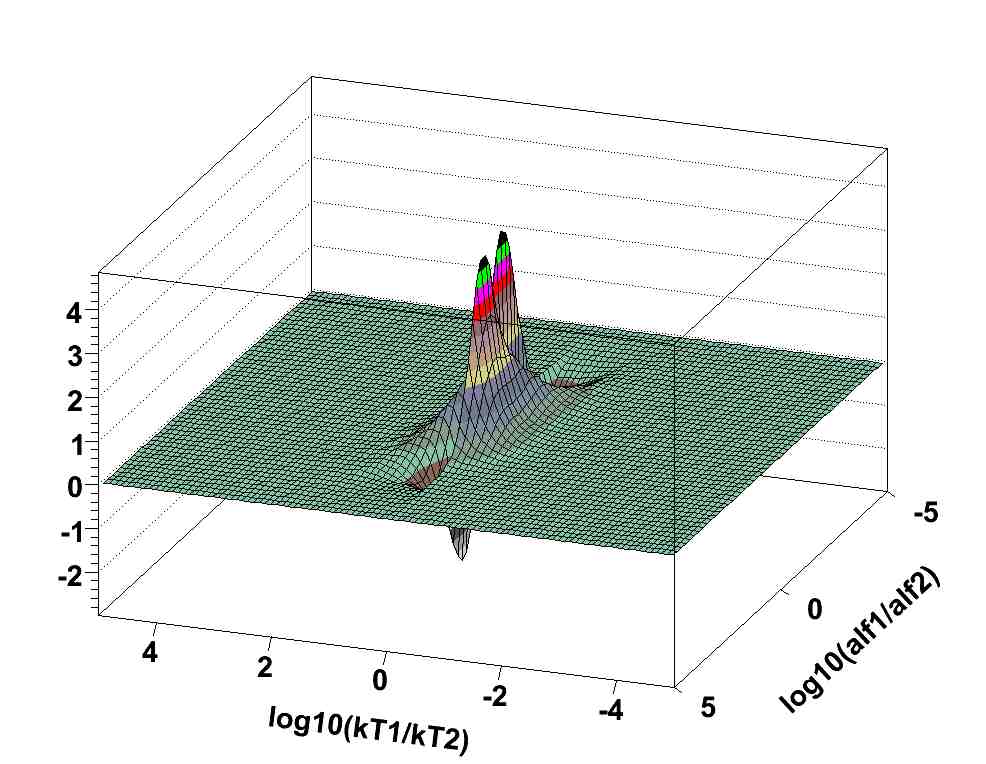
Refer to caption
Figure 2: Two-real-gluon NLO correlation function.

We call sometimes the resulting MC weight the NLO short range correlation function, because it contributes significantly only if both gluons are non-soft and have transverse momenta (or rapidities) almost equal, as seen in the plot of Fig. 2, see [14]. BE symmetrization requires clever reorganization of combinatorics, if want to gain on the computation speed by means of excluding terms equal zero from the BE symmetrization sum. For instance, BE symmetrization over 3!33! permutations of 3 arguments of a single NLO correlation function and one LO spectator distribution reduces to only 2 terms101010For simplicity we are drawing here only of half of the ladder.:

{π}[Uncaptioned image]={π}[Uncaptioned image],subscript𝜋[Uncaptioned image]absentsubscriptsuperscript𝜋[Uncaptioned image]\hbox{\LARGE$\sum\limits_{\{\pi\}}$}\;\;\raisebox{-28.45274pt}{\includegraphics[height=56.9055pt]{xK2Kpi.pdf}}\;\hbox{\LARGE$=\sum\limits_{\{\pi^{\bullet}\}}$}\;\;\raisebox{-28.45274pt}{\includegraphics[height=56.9055pt]{xK2Kbpi.pdf}}\;, (19)

Permutation πksubscript𝜋𝑘\pi_{k} performs the right ordering a(πk)3>a(πk)2>a(πk)3subscript𝑎subscriptsubscript𝜋𝑘3subscript𝑎subscriptsubscript𝜋𝑘2subscript𝑎subscriptsubscript𝜋𝑘3a_{(\pi_{k})_{3}}>a_{(\pi_{k})_{2}}>a_{(\pi_{k})_{3}} at a given phase space point k=(k1,k2,k3)𝑘subscript𝑘1subscript𝑘2subscript𝑘3k=(k_{1},k_{2},k_{3}). This is denoted in the above by {π}={(123),(213)}superscript𝜋123213\{\pi^{\bullet}\}=\{(123),(213)\}, where (123)123(123) is identity and (213)213(213) interchanges (πk)1subscriptsubscript𝜋𝑘1(\pi_{k})_{1} and (πk)2subscriptsubscript𝜋𝑘2(\pi_{k})_{2}. Generalization to double insertion of NLO correlation function in the ladder in a sketchy graphical form is:

ja,jb{πa}{πb}[Uncaptioned image].subscriptsubscript𝑗𝑎subscript𝑗𝑏subscriptsuperscriptsubscript𝜋𝑎subscriptsuperscriptsubscript𝜋𝑏[Uncaptioned image]\hbox{\Large$\sum\limits_{j_{a},j_{b}}\sum\limits_{\{\pi_{a}^{\bullet}\}}\sum\limits_{\{\pi_{b}^{\bullet}\}}$}\;\raisebox{-31.29802pt}{\includegraphics[height=56.9055pt]{xK2K2bpi.pdf}}. (20)

The corresponding algebraic formula of the above NLO ePDF can be found in ref. [14], together with the numerical result of the precision MC test.
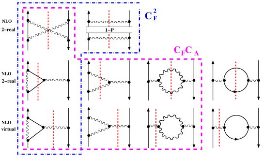
Refer to caption
Figure 3: Feynman diagrams contributing to NLO non-singlet evolution.

So far we have considered the CF2similar-toabsentsuperscriptsubscript𝐶𝐹2\sim C_{F}^{2} diagrams, in Fig. 3. The remaining CFCAsimilar-toabsentsubscript𝐶𝐹subscript𝐶𝐴\sim C_{F}C_{A} diagrams add new problem: strong cancellations between real and virtual contributions in the NLO correction111111 Soft limit of this object was analyzed in ref. [15], exposing colour coherence effects. due to final state radiation (FSR) Sudakov double log, This enforces exponentiation of the FSR already in the LO basic MC, if we aim at positive weight MC events. In the basic MC each gluon in the LO ladder is replaced by resolved multigluon [Uncaptioned image], obtained by iterating/exponentiating “soft counterterm” [Uncaptioned image] in Kfsuperscript𝐾𝑓K^{f}. BE symmetrization is also done for FSR gluons, such that the complete NLO correcting weight includes the following sum:

CF2superscriptsubscript𝐶𝐹2C_{F}^{2}{π}subscriptsuperscript𝜋\sum\limits_{\{\pi^{\bullet}\}}[Uncaptioned image]+CFCAsubscript𝐶𝐹subscript𝐶𝐴+C_{F}C_{A}{π}subscriptsuperscript𝜋\sum\limits_{\{\pi^{\star}\}}[Uncaptioned image] (21)

where Kf=superscript𝐾𝑓absentK^{f}=[Uncaptioned image] is the CFCAsimilar-toabsentsubscript𝐶𝐹subscript𝐶𝐴\sim C_{F}C_{A} component in the above NLO MC weight. Th leading FSR Sudakov double log part is subtracted in Kfsuperscript𝐾𝑓K^{f}. The above sum in the MC weight was already tested for single NLO insertion, giving rise to a well behaved weight distribution. More testing is under way.

Summarizing, we report here on a small but essential part of the larger project, with the aim of implementing NLO DGLAP evolution of the parton distributions in fully unintegrated inclusive form in the Monte Carlo with positive weights (weights equal one). The main result of the ongoing study, so far limited to nonsinglet ePDF, is that this is feasible. Once completed, this project will lead to new type of the parton shower MC for the initial state in LHC and other colliders with hadron beams.

Acknowledgments
Two of the authors (S.J and M.S.) wish to thank Theory Unit of Physics Division, CERN, for generous support during preparation of this work.

References

  • [1] L.N. Lipatov, Sov. J. Nucl. Phys. 20 (1975) 95;
    V.N. Gribov and L.N. Lipatov, Sov. J. Nucl. Phys. 15 (1972) 438;
    G. Altarelli and G. Parisi, Nucl. Phys. 126 (1977) 298;
    Yu. L. Dokshitzer, Sov. Phys. JETP 46 (1977) 64.
  • [2] G. Curci, W. Furmanski, and R. Petronzio, Nucl. Phys. B175 (1980) 27.
  • [3] R. K. Ellis, H. Georgi, M. Machacek, H. D. Politzer, and G. G. Ross, Phys. Lett. B78 (1978) 281.
  • [4] J. C. Collins, D. E. Soper, and G. Sterman, Nucl. Phys. B250 (1985) 199.
  • [5] G. T. Bodwin, Phys. Rev. D31 (1985) 2616.
  • [6] T. Sjostrand, Phys. Lett. B157 (1985) 321.
  • [7] G. Marchesini and B. R. Webber, Nucl. Phys. B310 (1988) 461.
  • [8] H. Tanaka, Prog. Theor. Phys. 110 (2003) 963–973.
  • [9] J. C. Collins and F. Hautmann, JHEP 03 (2001) 016, hep-ph/0009286.
  • [10] J. C. Collins, T. C. Rogers, and A. M. Stasto, Phys. Rev. D77 (2008) 085009, 0708.2833.
  • [11] S. Frixione and B. R. Webber, JHEP 06 (2002) 029, hep-ph/0204244.
  • [12] D. R. Yennie, S. Frautschi, and H. Suura, Ann. Phys. (NY) 13 (1961) 379.
  • [13] J. C. Collins, Phys. Rev. D58 (1998) 094002, hep-ph/9806259.
  • [14] S. Jadach and M. Skrzypek, 0905.1399.
  • [15] M. Slawinska and A. Kusina, 0905.1403.