Intersecting Flavor Branes

Abstract:

We consider an instance of the AdS/CFT duality where the bulk theory contains an open string tachyon, and study the instability from the viewpoint of the boundary field theory. We focus on the specific example of the $AdS_{5}\times S^{5}$ background with two probe $D7$ branes intersecting at general angles. For generic angles supersymmetry is completely broken and there is an open string tachyon between the branes. The field theory action for this system is obtained by coupling to ${\cal N}=4$ super Yang-Mills two ${\cal N}=2$ hyper multiplets in the fundamental representation of the $SU(N)$ gauge group, but with different choices of embedding of the two ${\cal N}=2$ subalgebras into ${\cal N}=4$. On the field theory side we find a one-loop Coleman-Weinberg instability in the effective potential for the fundamental scalars. We identify a mesonic operator as the dual of the open string tachyon. By AdS/CFT, we predict the tachyon mass for small ’t Hooft coupling (large bulk curvature) and confirm that it violates the AdS stability bound.

1 Introduction

Open string tachyon condensation has been studied from many viewpoints, see [1] for a review. Here we consider a holographic (AdS/CFT) setup where the bulk theory contains an open string tachyon, and ask what is the counterpart of tachyon condensation in the boundary field theory. We will identify a sector of the boundary theory as a “holographic open string field theory” capturing the tachyon dynamics. Since the bulk is weakly coupled when the boundary is strongly coupled, and viceversa, we are bound to learn something new from their comparison.

We introduce the open string tachyon by adding to the $AdS_{5}\times S^{5}$ background two probe $D7$ branes intersecting at general angles. Probe branes are the familiar way to include a small number of fundamental flavors in the AdS/CFT correspondence [2]. If the closed string background is supersymmetric, it is possible, and often desirable, to consider configurations of probe branes that preserve some supersymmetry, as e.g. in [2, 3, 4, 5, 6, 7, 8, 9, 10, 11, 12, 13, 14, 15, 16, 17]. Instead, we are after supersymmetry breaking and the ensuing tachyonic instability. Another way to motivate our work is then as a natural susy-breaking generalization of the standard supersymmetric setup of [2]. This generalization is technically challenging, and the technical aspects have some interest of their own. Intersecting brane systems have many other applications in string theory, from string phenomenology to string cosmology, and the technical lessons learnt in our problem may be useful in those contexts as well.

The system that we study is as an open string analogue of the AdS/CFT pairs involving closed string tachyons considered in [18, 19, 20, 21]. Let us briefly review that analysis. In all non-supersymmetric orbifolds of ${\cal N}=4$ SYM, there is an instability for large $N$ and small ’t Hooft coupling $\lambda$. The instability is triggered by the renormalization of double-trace couplings, of the form $f\int d^{4}x\;{\cal O}^{2}$, where ${\cal O}\sim{\rm Tr}X^{2}$ is a scalar bilinear. At leading order for large $N$, the ’t Hooft coupling $\lambda$ is exactly marginal, but the double-trace coupling $f$ runs. The one-loop beta function $\beta_{f}(f,\lambda)\equiv\mu\frac{\partial f}{\partial\mu}$ does not admit zeros for real values of $f$ [19, 20], so conformal invariance is inevitably broken for arbitrarily small (but non-zero) $\lambda$. On the field theory side, the instability can be seen in two equivalent ways. The most direct is as the Coleman-Weinberg instability of the double-trace part of the scalar potential, implying that the scalars $X$ must acquire a non-zero vev. Alternatively [21], we can insist in formally preserving conformal invariance by tuning $f$ to the zero of its beta function, which is a complex number; it then turns out the anomalous dimension $\Delta$ of ${\cal O}$ takes a complex value of the form $\Delta=2+ib\lambda+O(\lambda^{2})$. By AdS/CFT, the bulk scalar field dual to ${\cal O}$ has $m^{2}=\Delta(\Delta-4)=-4-b^{2}\lambda^{2}+O(\lambda^{3})$ (in AdS units), and is thus a “true” tachyon, since its squared mass is below the Breitenlohner-Freedman [22] stability bound $m^{2}_{BF}=-4$. The field theory analysis holds for small ’t Hooft coupling $\lambda$, when the bulk string background is strongly curved and the direct evaluation of its spectrum difficult. By contrast for $\lambda\to\infty$ calculations are easy in the bulk. The bulk analysis reveals that in some cases (orbifolds with fixed points on $S^{5}$) the tachyonic instability persists at large $\lambda$, but it disappears in others (freely acting orbifolds). The upshot is that AdS/CFT makes interesting predictions both at weak and a strong coupling.

The $AdS_{5}\times S^{5}$ background with two probe intersecting $D7$s can be viewed as an open string version of this story. For general angles the bulk theory is unstable via condensation of an open string tachyon, or at least this is the picture for large $\lambda$ where we can calculate the string spectrum. In this paper we focus on the the field theory analysis at small $\lambda$, with the goal of detecting the expected instability.

The first challenge is to write down the Lagrangian of the dual field theory. As is well-known, adding $N_{f}$ parallel $D7$ branes to $AdS_{5}\times S^{5}$ corresponds to adding to ${\cal N}=4$ SYM action $N_{f}$ extra ${\cal N}=2$ hyper multiplet in the fundamental representation of the $SU(N)$ gauge group. The resulting action preserves an ${\cal N}=2$ subalgebra of the original ${\cal N}=4$ supersymmetry algebra – which particular ${\cal N}=2$ being a matter of convention so long as it is the same for all the hyper multiplets. Introducing relative angles between the $D7$ branes corresponds to choosing different embeddings for the ${\cal N}=2$ subalgebras of each different hyper multiplet. In general supersymmetry will be completely broken, while for special angles ${\cal N}=1$ susy is preserved. When ${\cal N}=1$ is preserved we can use ${\cal N}=1$ superspace to write the Lagrangian. When supersymmetry is completely broken the determination of the Lagrangian turns out to be a difficult technical problem that we are unable to solve completely. We cannot fix the quartic terms $\sim Q^{4}$ where $Q$ are the hyper multiplet scalars. The difficulty is related to the lack of an off-shell superspace formulation of ${\cal N}=4$ SYM. Nevertheless, by making what we believe is a mild technical assumption, we can fix the sign of the classical quartic potential. This is sufficient to argue that the theory is indeed unstable from the renormalization of “double-trace” terms $f\int d^{4}x\;{\cal O}^{2}$, where now ${\cal O}\sim\bar{Q}^{\mathfrak{a}}Q_{\mathfrak{a}}$ with $\mathfrak{a}=1,\dots N$ a color index. We are now using “double-trace” in quotes since of course the fields $Q$ are not matrices but vectors, but the logic is much the same. The renormalization of $f$ has the same twofold interpretation as above. We identify the mesonic operator ${\cal O}$ as the dual of the open string tachyon between the two $D7$ branes. The Coleman-Weinberg potential for $Q$ plays the role a holographic effective action for the tachyon.

2 AdS/CFT with Flavor Branes Intersecting at General Angles

We begin with a review the Karch-Katz setup [2], where parallel probe $D7$ branes are used to engineer an ${\cal N}=2$ supersymmetric field theory with flavor. We then break supersymmetry by introducing a relative angle between the $D7$ branes. We derive the dual Lagrangian, up to an ambiguity in the quartic potential for the fundamental scalars. We end the section with a review of the basic bulk-to-boundary dictionary.

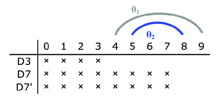
Figure 1: The brane configuration.

2.1 Parallel flavor branes

We start with the familiar $D3/D7$ supersymmetric brane configuration with $N$ “color” $D3$s and $N_{f}$ “flavor” $D7$s, arranged as shown in Figure 1. For now $\theta_{1}=\theta_{2}=0$, that is, all $D7$ branes are parallel to one another. Taking the decoupling limit on the $D3$s wordvolume, the $D3$ branes are replaced by their near-horizon geometry. If $N_{f}\ll N$, we can treat the $D7$ branes as probes in the $AdS_{5}\times S^{5}$ background, neglecting their backreaction [2]. This background preserves ${\cal N}=2$ supersymmetry in four dimensions.

The dual field theory is ${\cal N}=4$ $SU(N)$ SYM coupled to $N_{f}$ ${\cal N}=2$ hyper multiplets in the fundamental representation of the $SU(N)$ color group, arising from the $D3$-$D7$ open strings. We are interested in the case of massless hyper multiplets, corresponding to the brane setup where the $D7$s coincide with the $D3$s (at the origin of the 89 plane). After decoupling, the probe $D7$s fill the whole $AdS_{5}$ and wrap an $S^{3}\subset S^{5}$.

Let us briefly recall the field content of the boundary theory. A more detailed treatment and the full Lagrangian can be found in Appendix A. The ${\cal N}=4$ vector multiplet consists of the gauge field $A_{\mu}$, four Weyl spinors $\lambda^{A}_{\alpha}$, $A=1,\dots,4$ and six real scalars $X_{m}$, $m=4,\dots,9$ corresponding to the six transverse directions to the $D3$ branes. It is convenient to represent the scalars as a self-dual antisymmetric tensor $X^{AB}$ of the $R$-symmetry group $SU(4)_{R}\cong Spin(6)$,

$$(X^{AB})^{\dagger}=\bar{X}_{AB}\equiv\frac{1}{2}\epsilon_{ABCD}\,X^{CD}\,.$$ (1)

The explicit change of variables is

$$X^{AB}=\frac{1}{\sqrt{2}}\left(\begin{array}[]{cc|cc}0&X_{8}+iX_{9}&X_{6}+iX_{7}&X_{4}+iX_{5}\\ -X_{8}-iX_{9}&0&X_{4}-iX_{5}&-X_{6}+iX_{7}\\ \hline\cr-X_{6}-iX_{7}&-X_{4}+iX_{5}&0&X_{8}-iX_{9}\\ -X_{4}-iX_{5}&X_{6}-iX_{7}&-X_{8}+iX_{9}&0\end{array}\right)\,.$$ (2)

Each ${\cal N}=2$ flavor hyper multiplet consists of two Weyl spinors and two complex scalars,

$$\begin{array}[]{ccc}&\psi^{i}_{\alpha}&\\ q^{i}&&\left(\tilde{q}_{i}\right)^{\dagger}\\ &\left(\tilde{\psi}_{i\,\alpha}\right)^{\dagger}&\end{array}$$ (3)

Here $i=1,\dots,N_{f}$ is the flavor index. The scalars form an $SU(2)_{R}$ doublet,

$$Q^{{\cal I}}\equiv\left(\begin{array}[]{c}q\\ \tilde{q}^{\dagger}\end{array}\right)\,,\quad{{\cal I}}=1,2\,.$$ (4)

The flavor hyper multiplets are minimally coupled to the ${\cal N}=2$ vector multiplet that sits inside the ${\cal N}=4$ vector multiplet. This coupling breaks the $R$-symmetry $SU(4)_{R}$ to $SU(2)_{L}\times SU(2)_{R}\times U(1)_{R}$, where $SU(2)_{R}\times U(1)_{R}$ is the $R$-symmetry of the resulting ${\cal N}=2$ theory. There is a certain arbitrariness in the choice of embedding $SU(2)_{L}\times SU(2)_{R}\times U(1)_{R}\subset SU(4)_{R}\cong Spin(6)$. This corresponds to the choice of orientation of the whole stack of $D7$ branes in the 456789 directions (we need to pick an ${\mathbb{R}}^{4}\subset{\mathbb{R}}^{6}$). For example if we choose the configuration of Figure 1, we identify $SU(2)_{L}\times SU(2)_{R}\cong SO(4)$ with rotations in the $4567$ directions and $U(1)_{R}\cong SO(2)$ with a rotation on the $89$ plane. A short calculation using our parametrization of the scalars (2) shows that this corresponds to the following natural embedding of $SU(2)_{L}\times SU(2)_{R}\times U(1)_{R}\subset SU(4)_{R}$:

$$\begin{array}[]{c}1\\ 2\\ 3\\ 4;p[\end{array}\,\left(\begin{array}[]{cc|cc}SU_{R}(2)\times U(1)_{R}&&&\\ &&&\\ \hline\cr&&&\\ &&&SU_{L}(2)\times U(1)_{R}^{*}\end{array}\right)\,.$$ (5)

Of course, any other choice would be equivalent, so long as it is performed simultaneously for all $D7$ branes. With the choice (5), the ${\cal N}=4$ vector multiplet splits into the ${\cal N}=2$ vector multiplet

$$\begin{array}[]{ccc}&A_{\mu}&\\ \lambda^{1}_{\alpha}&&\lambda^{2}_{\alpha}\\ &\frac{X_{8}+iX_{9}}{\sqrt{2}}&\end{array}\,,$$ (6)

and the ${\cal N}=2$ hyper multiplet

$$\begin{array}[]{ccc}&\lambda^{3}_{\alpha}&\\ \frac{X_{4}+iX_{5}}{\sqrt{2}}&&\frac{X_{6}+iX_{7}}{\sqrt{2}}\\ &\lambda^{4}_{\alpha}&\end{array}\,.$$ (7)

The two Weyl spinors in the vector multiplet form an $SU(2)_{R}$ doublet

$$\Lambda_{{\cal I}}\equiv\left(\begin{array}[]{c}\lambda_{1}\\ \lambda_{2}\end{array}\right)\,,\quad{\cal I}=1,2\,,$$ (8)

while the two spinors in the hyper multiplet form an $SU(2)_{L}$ doublet,

$$\hat{\Lambda}_{\hat{\cal I}}\equiv\left(\begin{array}[]{c}\lambda_{3}\\ \lambda_{4}\end{array}\right)\,,\quad\hat{{\cal I}}=1,2\,.$$ (9)

We use ${\cal I}\,,{\cal J}\,\dots=1,2$ for $SU(2)_{R}$ indices and $\hat{\cal I}\,,\hat{\cal J}\,\dots=1,2$ for $SU(2)_{L}$ indices. To make the $SU(2)_{L}\times SU(2)_{R}$ quantum numbers of the scalars more transparent we also introduce the $2\times 2$ complex matrix ${\cal X}_{{\cal I}\hat{\cal I}}$, defined as the off-diagonal block of $X^{AB}$,

$${\cal X}^{\hat{\cal I}{\cal I}}=\left(\begin{array}[]{cc}X_{6}+iX_{7}&X_{4}+iX_{5}\\ X_{4}-iX_{5}&-X_{6}+iX_{7}\end{array}\right)\,.$$ (10)

Note that ${\cal X}^{\hat{\cal I}{\cal I}}$ obeys the reality condition

$$\left({\cal X}^{\hat{\cal I}{\cal I}}\right)^{*}=-{\cal X}_{\hat{\cal I}{\cal I}}=-\epsilon_{\hat{\cal I}\hat{\cal J}}\epsilon_{{\cal I}{\cal J}}{\cal X}^{\hat{\cal J}{\cal J}}\,.$$ (11)

We summarize in the following table the transformation properties of the fields:

	$SU(N)$	$SU(N_{f})$	$SU(2)_{L}$	$SU(2)_{R}$	$U(1)_{R}$
$A_{\mu}$	Adj	$\bf{1}$	$\bf{1}$	$\bf{1}$	0
$X^{12}$	Adj	$\bf{1}$	$\bf{1}$	$\bf{1}$	+2
${\cal X}^{{\cal I}\hat{\cal I}}$	Adj	$\bf{1}$	2	$\bf{2}$	0
$\Lambda_{{\cal I}}$	Adj	$\bf{1}$	1	$\bf{2}$	+1
$\hat{\Lambda}_{\hat{\cal I}}$	Adj	$\bf{1}$	2	$\bf{1}$	–1
$Q^{\cal I}$	$\Box$	$\Box$	1	$\bf{2}$	0
$\psi$	$\Box$	$\Box$	1	$\bf{1}$	–1
$\tilde{\psi}$	$\overline{\Box}$	$\overline{\Box}$	1	$\bf{1}$	+1

Table 1: Quantum numbers of the fields.

2.2 Rotating the flavor branes

We now describe a non-supersymmetric open string deformation of this background. For simplicity we consider the case $N_{f}=2$. While keeping the two $D7$ branes coincident with the $D3$s in the 0123 directions, we rotate them with respect to each other in the transverse six directions, see Figure 1. There are two independent angles, so without loss of generality we may perform a rotation of angle $\theta_{1}=\theta_{49}$ in the 49 plane and a rotation of angle $\theta_{2}=\theta_{85}$ in the 58 plane. For generic angles supersymmetry is completely broken; for $\theta_{1}=\theta_{2}$ it is broken to ${\cal N}=1$. As we rotate the branes, some $D7$-$D7^{\prime}$ open string modes become tachyonic. The main goal of this paper is to study this tachyonic instability from the viewpoint of the dual field theory.

On the field theory side, rotating the second brane $D7^{\prime}$ amounts to choosing a different embedding of $SU(2)_{R}\subset SU(4)$ for the second hyper multiplet, while keeping the standard embedding (5) for the first. In the Lagrangian, we must perform an $SU(4)$ rotation of the ${\cal N}=4$ fields that couple to the second hyper multiplet, leaving the ones that couple to the first unchanged. The rotation is of the form

$$X^{\prime}_{m}={\cal R}^{({\bf 6})\;n}_{\;m}(\theta_{1},\theta_{2})\,X_{n}\,,\qquad\lambda^{\prime}_{A}={\cal R}^{({\bf 4})\;B}_{\;A}(\theta_{1},\theta_{2})\,\lambda_{B}\,.$$ (12)

The explicit form of the rotation matrices ${\cal R}^{({\bf 6})}$ and ${\cal R}^{({\bf 4})}$ is given in Appendix B.

Naively, the $Q^{4}$ terms are not affected by the rotation, but this is incorrect. This is seen clearly in ${\cal N}=1$ superspace. The ${\cal N}=4$ multiplet is built out of three chiral multiplets $\Phi^{a}$, $a=1,2,3$ and one vector multiplet $V$. The $Q^{4}$ terms arise from integrating out the auxiliary fields $F^{a}$ ($a=1,2,3$) of the chiral multiplets and $D$ of the vector multiplet, which transform under the $SU(4)_{R}$ rotation. For example, a rotation that preserves ${\cal N}=1$ supersymmetry ($\theta_{1}=\theta_{2}$) corresponds to a matrix ${\cal R}^{({\bf 4})}\subset SU(3)$, which acts on $F^{a}$ leaving $D$ invariant. The correct Lagrangian is obtained by performing the rotation on the $X_{m}$, $\lambda_{A}$ and $F^{a}$ fields that couple to the primed hyper multiplet, and only then can the auxiliary fields be integrated out. The $Q^{4}$ terms get modified accordingly.

Under a more general $SU(4)_{R}$ rotation, the $F^{a}$ and $D$ auxiliary fields are expected to mix in a non-trivial fashion. There exists a formalism developed in [23, 24] that provides the generic R-symmetry transformations action in ${\cal N}=1$ superspace. Unfortunately, for ${\cal N}=4$ supersymmetry we cannot rely on this formalism because the transformations do not close off-shell. This technically involved point is explained in detail in Appendix C. There we also provide an ${\cal N}=2$ supersymmetry toy example where the formalism works perfectly since the ${\cal N}=2$ R-symmetry algebra closes off-shell.

To proceed, we parametrize our ignorance of the $Q^{4}$ terms. The exact form of the full Lagrangian, including the parametrized $Q^{4}$ potential, is spelled out in Appendix B. Schematically, we write the $Q^{4}$ potential as

$$V_{Q^{4}}=Q^{4}_{1}+Q^{4}_{2}+\left(Q_{1}Q_{2}\right)^{2}_{F}\,f\left(\theta_{1},\theta_{2}\right)+\left(Q_{1}Q_{2}\right)^{2}_{D}\,d\left(\theta_{1},\theta_{2}\right)\,,$$ (13)

for some unknown functions $f(\theta_{1},\theta_{2})$ and $d(\theta_{1},\theta_{2})$. Here $Q_{1}$ and $Q_{2}$ are shorthands for the scalars in the first and second hyper multiplets and the subscripts $F$ and $D$ refer to different ways to contract the indices, see (B.2) for the exact expressions. The letters $F$ and $D$ are chosen as reminders of the (naive) origin of the two structures from integrating out the “rotated” $F$ and $D$ ${\cal N}=1$ auxiliary fields, but this form of the potential follows from rather general symmetry considerations, as we explain in Appendix B. When $\theta_{1}=\theta_{2}$, ${\cal N}=1$ supersymmetry is preserved and ${\cal N}=1$ superspace allows to fix the two functions,

$$f(\theta,\theta)=\cos\theta\,,\qquad d(\theta,\theta)=1\,.$$ (14)

For general angles, we can constrain $f$ and $d$ somewhat, using bosonic symmetries (see Appendix B), but unfortunately we are unable to fix them uniquely. The most important assumption we will make in the following is positivity of the classical potential, $V_{Q^{4}}\geq 0$, implying $f(\theta_{1},\theta_{2})\leq 1$ and $d(\theta_{1},\theta_{2})\leq 1$ for all $\theta_{1}$, $\theta_{2}$. Positivity would follow from the mere existence of any reasonable off-shell superspace formulation, as the scalar potential would always be proportional to the square of the auxiliary fields, even when supersymmetry is broken by the relative R-charge rotation between the two hyper multiplets. Note also that the classical potential $V_{Q^{4}}$ is a homogeneous function of the $Q$s, so it is everywhere positive if and only if it is bounded from below, which is another plausible requirement.

2.3 Bulk-boundary dictionary

The basic bulk-to-boundary dictionary for the parallel brane case has been worked out in [25, 26]. A brief review is in order.

In the closed string sector, Type IIB closed string fields map to single-trace operators of ${\cal N}=4$ SYM, as usual. In the open string sector, open string fields on the $D7$ worldvolume map to gauge-singlet mesonic operators, of the schematic form $\bar{Q}X^{n}Q$, where $Q$ stands for a generic fundamental field and $X$ for a generic adjoint field.

The massless bosonic fields on the $D7$ worldvolume are a scalar $\Phi$ and a gauge field $(A_{\hat{\mu}},A_{\hat{\alpha}})$, where $\hat{\mu}$ are $AdS_{5}$ indices and $\hat{\alpha}$ are $S^{3}$ indices. Kaluza Klein reduction on the $S^{3}$ generates the following tower of states, labeled in terms of $\left(j_{1}\,,\,j_{2}\right)_{s}$ representations of $SU(2)_{L}\times SU(2)_{R}\times U(1)_{R}$:

$$\Phi\rightarrow\Phi^{\ell}=\left(\frac{\ell}{2}\,,\,\frac{\ell}{2}\right)_{2}\,,\quad A_{\hat{\mu}}\rightarrow A_{\hat{\mu}}^{\ell}=\left(\frac{\ell}{2}\,,\,\frac{\ell}{2}\right)_{0}\,,\quad A_{\hat{\alpha}}\rightarrow A_{\pm}^{\ell}=\left(\frac{\ell\pm 1}{2},\,\frac{\ell\mp 1}{2}\right)_{0}\,.$$ (15)

(The longitudinal component of $A_{\hat{\alpha}}$ is not included because it can be gauged away). These states (and their fermionic partners, which we omit) can be organized into short multiplets of the ${\cal N}=2$ superconformal algebra,

$$\left(A_{-}^{\ell+1},A_{\hat{\mu}}^{\ell},\Phi^{\ell},A_{+}^{\ell-1}\right)\,,\quad\ell=0,1,2,\dots$$ (16)

of conformal dimensions

$$(\ell+2,\ell+3,\ell+3,\ell+4)\,.$$ (17)

For $\ell=0$ the $A_{+}$ state is absent. Note that all states in a given multiplet have the same $SU(2)_{L}$ spin, indeed the ${\cal N}=2$ supercharges are neutral under $SU(2)_{L}$.

The lowest member of each multiplet, namely $A_{-}^{\ell+1}$, is dual to the chiral primary operator

$$\bar{Q}_{\{{\cal I}}{\cal X}_{{\cal I}_{1}\,\hat{\cal I}_{1}}\dots{\cal X}_{{\cal I}_{\ell}\,\hat{\cal I}_{\ell}}Q_{{\cal J}\}}\,,$$ (18)

where $Q^{\cal I}$ is the $SU(2)_{R}$ doublet of complex fundamental scalars. In (18) the $SU(2)_{L}$ and $SU(2)_{R}$ indices are separately symmetrized. In particular for $\ell=0$, we have the triplet of mesonic operators

$${\cal O}_{\bf{3}}\equiv\bar{Q}_{\{{\cal I}}Q_{{\cal J}\}}=\bar{Q}_{\cal I}Q^{\cal J}-\frac{1}{2}\bar{Q}_{\cal K}Q^{\cal K}\delta^{\cal J}_{\cal I}\,.$$ (19)

The singlet operator

$${\cal O}_{\bf{1}}\equiv\bar{Q}_{\cal I}Q^{\cal I}\,,\quad$$ (20)

is not a chiral primary and maps to a massive open string state.

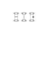
Figure 2: Diagrams contributing to the one-loop renormalization of the mesonic operators.

In Appendix D we compute the one-loop dilatation operator acting on the basis of states ${\cal O}\equiv\bar{Q}_{\cal I}Q^{\cal J}$, evaluating the diagrams schematically drawn in Figure 2. We find

$$\Gamma^{(1)}=\frac{\lambda}{4\pi^{2}}\,\mathbb{K}\,,\quad\mathbb{K}\equiv\delta^{\cal I}_{\cal J}\delta^{\cal K}_{\cal L}\,.$$ (21)

The eigenstates are the triplet and the singlet, with eigenvalues

$$\gamma_{\bf{3}}=0\,,\quad\gamma_{\bf{1}}=\frac{\lambda}{2\pi^{2}}\,.$$ (22)

As expected, the chiral triplet operator has protected dimension. At one-loop, this result does not change as we turn on non-zero angles $\theta_{1}$ and $\theta_{2}$.

So far we have considered the case of a single $D7$ brane, or a single flavor. For multiple $D7$ branes (multiple flavors) the Chan-Paton labels of the open strings are interpreted as the bifundamental flavor indices of the mesonic operators, ${\cal O}^{ij}$, $i,j=1,\dots N_{f}$. In our setup, with $N_{f}=2$, the lowest mode of the open string with off-diagonal Chan-Paton labels, which is the massless gauge field for parallel branes, becomes tachyonic as we turn on a relative angle between the $D7$s. In the dual field theory we expect to find an instability associated with the operator ${\cal O}_{\bf 3}^{12}$, the lowest dimensional operator dual to the off-diagonal open string mode.

3 “Double-trace” Renormalization and the Open String Tachyon

Our setup is an open string version of the phenomena studied in [18, 19, 20, 21]. Motivated by the work of [19, 20], we considered in [21] a generic large $N$, non-supersymmetric field theory with all matter in the adjoint (or bifundamental) representation. We further assumed the theory to be “conformal in its single-trace sector”, by which we mean that all single-trace couplings have vanishing beta function for large $N$. In such a theory, quantum effects induce double-trace couplings of the schematic form

$$\delta S=f\int d^{4}x\,{\cal O}\bar{{\cal O}}\,,\quad{\cal O}\sim\mbox{Tr}\,\phi^{2}\,,$$ (23)

where $\phi$ is a scalar field. The beta function for $f$ may or may not admit a real fixed point. If $\beta_{f}$ has no real zeros, conformal invariance is broken. A closely related phenomenon is the generation of a Coleman-Weinberg potential $\mathcal{V}\left(\langle\phi\rangle\right)$ [18]. It is not difficult to show [21] that the symmetric vacuum $\langle\phi\rangle=0$ is stable if and only if $\beta_{f}$ has a fixed point; conversely, if $\beta_{f}$ has no real zeros, dynamical symmetry breaking occurs.

Field theories of the kind just described arise in several examples of the AdS/CFT correspondence. The best known cases are non-supersymmetric orbifolds of ${\cal N}=4$ SYM, dual to Type IIB string theory on $AdS_{5}\times S^{5}/\Gamma$ with $\Gamma$ a subgroup of $SU(4)_{R}$ (but not a subgroup of $SU(3)$). The field theory instability associated with double-trace renormalization is the boundary counterpart of the instability associated with a closed string tachyon in the AdS bulk. By a tachyon we mean a bulk scalar that violates the Breinlohner-Freedman bound. As usual, the weakly coupled boundary theory (small ’t Hooft coupling $\lambda$) gives information about the high curvature regime of the bulk theory and vice versa. In some examples (non-freely acting orbifolds of ${\cal N}=4$ SYM), the instability is visible both in the weakly curved bulk theory and in the one-loop analysis of the boundary theory; presumably the theory is unstable for all couplings. In other examples (freely acting orbifolds of ${\cal N}=4$) an instability shows up in the one-loop analysis of the boundary theory, but the spectrum of the weakly curved bulk theory has no tachyon; the tachyon must become massive for $\lambda$ greater than some critical value.

We showed in [21] that at large $N$ the conformal dimension $\Delta_{{\cal O}}$ and the beta function $\beta_{f}$ take the general forms

$$\Delta_{{\cal O}}=2+\gamma(\lambda)+\frac{v(\lambda)}{1+\gamma(\lambda)}f\,,$$ (24)

$$\beta_{f}=\frac{v(\lambda)}{1+\gamma(\lambda)}f^{2}+2\gamma(\lambda)f+a(\lambda)\,.$$ (25)

Here $v(\lambda)$ is defined as the normalization coefficient of ${\cal O}$,

$$\langle{\cal O}(x)\bar{\cal O}(0)\rangle=\frac{v(\lambda)}{2\pi^{2}x^{2\Delta(\lambda)}}\,\,;$$ (26)

$\gamma(\lambda)$ is the contribution to the anomalous dimension of ${\cal O}$ from single-trace interactions; finally $a(\lambda)$ is the coefficient of the induced double-trace terms, coming from the single trace interactions, in the quantum effective potential. The expressions (24, 25) are valid to all orders in planar perturbation theory: large $N$ factorization implies that $\beta_{f}$ depends at most quadratically on $f$, and $\Delta_{{\cal O}}$ at most linearly [21] . The coefficients $v(\lambda)$, $\gamma(\lambda)$ and $a(\lambda)$ have planar perturbative expansions

$$v(\lambda)=\sum_{L=1}^{\infty}v^{(L)}\lambda^{L-1}\,,\quad\gamma(\lambda)=\sum_{L=1}^{\infty}\gamma^{(L)}\lambda^{L}\,,\quad a(\lambda)=\sum_{L=1}^{\infty}a^{(L)}\lambda^{L+1}\,,$$ (27)

where the $L$ denotes the loop order. Consider the discriminant of the quadratic equation $\beta_{f}=0$,

$$D(\lambda)\equiv\gamma(\lambda)^{2}-\frac{a(\lambda)\,v(\lambda)}{1+\gamma(\lambda)}\,.$$ (28)

If $D(\lambda)<0$, there are no physical (real) values of $f$ for which the theory is conformal. But if we insist on formally preserving conformal invariance by tuning $f$ to one of its two complex fixed points, then the operator dimension also becomes complex,

$$\Delta_{{\cal O}}=2\pm\,i\,b(\lambda)\,,\qquad b(\lambda)\equiv\sqrt{|D|}\,.$$ (29)

Using the usual AdS/CFT dictionary

$$\Delta_{{\cal O}}=\frac{d}{2}\pm\sqrt{\frac{d^{2}}{4}+m^{2}R^{2}}=2\pm\sqrt{4+m^{2}R^{2}}\,,$$ (30)

we find that the $AdS_{5}$ scalar dual to ${\cal O}$ has mass [21]

$$m^{2}(\lambda)R^{2}=m^{2}_{BF}R^{2}+D(\lambda)=-4+D(\lambda)\,.$$ (31)

For negative discriminant $m^{2}(\lambda)<m^{2}_{BF}$: the scalar field dual to ${\cal O}$ is a true tachyon and the bulk theory is unstable.

We now generalize this story to AdS/CFT dual pairs containing an open string sector. In the presence of flavor branes in the AdS bulk, the dual field theory contains extra fundamental matter. An open string tachyon corresponds to an instability in the mesonic sector of the boundary theory. In this paper we illustrate this phenomenon in the example of the intersecting $D7$ brane system. The classical Lagrangian of the boundary theory takes the schematic form

$${\cal L}={\cal L}_{adjoint}+{\cal L}_{fund}=-\mbox{Tr}\left[F^{2}+\left(DX\right)^{2}+\dots\right]-\left(DQ\right)^{2}-\frac{\lambda}{N}{\cal O}^{ij}{\bar{\cal O}}^{ij}+\dots$$ (32)

where ${\cal O}^{ij}=Q^{i\,\mathfrak{a}}\bar{Q}_{j\,\mathfrak{a}}$ are the gauge-invariant mesonic operators made from the fundamental scalars and for simplicity we have ignored the $SU(2)_{R}$ structure, which will be restored shortly. The whole ${\cal L}_{fund}$ is $1/N$ suppressed with respect to ${\cal L}_{adjoint}$, in harmony with the fact that the classical D-brane effective action arises from worldsheets with disk topology, and is thus suppressed by a power of $g_{s}\sim 1/N$ with respect to the classical closed string effective action, arising from worldsheets with sphere topology. Nevertheless, as always in the tachyon condensation problem, it makes perfect sense to focus on classical open string field theory. The classical open string dynamics is dual to the quantum planar dynamics of the mesonic sector of the field theory. The ’t Hooft coupling $\lambda$ does not run at leading order in $N$, indeed the hyper multiplet contribute to $\beta_{\lambda}$ at order $O(1/N)$. For generic angles, the term in the $Q^{4}$ potential that mix the two flavors run, so perturbative renormalizability forces the introduction of a new coupling constant $f$,

$$\delta{\cal L}_{fund}=-\frac{f}{N}{\cal O}^{12}{\bar{\cal O}}^{12}\,.$$ (33)

Note on the other hand that no extra terms diagonal in flavor (namely ${\cal O}^{11}{\bar{\cal O}}^{11}$ and ${\cal O}^{22}{\bar{\cal O}}^{22}$ are induced at one-loop. For the first flavor this is immediate to see: the diagrams contributing to the term ${\cal O}^{11}{\bar{\cal O}}^{11}$ of the effective potential are independent of $\theta_{1}$, $\theta_{2}$ (they do not involved any coupling mixing the two flavors) and thus their sum must vanish, as it does in the ${\cal N}=2$ supersymmetric theory with $\theta_{1}=\theta_{2}=0$. For the second flavor this follows by symmetry, since the two flavors are of course interchangeable.

This extra “double-trace” term (33) arise at the same order in $N$ order as the classical ${\cal L}_{fund}$, indeed inspection of the Feynman diagrams shows that the one-loop bare coupling $f_{0}$ behaves as

$$f_{0}\sim\lambda^{2}\log\Lambda\,.$$ (34)

The analysis [21] can be applied in its entirety to this “open string” case. The “double-trace” beta function $\beta_{f}$ takes again the form (25), and its discriminant $D(\lambda)$ computes now (through (31) the mass of the open string tachyon dual to mesonic operator ${\cal O}^{12}$. Let us turn to explicit calculations.

3.1 The one-loop “double-trace” beta function

To proceed, we need to be more precise about the structure of the“double-trace” terms induced at one-loop, restoring their $SU(2)_{R}$ structure. For general angles $\theta_{1}$ and $\theta_{2}$, there are three independent structures,

$$\delta{\cal L}_{fund}=-\frac{1}{N}\left[f_{{\bf 3}^{\pm}}\left({\cal O}_{{\bf 3}^{+}}^{12}{\cal O}^{21}_{{\bf 3}^{-}}+{\cal O}_{{\bf 3}^{-}}^{12}{{\cal O}}^{21}_{{\bf 3}^{+}}\right)+f_{{\bf 3}^{0}}{\cal O}_{{\bf 3}^{0}}^{12}{{\cal O}}^{21}_{{\bf 3}^{0}}+f_{{\bf 1}}{\cal O}_{{\bf 1}}^{12}{{\cal O}}^{21}_{{\bf 1}}\right]\,.$$ (35)

We have imposed neutrality under the Cartan of $SU(2)_{R}$, since this is an exact symmetry for generic angles, corresponding geometrically to rotations in the 67 plane (more precisely a 67 rotation is a linear combination of the Cartan of $SU(2)_{L}$ and $SU(2)_{R}$, but the hyper multiplets are neutral under $SU(2)_{L}$). When one of the angles is zero, say $\theta_{2}=0$, rotations in the 567 directions a symmetry (again a diagonal combination of $SU(2)_{L}$ and $SU(2)_{R}$), implying $f_{{\bf 3}^{\pm}}=f_{{\bf 3}^{0}}\equiv f_{\bf 3}$. We focus on the triplet mesons, which are dual to the open string tachyon. For a single non-zero angle there is one beta function $\beta_{f_{{\bf 3}}}$ to compute, since the three components of the triplet are related by symmetry. For generic angles there are in principle two distinct beta functions $\beta_{f_{{\bf 3}^{\pm}}}$ and $\beta_{f_{{\bf 3}^{0}}}$; we will illustrate our method computing the first, which is a slightly simpler calculation. At one-loop, the “double-trace” beta function takes the form

$$\beta_{f}=v^{(1)}f^{2}+2\gamma^{(1)}\lambda f+a^{(1)}\lambda^{2}\,.$$ (36)

We have seen that $\gamma^{(1)}=0$ at one loop for the triplet mesons. The normalization coefficient $v^{(1)}$ is easily evaluated by free Wick contractions,

$$\langle{\cal O}^{12}_{\bf{3}^{0}}\,(x){\cal O}^{21}_{\bf{3}^{0}}\,(y)\rangle=\langle{\cal O}^{12}_{\bf{3}^{+}}\,(x){\cal O}^{21}_{\bf{3}^{-}}\,(y)\rangle=\langle{\cal O}^{12}_{\bf{3}^{-}}\,(x){\cal O}^{21}_{\bf{3}^{+}}\,(y)\rangle=\frac{1}{16\pi^{4}|x-y|^{4}}\,,$$ (37)

implying

$$v_{\bf{3}^{+}}^{(1)}=v_{\bf{3}^{-}}^{(1)}=v_{\bf{3}^{0}}^{(1)}=\frac{1}{8\pi^{2}}\,.$$ (38)

It remains to evaluate the coefficient $a^{(1)}$. We are going to extract $a^{(1)}$ from the one-loop Coleman-Weinberg potential along the “Higgs branch” of the gauge theory, $\langle X_{AB}\rangle=0$, ${\cal Q}^{\cal I}\neq 0$. We put “Higgs branch” in quotes because for general angles it is in fact lifted already at the classical level. Let us first recall the analysis for the ${\cal N}=2$ supersymmetric theory corresponding to two parallel flavor branes are parallel ($\theta_{1}=\theta_{2}=0$).

As always in a supersymmetric theory, flat directions are parametrized by holomorphic gauge-invariant composite operators. In our case the relevant operators are the mesons

$${\cal O}^{ij}=q^{i}\cdot\tilde{q}_{j}\,,\quad i,j=1,2$$ (39)

The dot stands for color contraction $q\cdot{q}^{*}\equiv q^{\mathfrak{a}}\,q^{*}_{\mathfrak{a}}$ and $i,j$ are the flavor indices. The holomorphic, gauge invariant mesons that parameterize the Higgs flat directions are subject to F-flatness conditions

$$q^{\mathfrak{a}\,i}\tilde{q}_{\mathfrak{b}\,i}=0\Leftrightarrow\,{\rm tr}\,{{\cal O}}={\rm det}\,{{\cal O}}=0\,,$$ (40)

thus there are $4-2=2$ complex parameters for the moduli space of the supersymmetric theory ($\theta_{1}=\theta_{2}=0$). We may parameterize the flat directions by

$$Q_{1}=U\left(\begin{array}[]{c}q\\ 0\end{array}\right)\,,\quad Q_{2}=U\left(\begin{array}[]{c}0\\ -q\end{array}\right)\,,\quad U\in SU(2)\quad\mbox{and}\quad q\in\mathbb{R}\,.$$ (41)

Color indices are kept implicit. In color space we may take $q^{\mathfrak{a}=1}=q$ and $q^{\mathfrak{a}\neq 1}=0$. For generic $\theta_{1}$, $\theta_{2}$ supersymmetry is explicitly broken in the classical Lagrangian and the Higgs branch is completely lifted.

To select $\beta_{f_{{\bf 3}^{+}}}$ (which is of course equal to $\beta_{f_{{\bf 3}^{-}}}$), we calculate the effective potential around a classical background such that $\langle{\cal O}_{\bf 1}^{12}\rangle=\langle{\cal O}_{{\bf 3}^{0}}^{12}\rangle=\langle{\cal O}_{{\bf 3}^{-}}^{12}\rangle=0$, but $\langle{\cal O}_{{\bf 3}^{+}}^{12}\rangle\neq 0$, namely

$$Q_{1}=\left(\begin{array}[]{c}q\\ 0\end{array}\right)\,,\quad Q_{2}=\left(\begin{array}[]{c}0\\ -q\end{array}\right)\,,\quad\quad q\in\mathbb{C}$$ (42)

This choice corresponds to the flat direction for the ${\cal N}=1$ susy case $\theta_{1}=\theta_{2}$. The F-terms of the classical potential vanish for general angles, but for $\theta_{1}\neq\theta_{2}$ the D-terms do not, ${\cal V}^{D}_{Q^{4}}=g^{2}|q|^{4}(1-d\left(\theta_{1},\theta_{2}\right))$.

In Appendix E we evaluate the one-loop contribution to the effective potential along this background (at large $N$). With the help of the Callan-Symanzik equation we find

$$a^{(1)}_{{\bf 3}^{\pm}}=\frac{1}{16\pi^{2}}\left[\Big{(}1-d(\theta_{1},\theta_{2})\Big{)}+\frac{1}{2}\Big{(}1-d(\theta_{1},\theta_{2})\Big{)}^{2}+4\,\sin^{2}{\left(\frac{\theta_{1}+\theta_{2}}{2}\right)}\sin^{2}{\left(\frac{\theta_{1}-\theta_{2}}{2}\right)}\,\right]\,.$$ (43)

From our (mild) assumption that the classical potential be positive we have $d(\theta_{1},\theta_{2})\leq 1$, has the crucial implication

$$a^{(1)}_{{\bf 3}^{\pm}}\geq 0\,.$$ (44)

In the supersymmetric case ($\theta_{1}=\theta_{2}$), $a^{(1)}_{{\bf 3}^{\pm}}=0$, as it must. For $\theta_{2}=0$, the $SU(2)$ symmetry is restored, so

$$a^{(1)}_{{\bf 3}^{\pm}}=a^{(1)}_{{\bf 3}^{0}}=\frac{1}{16\pi^{2}}\left[\Big{(}1-d(\theta,0)\Big{)}+\frac{1}{2}\Big{(}1-d(\theta,0)\Big{)}^{2}+4\,\sin^{4}{\left(\frac{\theta}{2}\right)}\,\right]\geq 0\,.$$ (45)

The one-loop triplet beta function (let us focus on the single-angle case)

$$\beta_{f_{\bf 3}}=v^{(1)}_{\bf{3}}\,f^{2}_{\bf 3}+a^{(1)}_{\bf 3}\lambda^{2}$$ (46)

does not admit real fixed points for $f_{\bf 3}$, so conformal invariance is inevitably broken in the quantum theory. The running coupling

$$\bar{f}(\mu)=\frac{a^{(1)}}{\sqrt{v^{(1)}_{\bf{3}}}}\,\lambda^{2}\,\tan\left[\frac{a^{(1)}\lambda^{2}}{\sqrt{v^{(1)}_{\bf{3}}}}\ln(\mu/\mu_{0})\right]$$ (47)

is a monotonically increasing function interpolating between IR and UV Landau poles, at energies

$$\mu_{IR}=\mu_{0}\,\exp\left(-\frac{\pi\sqrt{v^{(1)}_{\bf 3}}}{\lambda\sqrt{a^{(1)}_{\bf{3}}}}\right)\,,\quad\mu_{UV}=\mu_{0}\,\exp\left(\frac{\pi\sqrt{v^{(1)}_{\bf{3}}}}{\lambda\sqrt{a^{(1)}_{\bf{3}}}}\right)\,.$$ (48)

For small coupling $\lambda\to 0$, the Landau poles are pushed respectively to zero and infinity.

3.2 The tachyon mass

As reviewed above, the mass of the field dual to ${\cal O}^{12}_{{\bf 3}^{\pm}}$ is directly related to the discriminant of $\beta_{{\bf 3}^{\pm}}$,

$$m^{2}_{{\bf 3}^{\pm}}R^{2}=m^{2}_{BF}R^{2}+D_{{\bf 3}^{\pm}}(\lambda;\theta_{1},\theta_{2})=-\,4\,-\frac{\lambda^{2}}{16\pi^{4}}\,\mathcal{D}^{(1)}_{\bf{3}}\left(\theta_{1},\theta_{2}\right)+{\cal O}(\lambda^{3})\,,$$ (49)

where

$$\mathcal{D}_{\bf{3}}^{(1)}=\Big{(}1-d(\theta_{1},\theta_{2})\Big{)}+\frac{1}{2}\Big{(}1-d(\theta_{1},\theta_{2})\Big{)}^{2}+4\,\sin^{2}{\left(\frac{\theta_{1}+\theta_{2}}{2}\right)}\sin^{2}{\left(\frac{\theta_{1}-\theta_{2}}{2}\right)}\,.$$ (50)

For $\theta_{1}\neq\theta_{2}$ the discriminant is negative, implying that the bulk field violates the BF stability bound. Whenever supersymmetry is broken, the bulk field dual to ${\cal O}^{12}_{{\bf 3}^{\pm}}$ is a true tachyon. For $\theta_{2}=0$ the $\pm$ and $0$ components of the triplet are related by the $SU(2)$ symmetry and are all tachyonic. We expect the field dual to ${\cal O}^{12}_{{\bf 3}^{0}}$ to be tachyonic for general angles.

For small angles, the $O(\lambda^{2})$ tachyon mass depends on a single unknown parameter $\alpha$ (which enters the parametrization of the classical $Q^{4}$ potential, see Appendix B),

$$R^{2}m_{\bf 3}^{2}(\lambda)=-4-\alpha\,\frac{\lambda^{2}}{16\pi^{4}}\left(\theta_{1}-\theta_{2}\right)^{2}+{\cal O}(\lambda^{3})\,,\qquad\theta_{1}\,,\theta_{2}\ll 1\,.$$ (51)

This expression applies to all three components of the triplet. For the $\pm$ components it is just the expansion of (49) for small angles. For the $0$ component it follows by imposing the symmetry constraints $m_{{\bf 3}^{0}}^{2}(\theta,\theta)=0$ and $m_{{\bf 3}^{0}}^{2}(\theta,0)=m_{{\bf 3}^{\pm}}^{2}(\theta,0)$. By AdS/CFT, we get an interesting prediction for the mass of the open string tachyon for large AdS curvature (small $\lambda$).

Conversely, for large $\lambda$ (small AdS curvature) we can compute the mass of the open string tachyon using the dual string picture. The open string spectrum of branes intersecting at small angles in flat space is well-known. The lowest tachyon mode has mass (see e.g. [27] for a review),

$$m^{2}=-\frac{|\theta_{1}-\theta_{2}|}{\pi^{2}\alpha^{\prime}}\,,,\qquad\theta_{1}\,,\theta_{2}\ll 1\,.$$ (52)

This becomes a good approximation to the mass in the exact AdS sigma model in the limit $\alpha^{\prime}/R^{2}\sim\lambda^{-1/2}\to 0$. Thus

$$\lim_{\lambda\to\infty}R^{2}m_{\bf 3}^{2}(\lambda)=-\frac{|\theta_{1}-\theta_{2}|}{\pi^{2}}\frac{R^{2}}{\alpha^{\prime}}=-\frac{|\theta_{1}-\theta_{2}|}{\pi^{2}}\lambda^{1/2}\,,,\qquad\theta_{1}\,,\theta_{2}\ll 1\,.$$ (53)

This can be regarded as a prediction for the large $\lambda$ behavior of the discriminant $D_{\bf 3}(\lambda)$, which is a purely field-theoretic quantity. Note that apart from the $\lambda$ dependence, which could have been anticipated on general grounds, the weak coupling result (51) and the strong coupling result (53) differ in their angular dependence.

4 Discussion

The main technical question that we leave answered is the precise form of the classical $Q^{4}$ potential for generic angles. As we have emphasized, a superspace formulation of ${\cal N}=4$ SYM with manifest $SU(4)_{R}$ symmetry would offer a solution. It would be interesting to see whether the new off-shell formalism for ${\cal N}=1$ SYM in ten dimensions introduced in [28, 29] could be applied to our problem. In principle, another way to obtain the $Q^{4}$ potential is by taking the decoupling limit of the intersecting brane effective action. This would first require the calculation of a four-point function of twist fields, two twist fields corresponding to D3-D7 open strings and two twist fields corresponding to D3-D7’ open strings. This problem has been solved for branes intersecting at right angles (see e.g. [30, 31, 32, 33]). The generalization to arbitrary angles is an interesting and difficult problem in boundary conformal field theory. Taking the decoupling limit may also be challenging in the presence of tachyons – it is not clear to us whether the result would be unambiguous or it would require some renormalization prescription.

Even without a complete knowledge of the classical $Q^{4}$ potential, by making a plausible positivity assumption we argued that the field theory is unstable at the quantum level. By AdS/CFT, we obtained a non-trivial prediction for the tachyon squared mass $m_{\bf 3}^{2}(\lambda)$ at small $\lambda$. Its behavior at large $\lambda$ is known from flat-space string theory. There must exist an interpolating function $m_{\bf 3}^{2}(\lambda)$ valid for all $\lambda$. It would be extremely interesting to apply integrability techniques to find the whole function. There is a large literature on open spin chains arising in the calculation of anomalous dimensions of mesonic operators, see in particular [34, 35, 36, 37] for our system in the ${\cal N}=2$ supersymmetric case $\theta_{1}=\theta_{2}=0$. It remains to be seen whether the susy-breaking rotation preserves integrability.

Another direction for future work is to study the actual tachyon condensation process on the field theory side. In the bulk, after tachyon condensation the intersecting $D7$ branes recombine (see e.g. [27]). For small $\lambda$, the tachyon vacuum corresponds on the field theory side to the local minimum of the one-loop effective potential. It would be interesting to expand the Lagrangian around the minimum and relate this field theory calculation to the bulk phenomenon of brane recombination.

Appendix A The Supersymmetric Field Theory

In this appendix we spell out our conventions and write the ${\cal N}=2$ supersymmetric action for the usual $D3/D7$ system [2]. We first present the Lagrangian in ${\cal N}=1$ superspace and then in components. Unless otherwise stated, we follow the superspace notations of [24].

As familiar, the ${\cal N}=4$ vector multiplet decomposes into an ${\cal N}=1$ vector multiplet,

$$V=\bar{\theta}\sigma^{\mu}\theta A\,_{\mu}+i\theta^{2}\bar{\theta}\bar{\lambda}-i\bar{\theta}^{2}\theta\lambda+\theta^{2}\bar{\theta}^{2}D\,\quad\mbox{(Wess-Zumino gauge) }$$ (54)

and three chiral multiplets

$$\Phi^{a}=\phi^{a}+\theta\chi^{a}-\theta^{2}F^{a}\,,\quad a=1,2,3\,,$$ (55)

all in the adjoint representation of the $SU(N)$ gauge group. For zero theta angle, the superspace Lagrangian reads

$${\cal L}_{{\cal N}=4}=\mbox{Tr}\left[\int d^{4}\theta\,e^{-gV}\,\bar{\Phi}_{a}\,e^{gV}\,\Phi^{a}+\int d^{2}\theta\,W^{2}+\left(\frac{i\,g}{3!}\int d^{2}\theta\,\epsilon_{abc}\,\Phi^{a}\left[\Phi^{b},\,\Phi^{c}\right]+h.c.\right)\right]\,,$$ (56)

where $W_{\alpha}\equiv i\bar{D}^{2}D_{\alpha}V$ is the usual field strength chiral superfield. In this ${\cal N}=1$ language, only an $SU(3)_{R}\times U(1)_{r}$ subgroup of the $SU(4)_{R}$ $R$-symmetry is visible. The $SU(3)_{R}$ rotates the three chiral superfields leaving $V$ invariant, while the $U(1)_{r}$ is the usual ${\cal N}=1$ $R$-symmetry, with the chiral superfields having charge $2/3$.

In components,

$${\cal L}_{\mathcal{N}=4}=\mbox{Tr}\Bigg{[}-\frac{1}{4}F^{\mu\nu}F_{\mu\nu}-i\bar{\lambda}_{A}\bar{\sigma}^{\mu}D_{\mu}\lambda^{A}-\frac{1}{2}D^{\mu}\bar{X}_{AB}D_{\mu}X^{AB}\Bigg{.}$$

$$\Bigg{.}+i\,\sqrt{2}\,g\,X^{AB}\,\bar{\lambda}_{A}\bar{\lambda}_{B}-i\,\sqrt{2}\,g\,\bar{X}_{AB}\lambda^{A}\lambda^{B}-\frac{g^{2}}{4}[X^{AB},X^{CD}]\,[\bar{X}_{CD},\bar{X}_{AB}]\Bigg{]}\,,$$ (57)

where $A,B=1,\dots,4$. The scalars $X^{AB}$ are related to the three complex scalars $\phi^{a}$ as

$$X^{AB}=\left(\begin{array}[]{cc|cc}0&\phi^{3}&\phi^{2}&\phi^{1}\\ -\phi^{3}&0&\phi^{*}_{1}&-\phi^{*}_{2}\\ \hline\cr-\phi^{2}&-\phi^{*}_{1}&0&\phi^{*}_{3}\\ -\phi^{1}&\phi^{*}_{2}&-\phi^{*}_{3}&0\end{array}\right)$$ (58)

and obey the self-duality constraint (1).

We can also think the ${\cal N}=4$ vector multiplet as an ${\cal N}=2$ vector multiplet (comprising $V$ and $\Phi^{3}$) and an ${\cal N}=2$ hyper multiplet (comprising $\Phi^{1}$ and $\Phi^{2}$). We wish to couple the ${\cal N}=2$ vector multiplet $(V,\Phi^{3})$ to $N_{f}$ “flavor” hyper multiplets in the fundamental representation of the gauge group. Each ${\cal N}=2$ flavor hyper multiplet decomposes into two ${\cal N}=1$ chiral multiplets

$$Q=q+\theta\psi-\theta^{2}f\quad\mbox{and}\quad\tilde{Q}=\tilde{q}+\theta\tilde{\psi}-\theta^{2}\tilde{f}\,,$$

where $Q$ is in the fundamental representation of $SU(N)$ and $\tilde{Q}$ in the antifundamental representation. In ${\cal N}=1$ superspace, the flavor part of the Lagrangian reads

$${\cal L}_{hyper}=\int d^{4}\theta\,\bar{Q}_{i}\,e^{gV}\,Q^{i}+\int d^{4}\theta\,\tilde{Q}_{i}\,e^{-gV}\,\bar{\tilde{Q}}^{i}+\left(g\int d^{2}\theta\,\tilde{Q}_{i}\,\Phi^{3}\,Q^{i}+h.c.\right)\,,$$ (59)

where $i=1,\dots,N_{f}$ is a flavor index. In components,

$${\cal L}_{hyper}=-D^{\mu}\bar{Q}_{{\cal I}\,i}D_{\mu}Q^{{\cal I}\,i}-i\bar{\psi}_{i}\bar{\sigma}^{\mu}D_{\mu}\psi^{i}-i\tilde{\psi}_{i}\sigma^{\mu}D_{\mu}\bar{\tilde{\psi}}\,^{i}$$

$$\left.-\sqrt{2}\,i\,g\,\tilde{\psi}_{i}X^{12}\psi^{i}+\sqrt{2}\,i\,g\,\bar{\psi}_{i}\bar{X}_{12}\bar{\tilde{\psi}}\,^{i}\right.$$

$$\left.+ig\sqrt{2}\bar{Q}_{{\cal I}\,i}\bar{\Lambda}^{{\cal I}}\bar{\tilde{\psi}}\,^{i}-ig\sqrt{2}\tilde{\psi}_{i}\Lambda_{{\cal I}}Q^{{\cal I}\,i}+ig\sqrt{2}\bar{Q}_{{\cal I}\,i}\epsilon^{{\cal I}{\cal J}}\Lambda_{{\cal J}}\psi^{i}-ig\sqrt{2}\bar{\psi}_{i}\bar{\Lambda}^{{\cal I}}\epsilon_{{\cal I}{\cal J}}Q^{{\cal J}\,i}\right.$$

$$-\frac{1}{2}g^{2}\bar{Q}_{{\cal I}\,i}\bar{X}_{AB}X^{AB}Q^{{\cal I}\,i}-g^{2}\bar{Q}_{{\cal J}\,i}\mathcal{X}_{{\cal I}\hat{\cal K}}\mathcal{X}^{{\cal J}\hat{\cal K}}Q^{{\cal I}\,i}\,.$$

$$-\frac{g^{2}}{2}(\bar{Q}_{{\cal I}\,i}\cdot Q^{{\cal J}\,j})(\bar{Q}_{{\cal J}\,j}\cdot Q^{{\cal I}\,i})-g^{2}\epsilon_{{\cal I}{\cal K}}\epsilon^{{\cal L}{\cal J}}(\bar{Q}_{{\cal L}\,i}\cdot Q^{{\cal K}\,j})(\bar{Q}_{{\cal J}\,j}\cdot Q^{{\cal I}\,i})\,.$$ (60)

Following [34], we have introduced the $SU(2)_{R}$ doublets

$$Q^{{\cal I}}\equiv\left(\begin{array}[]{c}q\\ \tilde{q}^{*}\end{array}\right)\,,\quad\Lambda_{{\cal I}}\equiv\left(\begin{array}[]{c}\lambda_{1}\\ \lambda_{2}\end{array}\right)=\left(\begin{array}[]{c}\lambda\\ -\chi_{3}\end{array}\right)\,,\quad{\cal I}=1,2\,.$$ (61)

The other two Weyl spinors can be assembled into an $SU(2)_{L}$ doublet,

$$\hat{\Lambda}_{\hat{\cal I}}\equiv\left(\begin{array}[]{c}\lambda_{3}\\ \lambda_{4}\end{array}\right)=\left(\begin{array}[]{c}-\chi_{2}\\ -\chi_{1}\end{array}\right)\,,$$ (62)

which does not couple to the flavor hyper multiplets. Note that to avoid cluttering we keep color indices implicit. Color contractions are almost always obvious. When ambiguity may arise, we indicate the contraction with a dot. For example in the term

$$(\bar{Q}_{{\cal I}\,i}\cdot Q^{{\cal J}\,j})(\bar{Q}_{{\cal J}\,j}\cdot Q^{{\cal I}\,i})$$ (63)

the first pair is color contracted, and so is the second pair.

The $Q^{4}$ term in the Lagrangian can be written more compactly by introducing flavor-contracted composite operators, in the adjoint of the gauge group,

$${\cal M}_{{\cal J}\,\,\,\mathfrak{b}}^{\,\,{\cal I}\mathfrak{a}}\equiv\frac{1}{\sqrt{2}}Q_{{\cal J}\mbox{ }i}^{\mbox{ }\mathfrak{a}}\,\bar{Q}_{\mbox{ }\mathfrak{b}}^{{\cal I}\mbox{ }i}\,,$$ (64)

which may be decomposed into the $SU(2)_{R}$ singlet and triplet combinations

$${\cal M}_{{\bf{1}}}\equiv{\cal M}^{\,\,{\cal I}}_{{\cal I}}\quad\mbox{and}\quad{\cal M}_{{\bf{3}}{\cal J}}^{\quad{\cal I}}\equiv{\cal M}^{\,\,{\cal I}}_{{\cal J}}-\frac{1}{2}{\cal M}^{\,\,{\cal K}}_{{\cal K}}\,\delta^{{\cal I}}_{{\cal J}}\,.$$ (65)

In terms of the component fields $q$ and $\tilde{q}$,

$${\cal M}_{\bf{1}}=\frac{1}{\sqrt{2}}\left(q\,\bar{q}+\bar{\tilde{q}}\,\tilde{q}\right)$$ (66)

$${\cal M}_{\bf{3}^{+}}=q\,\tilde{q}$$

$${\cal M}_{\bf{3}^{0}}=\frac{1}{\sqrt{2}}\left(q\,\bar{q}-\bar{\tilde{q}}\,\tilde{q}\right)$$

$${\cal M}_{\bf{3}^{-}}=\tilde{q}^{*}\,q^{*}\,,$$

where the superscripts refer to the eigenvalues under the Cartan generator of $SU(2)_{R}$. The $F$ and $\bar{F}$ auxiliary fields couple to ${\cal M}_{{\bf 3}^{\pm}}$, while the $D$ auxiliary field couples to ${\cal M}_{{\bf 3}^{0}}$. Thus the $Q^{4}$ scalar potential is the square of the triplet composite,

$${\cal L}_{Q^{4}}=-g^{2}\,{\rm Tr}\,{\cal M}_{\bf 3}\,{\cal M}_{\bf 3}\equiv-g^{2}\,{\rm Tr}\left[2{\cal M}_{{\bf 3}^{+}}{\cal M}_{{\bf 3}^{-}}+{\cal M}_{{\bf 3}^{0}}{\cal M}_{{\bf 3}^{0}}\right]\,.$$ (67)

Finally, let us write the $Q^{4}$ potential using the gauge-invariant mesonic operators. The explicit expressions of the mesons in components are

$${\cal O}^{ij}_{\bf{1}}=\frac{1}{\sqrt{2}}\left(q^{i\,\mathfrak{a}}\,\bar{q}_{j\,\mathfrak{a}}+\bar{\tilde{q}}^{i\,\mathfrak{a}}\,\tilde{q}_{j\,\mathfrak{a}}\right)$$ (68)

$${\cal O}^{ij}_{\bf{3}^{+}}=q^{i\,\mathfrak{a}}\,\tilde{q}_{j\,\mathfrak{a}}$$

$${\cal O}^{ij}_{\bf{3}^{0}}=\frac{1}{\sqrt{2}}\left(q^{i\,\mathfrak{a}}\,\bar{q}_{j\,\mathfrak{a}}-\bar{\tilde{q}}^{i\,\mathfrak{a}}\,\tilde{q}_{j\,\mathfrak{a}}\right)$$

$${\cal O}^{ij}_{\bf{3}^{-}}=\tilde{q}^{*}\,{}^{i\,\mathfrak{a}}\,q^{*}_{j\,\mathfrak{a}}\,.$$

Withe these definitions,

$${\cal L}_{Q^{4}}=-\frac{g^{2}}{2}\,{\rm Tr}\left(3\,{\cal O}_{\bf 1}^{ij}\,{\cal O}_{\bf 1}^{ij}-{\cal O}_{\bf 3}^{ij}\,{\cal O}_{\bf 3}^{ij}\right)\,.$$ (69)

Appendix B The Field Theory for General Angles

In this appendix we derive the Lagrangian dual to the system with two flavor branes at general angles, up to an ambiguity in the $Q^{4}$ terms of the scalar potential, for which we give a general parametrization. As explained in the text, we need to rotate the ${\cal N}=4$ fields (including in principle the auxiliary fields) in the terms of the Lagrangian where they are coupled to the second hyper multiplet.

B.1 R-symmetry rotations of the ${\cal N}=4$ fields

Rotation of the $X_{m}$ scalars in the 49 plane (with angle $\theta_{1}$) and in the 85 plane (with angle $\theta_{2}$) is performed by the matrix

$${\cal R}^{({\bf 6})}(\theta_{1},\theta_{2})=\left(\begin{array}[]{cccccc}\cos{\theta_{1}}&0&0&\,0&0&-\,\sin{\theta_{1}}\\ 0&\cos{\theta_{2}}&0&\,0&\sin{\theta_{2}}&0\\ 0&0&1&\,0&0&0\\ 0&0&0&\,1&0&0\\ 0&-\,\sin{\theta_{2}}&0&\,0&\cos{\theta_{2}}&0\\ \sin{\theta_{1}}&0&0&\,0&0&\cos{\theta_{1}}\end{array}\right)$$ (70)

A short calculation using the the Clebsh-Gordon coefficients (2) gives the corresponding $SU(4)_{R}$ transformation for the fermions $\lambda_{A}$,

$${\cal R}^{({\bf 4})}(\theta_{1},\theta_{2})=\left(\begin{array}[]{cccc}\cos{\left(\frac{\theta_{1}-\theta_{2}}{2}\right)}&0&i\sin{\left(\frac{\theta_{1}-\theta_{2}}{2}\right)}&0\\ 0&\cos{\left(\frac{\theta_{1}+\theta_{2}}{2}\right)}&0&i\sin{\left(\frac{\theta_{1}+\theta_{2}}{2}\right)}\\ i\sin{\left(\frac{\theta_{1}-\theta_{2}}{2}\right)}&0&\cos{\left(\frac{\theta_{1}-\theta_{2}}{2}\right)}&0\\ 0&i\sin{\left(\frac{\theta_{1}+\theta_{2}}{2}\right)}&0&\cos{\left(\frac{\theta_{1}+\theta_{2}}{2}\right)}\end{array}\right)\,.$$ (74)

Ideally, at this point we would provide the corresponding $SU(4)_{R}$ transformation of the $F$ and $D$ auxiliary fields. An unsuccessful attempt to find such transformation rules using the formalism of [23, 24] is described in Appendix C.

Clearly, the ${\cal N}=4$ part does not depend on the angles, since $SU(4)_{R}$ is an exact symmetry,

$${\cal L}_{total}(\theta)={\cal L}_{{\cal N}=4}+{\cal L}_{hyper}(\theta)\,.$$ (75)

We write

$${\cal L}_{hyper}(\theta)={\cal L}_{kin}+{\cal L}^{(1)}_{Yukawa}+{\cal L}^{(1)}_{\bar{Q}X^{2}Q}+{\cal L}^{(2)}_{Yukawa}(\theta)+{\cal L}^{(2)}_{\bar{Q}X^{2}Q}(\theta)+{\cal L}_{Q^{4}}(\theta)\,,$$ (76)

where the superscripts $(1)$ and $(2)$ refer to the first and second flavor, respectively. We have indicated which terms are $\theta$ dependent. The terms ${\cal L}^{(2)}_{Yukawa}(\theta)$ and ${\cal L}^{(2)}_{\bar{Q}X^{2}Q}(\theta)$ are fixed unambiguously by the transformations (70, 74). By contrast to determine ${\cal L}_{Q^{4}}(\theta)$ we would need an off-shell superspace formulation for the ${\cal N}=4$ multiplet, which is not available at present.

The terms that we can fix are:

$${\cal L}_{kin}=-D^{\mu}\bar{q}_{i}D_{\mu}q^{i}-D^{\mu}\tilde{q}_{i}D_{\mu}\bar{\tilde{q}}^{i}-i\bar{\psi}_{i}\bar{\sigma}^{\mu}D_{\mu}\psi^{i}-i\tilde{\psi}_{i}\sigma^{\mu}D_{\mu}\bar{\tilde{\psi}}\,^{i}$$ (77)

$${\cal L}^{(1)}_{Yukawa}= -\sqrt{2}ig\,\tilde{\psi}_{1}\,\lambda_{1}\,q^{1}-\sqrt{2}ig\,\tilde{q}_{1}\,\lambda_{1}\,\psi^{1}-\sqrt{2}ig\,\bar{\psi}_{1}\,\bar{\lambda}^{2}\,q^{1}-\sqrt{2}ig\,\tilde{\psi}_{1}\,\lambda_{2}\,\tilde{q}^{*}\,{}^{1}$$ (78)

$$-i\,g\,\tilde{\psi}_{1}\left(X_{8}+iX_{9}\right)\psi^{1}\,+\,h.c.$$

$${\cal L}^{(1)}_{\bar{Q}X^{2}Q} = -i\,g^{2}\,\,q^{*}_{1}\,\Big{(}\left[\,X_{4}\,,\,X_{6}\,\right]+i\left[\,X_{4}\,,\,X_{7}\,\right]+i\left[\,X_{5}\,,\,X_{6}\,\right]-\left[\,X_{5}\,,\,X_{7}\,\right]\Big{)}\,\tilde{q}^{*}\,{}^{1}$$

$$-i\,g^{2}\,\tilde{q}_{1}\,\Big{(}\left[\,X_{4}\,,\,X_{6}\,\right]-i\left[\,X_{4}\,,\,X_{7}\,\right]-i\left[\,X_{5}\,,\,X_{6}\,\right]-\left[\,X_{5}\,,\,X_{7}\,\right]\Big{)}\,q^{1}$$

$$+\,i\,g^{2}\,q^{*}_{1}\,\Big{(}\left[\,X_{4}\,,\,X_{5}\,\right]+\,\left[\,X_{6}\,,\,X_{7}\,\right]\Big{)}\,q^{1}$$

$$-\,i\,g^{2}\,\tilde{q}_{1}\,\Big{(}\left[\,X_{4}\,,\,X_{5}\,\right]+\,\left[\,X_{6}\,,\,X_{7}\,\right]\Big{)}\,\tilde{q}^{*}\,{}^{1}$$

$$-\,g^{2}\,q^{*}_{1}\,\Big{(}X_{8}^{2}+X_{9}^{2}\Big{)}\,q^{1}-\,g^{2}\,\tilde{q}_{1}\,\Big{(}X_{8}^{2}+X_{9}^{2}\Big{)}\,\tilde{q}^{*}\,{}^{1}$$

$${\cal L}^{(2)}_{Yukawa}(\theta) = -\sqrt{2}ig\,\cos{\left(\frac{\theta_{1}-\theta_{2}}{2}\right)}\,\tilde{\psi}_{2}\,\lambda_{1}\,q^{2}+\sqrt{2}g\,\sin{\left(\frac{\theta_{1}-\theta_{2}}{2}\right)}\,\tilde{\psi}_{2}\,\lambda_{3}\,q^{2}$$

$$- \sqrt{2}ig\,\tilde{q}_{2}\,\cos{\left(\frac{\theta_{1}-\theta_{2}}{2}\right)}\,\lambda_{1}\,\psi^{2}+\sqrt{2}g\,\tilde{q}_{2}\,\sin{\left(\frac{\theta_{1}-\theta_{2}}{2}\right)}\,\lambda_{3}\,\psi^{2}$$

$$- \sqrt{2}ig\,\cos{\left(\frac{\theta_{1}+\theta_{2}}{2}\right)}\,\bar{\psi}_{2}\,\bar{\lambda}^{2}\,q^{2}-\sqrt{2}g\,\sin{\left(\frac{\theta_{1}+\theta_{2}}{2}\right)}\,\bar{\psi}_{2}\,\bar{\lambda}^{4}\,q^{2}$$

$$- \sqrt{2}ig\,\cos{\left(\frac{\theta_{1}+\theta_{2}}{2}\right)}\,\tilde{\psi}_{2}\,\lambda_{2}\,\tilde{q}^{*}\,{}^{2}+\sqrt{2}g\,\sin{\left(\frac{\theta_{1}+\theta_{2}}{2}\right)}\,\tilde{\psi}_{2}\,\lambda_{4}\,\tilde{q}^{*}\,{}^{2}$$

$$- i\,g\,\tilde{\psi}_{2}\left(\cos{\theta_{2}}\,X_{8}+\sin{\theta_{2}}X_{5}+i\cos{\theta_{1}}\,X_{9}-i\sin{\theta_{1}}X_{4}\right)\psi^{2}+h.c.$$

$${\cal L}^{(2)}_{\bar{Q}X^{2}Q}(\theta) = -\,i\,g^{2}\,q^{*}_{2}\,\Big{(}\cos{\theta_{1}}\left(\left[\,X_{4}\,,\,X_{6}\,\right]+i\left[\,X_{4}\,,\,X_{7}\,\right]\right)+\cos{\theta_{2}}\left(i\left[\,X_{5}\,,\,X_{6}\,\right]-\left[\,X_{5}\,,\,X_{7}\,\right]\right)\Big{)}\,\tilde{q}^{*}\,{}^{2}$$

$$-\,i\,g^{2}\,\tilde{q}_{2}\,\Big{(}\cos{\theta_{1}}\left(\left[\,X_{4}\,,\,X_{6}\,\right]-i\left[\,X_{4}\,,\,X_{7}\,\right]\right)+\cos{\theta_{2}}\left(-i\left[\,X_{5}\,,\,X_{6}\,\right]-\left[\,X_{5}\,,\,X_{7}\,\right]\right)\Big{)}\,q^{2}$$

$$-\,i\,g^{2}\,q^{*}_{2}\,\Big{(}-\sin{\theta_{1}}\left(\left[\,X_{9}\,,\,X_{6}\,\right]+i\left[\,X_{9}\,,\,X_{7}\,\right]\right)+\sin{\theta_{2}}\left(i\left[\,X_{8}\,,\,X_{6}\,\right]-\left[\,X_{8}\,,\,X_{7}\,\right]\right)\Big{)}\,\tilde{q}^{*}\,{}^{2}$$

$$-\,i\,g^{2}\,\tilde{q}_{2}\,\Big{(}-\sin{\theta_{1}}\left(\left[\,X_{9}\,,\,X_{6}\,\right]-i\left[\,X_{9}\,,\,X_{7}\,\right]\right)+\sin{\theta_{2}}\left(-i\left[\,X_{8}\,,\,X_{6}\,\right]-\left[\,X_{8}\,,\,X_{7}\,\right]\right)\Big{)}\,q^{2}$$

$$+\,i\,g^{2}\,q^{*}_{2}\,\Big{(}\cos{\theta_{1}}\cos{\theta_{2}}\left[\,X_{4}\,,\,X_{5}\,\right]+\,\left[\,X_{6}\,,\,X_{7}\,\right]-\sin{\theta_{1}}\sin{\theta_{2}}\,\left[\,X_{8}\,,\,X_{9}\,\right]\Big{)}\,q^{2}$$

$$+\,i\,g^{2}\,q^{*}_{2}\,\Big{(}\cos{\theta_{1}}\sin{\theta_{2}}\left[\,X_{4}\,,\,X_{8}\,\right]-\sin{\theta_{1}}\cos{\theta_{2}}\,\left[\,X_{5}\,,\,X_{9}\,\right]\Big{)}\,q^{2}$$

$$-\,i\,g^{2}\,\tilde{q}_{2}\,\Big{(}\cos{\theta_{1}}\cos{\theta_{2}}\left[\,X_{4}\,,\,X_{5}\,\right]+\,\left[\,X_{6}\,,\,X_{7}\,\right]-\sin{\theta_{1}}\sin{\theta_{2}}\,\left[\,X_{8}\,,\,X_{9}\,\right]\Big{)}\,\tilde{q}^{*}\,{}^{2}$$

$$-\,i\,g^{2}\,\tilde{q}_{2}\,\Big{(}\cos{\theta_{1}}\sin{\theta_{2}}\left[\,X_{4}\,,\,X_{8}\,\right]-\sin{\theta_{1}}\cos{\theta_{2}}\,\left[\,X_{5}\,,\,X_{9}\,\right]\Big{)}\,\tilde{q}^{*}\,{}^{2}$$

$$-\,g^{2}\,q^{*}_{2}\left(\,\Big{|}\cos{\theta_{2}}\,X_{8}+\sin{\theta_{2}}X_{5}\Big{|}^{2}+\Big{|}\cos{\theta_{1}}\,X_{9}-\sin{\theta_{1}}X_{4}\Big{|}^{2}\right)\,q^{2}$$

$$-\,g^{2}\,\tilde{q}_{2}\left(\,\Big{|}\cos{\theta_{2}}\,X_{8}+\sin{\theta_{2}}X_{5}\Big{|}^{2}+\Big{|}\left(\cos{\theta_{1}}\,X_{9}-\sin{\theta_{1}}X_{4}\right)\Big{|}^{2}\right)\,\tilde{q}^{*}\,{}^{2}\,\,.$$

B.2 Parametrizing the $Q^{4}$ potential

Writing

$$-{\cal L}_{Q^{4}}(\theta_{1},\theta_{2})=V_{Q_{1}^{4}}+V_{Q_{2}^{4}}+V_{Q_{1}^{2}Q_{2}^{2}}(\theta_{1},\theta_{2})\,,$$ (81)

it is clear that the terms $V_{Q_{1}^{4}}$ and $V_{Q_{2}^{4}}$ (involving respectively only the scalars of the first and second hyper multiplet) are unaffected by the rotation. Indeed if we set to zero one of the two hyper multiplets we must recover the standard supersymmetric Lagrangian (possibly after a change of variables: if we set to zero the first hyper multiplet in (76) we must rotate back the $X$ and $\lambda$ fields to restore $\bar{Q}X^{2}Q$ and Yukawa terms to the standard form).

Recall (Appendix A) that the potential for a single flavor $Q_{1}$ is

$$V_{Q_{1}^{4}}={\rm Tr}\,\left[2\,{\cal M}^{11}_{{\bf 3}^{+}}{\cal M}^{11}_{{\bf 3}^{-}}+{\cal M}^{11}_{{\bf 3}^{0}}{\cal M}^{11}_{{\bf 3}^{0}}\right]\,,$$ (82)

where ${\cal M}_{\bf 3}^{11}\sim(Q_{i=1}\bar{Q}^{i=1})_{\bf 3}$ is the color–adjoint composite in the triplet of $SU(2)_{R}$ containing only scalars in the first flavor $i=1$ (compare with (65)), and similarly of course for $V_{Q_{2}^{4}}$, with ${\cal M}_{\bf 3}^{11}\to{\cal M}_{\bf 3}^{22}\sim(Q_{i=2}\bar{Q}^{i=2})_{\bf 3}$. The mixed terms can be parametrized by two unknown functions of the angles,

$$V_{Q_{1}^{2}Q_{2}^{2}}=2\,g^{2}\,{\rm Tr}\,\Big{[}f\left(\theta_{1},\theta_{2}\right)\left({\cal M}^{11}_{{\bf 3}^{+}}{\cal M}^{22}_{{\bf 3}^{-}}+{\cal M}^{11}_{{\bf 3}^{-}}{\cal M}^{22}_{{\bf 3}^{+}}\right)+d\left(\theta_{1},\theta_{2}\right)\,{\cal M}^{11}_{{\bf 3}^{0}}{\cal M}^{22}_{{\bf 3}^{0}}\Big{]}\,.$$ (83)

We have imposed neutrality of the potential under a Cartan generator $U(1)\subset SU(2)_{R}$. This $U(1)$ is preserved for general $\theta_{1}$, $\theta_{2}$ and corresponds geometrically to rotations in the 67 plane. When one of the two angles is zero, say $\theta_{2}=0$, an $SU(2)$ symmetry is preserved, corresponding geometrically to rotations in the 567 directions, which is a certain diagonal combination of $SU(2)_{L}$ and $SU(2)_{R}$. The hyper multiplets are neutral under $SU(2)_{L}$, so under a 567 rotation they just undergo just an $SU(2)_{R}$. It follows that for $\theta_{2}=0$ the $Q^{4}$ must be $SU(2)_{R}$ invariant and the functions $f$ and $d$ are related as

$$f\left(\theta,0\right)=d\left(\theta,0\right)\,.$$ (84)

The only assumption we have made in writing (83) is that the rotation does not introduce any terms containing the $SU(2)_{R}$ singlet composites ${\cal M}_{\bf 1}^{11}$ and ${\cal M}_{\bf 1}^{22}$. This is generally the case if the rotated Lagrangian can be obtained from some off-shell superspace formulation of ${\cal N}=4$ SYM with manifest $SU(4)_{R}$ symmetry. Indeed we know that for zero angles the ${\cal N}=4$ auxiliary fields only couple to ${\cal M}_{\bf 3}$, and rotating the auxiliary fields can never generate ${\cal M}_{\bf 1}$.

When $\theta_{1}=\theta_{2}=\theta$ ${\cal N}=1$ supersymmetry is preserved, and the $SU(4)$ $R$-symmetry transformation corresponds to a matrix ${\cal R}^{({\bf 4})}\subset SU(3)$, which acts on $F^{a}$ leaving $D$ invariant. This is a manifest symmetry of the ${\cal N}=1$ superspace formulation. As reviewed in Appendix C, in this special case one can unambiguously find

$$f\left(\theta,\theta\right)=\cos{\theta}$$ (85)

$$d\left(\theta,\theta\right)=1\,.$$

Further constraints follow from discrete symmetries. The 89 reflection $X_{8},X_{9}\rightarrow-X_{8},-X_{9}$ corresponds

$$\theta_{1}\,,\theta_{2}\rightarrow-\theta_{1}\,,-\theta_{2}\,.$$ (86)

Invariance of the $Q^{4}$ potential under this parity symmetry implies

$$f\left(\theta_{1},\theta_{2}\right)=f\left(-\theta_{1},-\theta_{2}\right)$$ (87)

$$d\left(\theta_{1},\theta_{2}\right)=d\left(-\theta_{1},-\theta_{2}\right)\,.$$ (88)

Similarly, invariance under the discrete symmetry $X_{4}\leftrightarrow X_{5}$ and $X_{8}\leftrightarrow X_{9}$, or

$$\theta_{1}\leftrightarrow\theta_{2}\,,$$ (89)

implies

$$f\left(\theta_{1},\theta_{2}\right)=f\left(\theta_{2},\theta_{1}\right)\quad\mbox{and}\quad d\left(\theta_{1},\theta_{2}\right)=d\left(\theta_{2},\theta_{1}\right)\,.$$ (90)

Unfortunately this set of relations is not sufficient to fix the functions $f$ and $d$ uniquely.

A crucial assumption we shall make is positivity of the classical $Q^{4}$ potential. It would follow from the existence of a superspace formulation with manifest $SU(4)_{R}$ symmetry: the scalar potential would be proportional to the square of some auxiliary fields, and it would thus be positive even the susy-breaking $SU(4)_{R}$ rotation in the terms that couple the auxiliary fields to the second hyper multiplet. Assuming positivity, we have

$$V_{Q^{4}}\geq 0\quad\Rightarrow\quad f\left(\theta_{1},\theta_{2}\right)\leq 1\quad\mbox{and}\quad d\left(\theta_{1},\theta_{2}\right)\leq 1\quad\forall\,\theta_{1},\theta_{2}\,.$$ (91)

For small angles, taking into account the discrete symmetries, we can expand

$$f\left(\theta_{1},\theta_{2}\right) = 1-\alpha(\theta_{1}^{2}+\theta_{2}^{2})-\beta\theta_{1}\theta_{2}+O(\theta^{3})$$ (92)

$$d\left(\theta_{1},\theta_{2}\right) = 1-\tilde{\alpha}\left(\theta_{1}^{2}+\theta_{2}^{2}\right)-\tilde{\beta}\theta_{1}\theta_{2}+O(\theta^{3})$$ (93)

for some coefficients $\alpha,\beta,\tilde{\alpha},\tilde{\beta}$. Imposing (85) gives $2\alpha+\beta=\frac{1}{2}$ and $2\tilde{\alpha}+\tilde{\beta}=0$, while (84) gives $\alpha=\tilde{\alpha}$. This leaves us with with a single unknown coefficient,

$$f\left(\theta_{1},\theta_{2}\right) = 1-\alpha(\theta_{1}-\theta_{2})^{2}-\frac{1}{2}\theta_{1}\theta_{2}+O(\theta^{3})$$ (94)

$$d\left(\theta_{1},\theta_{2}\right) = 1-\alpha\left(\theta_{1}-\theta_{2}\right)^{2}+O(\theta^{3})\,.$$ (95)

Positivity of the $Q^{4}$ potential implies that $\alpha>0$.

Finally we record the explicit expressions of the $Q^{4}$ terms, both in terms of component fields,

$${\cal L}_{Q^{4}}(\theta_{1},\theta_{2}) = -2\,g^{2}\left(\tilde{q}_{1}\cdot\tilde{q}^{*}\,{}^{1}\right)\left(q^{*}_{1}\cdot q^{1}\right)-2\,g^{2}\left(\tilde{q}_{2}\cdot\tilde{q}^{*}\,{}^{2}\right)\left(q^{*}_{2}\cdot q^{2}\right)$$

$$-2\,g^{2}f\left(\theta_{1},\theta_{2}\right)\,\Big{[}\left(\tilde{q}_{1}\cdot\tilde{q}^{*}\,{}^{2}\right)\left(q^{*}_{2}\cdot q^{1}\right)+\left(\tilde{q}_{2}\cdot\tilde{q}^{*}\,{}^{1}\right)\left(q^{*}_{1}\cdot q^{2}\right)\Big{]}$$

$$-\frac{g^{2}}{2}\,\left(q^{1}\,q^{*}_{1}-\tilde{q}^{*}\,{}^{1}\,\tilde{q}_{1}\right)^{2}-\frac{g^{2}}{2}\left(q^{2}\,q^{*}_{2}-\tilde{q}^{*}\,{}^{2}\,\tilde{q}_{2}\right)^{2}$$

$$-g^{2}d\left(\theta_{1},\theta_{2}\right)\left(q^{1}\,q^{*}_{1}-\tilde{q}^{*}\,{}^{1}\,\tilde{q}_{1}\right)\cdot\left(q^{2}\,q^{*}_{2}-\tilde{q}^{*}\,{}^{2}\,\tilde{q}_{2}\right)\,,$$

and in terms of the gauge invariant mesonic operators,

$${\cal L}_{Q^{4}}(\theta_{1},\theta_{2}) = -\frac{g^{2}}{2}\,{\rm Tr}\Big{[}3\,{\cal O}_{\bf 1}^{11}\,{\cal O}_{\bf 1}^{11}-{\cal O}_{\bf 3}^{11}\,{\cal O}_{\bf 3}^{11}\Big{]}-\frac{g^{2}}{2}\,{\rm Tr}\Big{[}3\,{\cal O}_{\bf 1}^{22}\,{\cal O}_{\bf 1}^{22}-{\cal O}_{\bf 3}^{22}\,{\cal O}_{\bf 3}^{22}\Big{]}$$ (98)

$$-\,g^{2}\left(d\left(\theta_{1},\theta_{2}\right)+2\,f\left(\theta_{1},\theta_{2}\right)\right)\,{\rm Tr}\Big{[}{\cal O}_{\bf 1}^{12}\,{\cal O}_{\bf 1}^{21}\Big{]}$$

$$-\,g^{2}\left(d\left(\theta_{1},\theta_{2}\right)-2\,f\left(\theta_{1},\theta_{2}\right)\right)\,{\rm Tr}\Big{[}{\cal O}_{{\bf 3}^{0}}^{12}\,{\cal O}_{{\bf 3}^{0}}^{21}\Big{]}$$

$$+g^{2}d\left(\theta_{1},\theta_{2}\right){\rm Tr}\Big{[}{\cal O}_{{\bf 3}^{+}}^{12}\,{\cal O}_{{\bf 3}^{-}}^{21}+{\cal O}_{{\bf 3}^{-}}^{12}\,{\cal O}_{{\bf 3}^{+}}^{21}\Big{]}\,.$$

Appendix C R-symmetry in ${\cal N}=1$ Superspace

In this appendix we describe an attempt to derive the $Q^{4}$ potential for general angles, using a formalism developed in [23, 24] to describe the general global transformations of ${\cal N}=4$ SYM in ${\cal N}=1$ superspace language. The attempt fails, for reasons that could have been anticipated: while the formalism prescribes how auxiliary fields must transform under general R-symmetry transformations so that the action is invariant, the transformations do not close off-shell. Nevertheless we believe that the exercise contains some relevant lessons in the search of a more complete superspace formulation of ${\cal N}=4$ SYM and we reproduce it here for the benefit of the technically inclined reader. We also present an application of the formalism to the analogous problem for ${\cal N}=2$ SYM coupled to ${\cal N}=1$ chiral matter: how to break supersymmetry by inequivalent embeddings of two ${\cal N}=1$ subalgebras into ${\cal N}=2$. In this case the formalism works, because the algebra of global transformations closes off-shell. The simplified problem is interesting in its own right and provides a model for how things should work in the yet-to-be-found improved superspace formulation of ${\cal N}=4$.

In ${\cal N}=1$ superspace, ${\cal N}=2$ SYM has a manifest $U(1)_{r}\times U(1)_{u}$ subgroup of the $SU(2)_{R}\times U(1)_{R}$ R-symmetry, and ${\cal N}=4$ SYM a manifest $SU(3)_{R}\times U(1)_{r}$ subgroup of the $SU(4)_{R}$ R-symmetry. Nevertheless, the remaining R-symmetry transformations, while realized non-linearly, are legitimate off-shell symmetries of the superspace action. They close off-shell for ${\cal N}=2$ but not for ${\cal N}=4$. The explicit transformations rules were originally given in [23]. We follow the presentation of [24]. Here we review the superspace formalism of [23, 24], translate it into components and apply it to our problem.

C.1 Global symmetries in ${\cal N}=1$ superspace

${\cal N}=1$ supersymmetric theories are invariant under translations, supersymmetry transformations and (under certain conditions) R-symmetry transformations. The parameters of these transformations can be assembled into a single $x$-independent real superfield $\zeta$, subject to the gauge-invariance

$$\delta\zeta=i(\bar{\xi}-\xi)\,,$$ (99)

where $\xi$ is an $x$-independent chiral superfield. The physical components of $\zeta$ (in Wess-Zumino gauge) are

$$\zeta_{\alpha\dot{\alpha}}=\frac{1}{2}\left[\bar{D}_{\dot{\alpha}},D_{\alpha}\right]\zeta\arrowvert\,,\quad\epsilon_{\alpha}=i\bar{D}^{2}D_{\alpha}\zeta\arrowvert\,,\quad r=\frac{1}{2}D^{\alpha}\bar{D}^{2}D_{\alpha}\,\zeta|\,.$$ (100)

The vector $\zeta_{\alpha\dot{\alpha}}$ parametrizes the translations, the spinor $\epsilon_{\alpha}$ the supersymmetry transformations and the scalar $r$ the $U(1)_{r}$ symmetry.

Let us next consider the ${\cal N}=2$ SYM theory. In ${\cal N}=1$ superspace, the field content consists of a vector superfield $V$ and a chiral superfield $\Phi$. It was shown [24] that the ${\cal N}=2$ SYM action is invariant under the global transformations

$$\delta\Phi=-W^{\alpha}\nabla_{\alpha}\eta-i\,\bar{\nabla}^{2}\left(\nabla^{\alpha}\zeta\right)\nabla_{\alpha}\Phi$$

$$e^{-V}\delta e^{V}=i\left(\bar{\eta}\,\Phi-\eta\,\tilde{\Phi}\right)+\left(W^{\alpha}\nabla_{\alpha}+\bar{W}^{\dot{\alpha}}\bar{\nabla}_{\dot{\alpha}}\right)\zeta \,.$$

Moreover, the algebra of these transformations closes off-shell. The parameters $\eta$ and $\zeta$ are $x$-independent, color neutral superfields. The symbol $\nabla_{\alpha}$ denotes the gauge-covariant derivative, $\nabla_{\alpha}\equiv e^{-V}D_{\alpha}e^{V}$, and $\tilde{\Phi}\equiv e^{-V}\bar{\Phi}e^{V}$. Note that $\nabla_{\alpha}\eta=D_{\alpha}\eta$ and $\nabla_{\alpha}\zeta=D_{\alpha}\zeta$. Another obvious global symmetry of the action is a phase rotation of $\Phi$,

$$\delta\Phi=iu\Phi\,,\quad\delta V=0\,.$$ (102)

The parameter $\zeta$ is the real superfield of ${\cal N}=1$ transformations, as above. Its vectorial component $\zeta_{\alpha\dot{\alpha}}$ parametrizes translations, its spinorial component $\epsilon^{1}_{\alpha}$ parametrizes the manifest ${\cal N}=1$ supersymmetry, and its auxiliary component $r$ parametrizes the manifest $U(1)_{r}$ symmetry

$$\Phi(y,\theta)\to e^{-2ir}\Phi(y,e^{ir}\theta)\,,\quad V(x,\theta,\bar{\theta})\to V(x,e^{ir}\theta,e^{-ir}\bar{\theta})\,.$$ (103)

The parameter $\eta$ is a chiral superfield that mixes $V$ and $\Phi$. Its components are

$$z=\eta\arrowvert\,,\quad\epsilon^{2}_{\alpha}=D_{\alpha}\eta\arrowvert\,,\quad\mu=D^{2}\eta|\,.$$ (104)

The complex scalar $z$ corresponds to the central charge, the spinor $\epsilon^{2}_{\alpha}$ parametrizes the second (non-manifest in ${\cal N}=1$ superspace) supersymmetry transformation, and finally the complex scalar $\mu$ parametrizes the non-manifest internal symmetries $U(2)/(U(1)_{r}\times U(1)_{u})$. The complete internal symmetry group of the classical action is $U(2)$, parametrized by $u$, $r$ and $\mu$. (Note that together the parameters $\zeta$ and $\eta$ form an ${\cal N}=2$ vector multiplet, mimicking the field content of the theory.)

From (C.1, 102), we find the following global symmetry transformation rules on the component fields and auxiliary fields:

$$\delta\phi = -2\,i\,r\,\phi+i\,u\,\phi$$ (105)

$$\delta\chi = -\mu\lambda-i\,r\,\chi+i\,u\,\chi$$ (106)

$$\delta\lambda = \bar{\mu}\chi-i\,r\,\lambda$$

$$\delta F = 2\,i\,\mu D+i\,u\,F$$ (107)

$$\delta D = i\left(\bar{\mu}F-\mu\bar{F}\right)\,.$$

The two U(1)s in these transformations are the $r$-symmetry of ${\cal N}=1$ superspace $U(1)_{r}$ and the global phase rotation $U(1)_{u}$: these are natural symmetries from an ${\cal N}=1$ superspace point of view. The ${\cal N}=2$ SYM theory has a $SU(2)_{R}\times U(1)_{R}$ R-symmetry where the $U(1)_{R}$ and the diagonal $T_{3}\subset SU(2)_{R}$ are related to $r$ and $u$ as $R=r-\frac{u}{2}$, $\mu_{3}=u$, so that we can equivalently write

$$\delta\phi = -2\,i\,R\,\phi$$ (108)

$$\delta\chi = -\mu\lambda-i\,R\,\chi+i\,\frac{\mu_{3}}{2}\,\chi$$ (109)

$$\delta\lambda = \bar{\mu}\chi-i\,R\,\lambda-i\,\frac{\mu_{3}}{2}\,\lambda$$

$$\delta F = 2\,i\,\mu D-i\,\mu_{3}\,F$$ (110)

$$\delta D = i\left(\bar{\mu}F-\mu\bar{F}\right)\,.$$

Note that the auxiliary fields transform as a triplet under $SU(2)_{R}$.

We finally come to ${\cal N}=4$ SYM. The ${\cal N}=4$ action is invariant under the global transformations [24]

$$\delta\Phi^{a} = -\left(W^{\alpha}\nabla_{\alpha}\eta^{a}+\epsilon^{abc}\bar{\nabla}^{2}\bar{\eta}_{b}\tilde{\Phi}_{c}\right)$$

$$-i\left[\bar{\nabla}^{2}\left(\nabla^{\alpha}\zeta\right)\nabla_{\alpha}\Phi^{a}+\frac{2}{3}\bar{\nabla}^{2}\left(\nabla^{2}\zeta\right)\Phi^{a}\right]$$

$$e^{-V}\delta e^{V}=i\left(\bar{\eta}_{a}\Phi^{a}-\eta^{a}\tilde{\Phi}_{a}\right)+\left(W^{\alpha}\nabla_{\alpha}+\bar{W}^{\dot{\alpha}}\bar{\nabla}_{\dot{\alpha}}\right)\zeta\,.$$ (112)

Unlike the ${\cal N}=2$ case, the algebra does not close off-shell. The parameters $\zeta$ and $\eta^{a}$, $a=1,2,3$ have the same interpretation as before. The real superfield $\zeta$ contains the parameters of the manifest symmetries, while the chiral superfields $\eta^{a}$ contain the parameters of the non-manifest symmetries. In particular their auxiliary auxiliary components of $\mu^{a}$ are the parameters of the $SU(4)/(SU(3)\times U(1)_{r})$ R-symmetries. From (C.1), after some algebra we find the following $SU(4)/SU(3)$ transformation rules on the component fields,

$$\delta\phi^{a} = -\epsilon^{abc}\bar{\mu}_{b}\bar{\phi}_{c}-i\frac{2}{3}r\,\phi^{a}$$ (113)

$$\delta\chi^{a} = -\mu^{a}\lambda+\frac{1}{3}i\,r\,\chi^{a}$$ (114)

$$\delta\lambda = \bar{\mu}_{a}\chi^{a}-i\,r\,\lambda$$

$$\delta F^{a} = 2\,i\,\mu^{a}D+i\frac{4}{3}r\,F^{a}$$ (115)

$$\delta D = i\left(\bar{\mu}_{a}F^{a}-\mu^{a}\bar{F}_{a}\right)\,.$$

C.2 Application to ${\cal N}=2$

Let us consider ${\cal N}=2$ SYM coupled to $N_{f}$ ${\cal N}=1$ chiral multiplets $Q^{i}$, $i=1,\dots N_{f}$. The only term in the ${\cal N}=1$ superspace Lagrangian that couples the different flavors is the Kähler term for the chiral multiplets,

$$\int d^{4}\theta\,\bar{Q}_{i}\,e^{gV}\,Q^{i}\,.$$ (116)

(There is no superpotential term that preserves gauge invariance and the $U(N_{f})$ global flavor symmetry.) In component language, and before integrating out the auxiliary fields, the relevant terms in the Lagrangian are

$${\cal L}=\dots+D\left(q^{*}_{i}q^{i}+\left[\phi\,,\,\bar{\phi}\right]\right)+D^{2}+\bar{F}F+\dots$$ (117)

We then perform an off diagonal $SU(2)_{R}$ transformation (110) with $\mu=i\,{\theta/2}$ to the ${\cal N}=2$ SYM component fields that couple to the second chiral multiplet.

$${\cal L}=\dots+D\left(q^{*}_{1}q^{1}+q^{*}_{2}q^{2}\cos{\theta}+\left[\phi\,,\,\bar{\phi}\right]\right)+\mbox{Re}(F)q^{*}_{2}q^{2}\sin{\theta}+D^{2}+\bar{F}F+\dots$$ (118)

Integrating out the auxiliary fields, we find the scalar potential

$$V_{q^{4}}=|q_{1}|^{4}+|q_{2}|^{4}+2\,\cos{\theta}\,|q^{*}_{1}q^{2}|^{2}\,,$$ (119)

which is positive definite for any $\theta$ since it is proportional to $D^{2}+\bar{F}F$.

C.3 Application to ${\cal N}=4$

From (70), we see that for infinitesimal $\theta_{1}$, $\theta_{2}$,

$$\delta\phi_{1} = i\,\left(\frac{\theta_{1}+\theta_{2}}{2}\right)\phi_{3}-i\,\left(\frac{\theta_{1}-\theta_{2}}{2}\right)\bar{\phi}_{3}$$ (120)

$$\delta\phi_{3} = i\,\left(\frac{\theta_{1}+\theta_{2}}{2}\right)\phi_{1}+i\,\left(\frac{\theta_{1}-\theta_{2}}{2}\right)\bar{\phi}_{1}$$

$$\delta\phi_{2} = 0\,.$$

The holomorphic part of the variation is an infinitesimal $SU(3)$ rotation $\delta\phi^{a}=i(\theta_{1}+\theta_{2})(\hat{T}_{6}\,\phi)^{a}$ generated by the Lie algebra element

$$\hat{T}_{6}=\frac{1}{2}\,\hat{\lambda}_{6}=\frac{1}{2}\,\left(\begin{array}[]{ccc}0&0&1\\ 0&0&0\\ 1&0&0\end{array}\right)\,.$$ (121)

Comparison with (113) shows that the antiholomorphic part of the variation is an $SU(4)/SU(3)$ transformation with parameters

$$r=\mu_{1}=\mu_{3}=0\,,\quad\mu_{2}=\,\pm\,i\,\frac{\theta_{2}-\theta_{1}}{2}\,.$$ (122)

Recalling that $F^{a}$ transform in the ${\bf 3}$ of $SU(3)$, and using (115) for the transformation rules under $SU(4)/SU(3)$, we find the corresponding variations of the auxiliary fields,

$$\delta F^{1}=i\,\left(\frac{\theta_{1}+\theta_{2}}{2}\right)F^{3}$$ (123)

$$\delta F^{3}=i\,\left(\frac{\theta_{1}+\theta_{2}}{2}\right)F^{1}$$

$$\delta D=-\left(\theta_{1}-\theta_{2}\right)\mbox{Re}\left(F_{2}\right)$$ (124)

$$\delta\mbox{Re}\left(F_{2}\right)=\left(\theta_{1}-\theta_{2}\right)D\,.$$

Their naive exponentiation gives

$$\left(\begin{array}[]{c}D\\ \mbox{Re}\left(F_{2}\right)\end{array}\right)_{rot}=\left(\begin{array}[]{cc}\cos{\left(\theta_{1}-\theta_{2}\right)}&-\sin{\left(\theta_{1}-\theta_{2}\right)}\\ \sin{\left(\theta_{1}-\theta_{2}\right)}&\cos{\left(\theta_{1}-\theta_{2}\right)}\end{array}\right)\left(\begin{array}[]{c}D\\ \mbox{Re}\left(F_{2}\right)\end{array}\right)$$ (125)

$$\left(\begin{array}[]{c}F_{1}\\ F_{3}\end{array}\right)_{rot}=\left(\begin{array}[]{cc}\cos{\left(\frac{\theta_{1}+\theta_{2}}{2}\right)}&i\,\sin{\left(\frac{\theta_{1}+\theta_{2}}{2}\right)}\\ i\,\sin{\left(\frac{\theta_{1}+\theta_{2}}{2}\right)}&\cos{\left(\frac{\theta_{1}+\theta_{2}}{2}\right)}\end{array}\right)\left(\begin{array}[]{c}F_{1}\\ F_{3}\end{array}\right)\,.$$ (126)

Given these explicit transformations for the auxiliary fields we can proceed to derive the form of the $Q^{4}$ potential after rotation. The prescription is to transform the auxiliary fields that couple to the second hyper multiplet, leaving untouched the auxiliary fields that couple to the first hyper multiplet. This method predicts

$$f\left(\theta_{1},\theta_{2}\right)=\cos\left(\frac{\theta_{1}+\theta_{2}}{2}\right)$$ (127)

$$d\left(\theta_{1},\theta_{2}\right)=\cos\left(\theta_{1}-\theta_{2}\right)\,$$

for the parameter functions introduced in (83). This result is clearly incorrect. It does not satisfy condition (84). Moreover $f(\theta,0)$ has the wrong periodicity – the potential should come back to itself after a $2\pi$ rotation. Since the transformation rules do not close off-shell, it was not permissible to simply exponentiate the infinitesimal variations. It appears that this is a fundamental flaw of this formalism and that what is required is a different superspace formulation where the $SU(4)_{R}$ closes off-shell.

Appendix D Anomalous Dimensions

In this appendix we describe the computation of the one-loop anomalous dimensions of the mesonic operators ${\cal O}^{\cal I}\,_{\cal J}$. Following [38], we view a single-trace composite operator as a closed spin chain whose sites correspond to the elementary fields. In the large $N$ limit and at the one-loop level only nearest neighbor interactions are present. The nearest neighbor interaction is conveniently expressed in terms of three elementary operators acting on the vector space of two successive sites. These three operators represent the three independent ways to map two $SU(2)_{R}$ symmetry indices of an “incoming” operator ${\cal O}^{\cal I}\,_{\cal J}$ to the indices of an “outgoing” operator $\bar{{\cal O}}_{\cal L}\,^{\cal K}$. They are the trace operator $\mathbb{K}$, the permutation operator $\mathbb{P}$ and the identity operator $\mathbb{I}$:

$$\mathbb{K}^{{\cal J}{\cal L}}_{{\cal I}{\cal K}}\equiv\delta^{{\cal J}}_{{\cal I}}\delta^{{\cal L}}_{{\cal K}}\,,\qquad\mathbb{P}^{{\cal J}{\cal L}}_{{\cal I}{\cal K}}\equiv\delta_{{\cal I}{\cal K}}\delta^{{\cal J}{\cal L}}\,,\qquad\mathbb{I}^{{\cal J}{\cal L}}_{{\cal I}{\cal K}}\equiv\delta^{{\cal L}}_{{\cal I}}\delta^{{\cal J}}_{{\cal K}}\,.$$ (128)

The anomalous dimension of the mesonic operators receives contributions from the Feynman diagrams shown schematically in Figure 2. Since the gauge boson exchange is $R$-symmetry blind, the Feynman diagram shown in figure 2(a) is proportional to the identity operator,

$$Z_{A}-1=\left(1-\xi\right)\frac{g^{2}\,N}{8\pi^{2}}\,\mathbb{I}\,\ln\Lambda\,\,.$$ (129)

Here $\xi$ is the gauge fixing parameter in the propagator of the gauge boson, which is $\frac{g_{\mu\nu}-\xi\frac{k_{\mu}k_{\nu}}{k^{2}}}{k^{2}}$ in our conventions. The $SU(2)_{R}$ structure of the quartic interaction (figure 2(b)) is more interesting. The scalar vertex has index structure

$$\frac{1}{2}\,\delta^{{\cal L}}_{{\cal I}}\delta^{{\cal J}}_{{\cal K}}-\,\delta^{{\cal J}}_{{\cal I}}\delta^{{\cal L}}_{{\cal K}}=\frac{1}{2}\,\mathbb{I}-\mathbb{K}\,\,,$$ (130)

with trace part arising from F-terms and the identity from the D-terms. The contribution of the quartic interaction to the renormalization of the mesonic operators is then

$$Z_{Q^{4}}-1=\frac{g^{2}\,N}{8\pi^{2}}\,\left(\mathbb{I}-\,2\,\mathbb{K}\right)\,\ln\Lambda\,\,.$$ (131)

Finally, we need to consider the squark self-energy corrections (figure 2(c), shown in more detail in figure 3). The contribution of the squark self-energy to the meson renormalization is

$$Z_{Q}-1=-\left(2-\xi\right)\frac{\lambda}{8\pi^{2}}\,\mathbb{I}\,\ln\Lambda\,.$$ (132)

We also record for future use the anomalous dimension of the squark,

$$\gamma_{Q}=\frac{\lambda}{8\pi^{2}}\,\delta^{\cal J}_{\cal I}\,\left(2-\xi\right)\,.$$ (133)

     

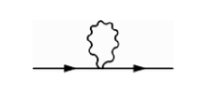
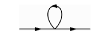
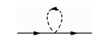
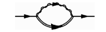
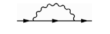
Figure 3: One-loop Feynman diagrams contributing to $\gamma_{Q}$.

Adding the diagrams, we find

$$Z=1+\frac{\lambda}{4\pi^{2}}\,\mathbb{K}\,\ln\Lambda\,$$ (134)

and we read off the matrix of anomalous dimensions,

$$\Gamma^{(1)}\equiv\frac{dZ}{d\ln\Lambda}Z^{-1}=\frac{\lambda}{4\pi^{2}}\,\mathbb{K}\,.$$ (135)

This answer is due entirely to the F-terms, since all other contributions (D-terms, gluon exchange and self-energy diagram) add up to zero. This is an example of a general property of theories with extended supersymmetry [39, 40, 41].

The trace operator is a $4\times 4$ matrix that acts on the four dimensional $\bf{2}\times\bar{\bf{2}}$ vector space $Q^{\cal I}\bar{Q}_{J}$. Its eigenstates are the singlet and the triplet states of $SU(2)_{R}$, with eigenvalues $2$ and $0$ respectively. In this basis the anomalous dimension matrix $\Gamma^{(1)}$ is diagonal, with eigenvalues:

$$\gamma_{\bf{1}}=\frac{\lambda}{2\pi^{2}}\quad\mbox{and}\quad\gamma_{\bf{3}}=0$$ (136)

This result is expected because ${\cal O}_{\bf{3}}$ is an ${\cal N}=2$ chiral primary that obeys the shortening condition $\Delta=2R$, while ${\cal O}_{\bf{1}}$ belongs to a long multiplet and is not protected.

Appendix E Coleman-Weinberg Potential

The calculation of the one-loop effective potential is straightforward but somewhat lengthy. Here we provide some intermediate steps for the sake of the reader who would like to reproduce our result. Following the original paper by Coleman and Weinberg [42], the bosonic and fermionic contributions to the one-loop effective potential are

$${\cal V}_{bose}=\frac{1}{64\pi^{2}}\mbox{Tr}\,{\cal M}_{b}^{4}\ln{\left({\cal M}_{b}^{2}\right)}$$ (137)

$${\cal V}_{fermi}=-\frac{1}{64\pi^{2}}\mbox{Tr}\left({\cal M}_{f}{\cal M}_{f}^{\dagger}\right)^{2}\ln{\left({\cal M}_{f}{\cal M}_{f}^{\dagger}\right)}\,\,,$$ (138)

where the mass matrices read off by expanding the Lagrangian (76) around the classical background. We choose the background (42)

$$Q_{1}=\left(\begin{array}[]{c}q\\ 0\end{array}\right)\,,\quad Q_{2}=\left(\begin{array}[]{c}0\\ -q\end{array}\right)\,,\quad\quad q\in\mathbb{C}\,.$$ (139)

Setting to zero the extra “double-trace” couplings, $f\equiv 0$, we find the following partial contributions (we write $V\equiv v\,\frac{N\,g^{4}\,|q|^{4}}{16\pi^{2}}\,\ln{|q|^{2}}$):

$$v_{Q}=\left(\frac{5+d^{2}(\theta_{1},\theta_{2})}{2}\right)\,\,,$$ (140)

$$v_{fermi}\left(\theta\right)=\left(-\,8+2\,\sin^{2}{\left(\frac{\theta_{1}+\theta_{2}}{2}\right)}+2\,\sin^{2}{\left(\frac{\theta_{1}-\theta_{2}}{2}\right)}\right)\,,$$

$$v_{A}=3\,\,,$$

$$v_{X}=\left(2-2\,\sin^{2}{\left(\frac{\theta_{1}-\theta_{2}}{2}\right)}-2\,\sin^{2}{\left(\frac{\theta_{1}+\theta_{2}}{2}\right)}+4\sin^{2}{\left(\frac{\theta_{1}-\theta_{2}}{2}\right)}\,\sin^{2}{\left(\frac{\theta_{1}+\theta_{2}}{2}\right)}\right)\,.$$

The contribution of the gauge fields is calculated in the Landau gauge. Adding these partial contributions,

$${\cal V}_{1-loop}\left(\theta_{1},\theta_{2};f=0\right)\equiv\frac{\lambda^{2}}{N}\,v_{1-loop}\,|q|^{4}\ln|q|\,$$ (141)

with

$$v_{1-loop}=\frac{1}{8\pi^{2}}\left[4\,\sin^{2}{\left(\frac{\theta_{1}+\theta_{2}}{2}\right)}\sin^{2}{\left(\frac{\theta_{1}-\theta_{2}}{2}\right)}+\frac{d^{2}(\theta_{1},\theta_{2})-1}{2}\right]\,.$$ (142)

For $\theta_{1}=\,\theta_{2}=\theta$, using $d(\theta,\theta)=1$ we find

$${\cal V}_{1-loop}\left(\theta,\theta;f=0\right)=0\,,$$ (143)

as expected since this configuration preserves ${\cal N}=1$ susy.

Along this classical background, the tree-level potential ${\cal V}_{tree}\equiv-({\cal L}_{Q^{4}}+\delta{\cal L}_{fund})$ (see (B.2) and (35)) evaluates to

$${\cal V}_{tree}(q)=\frac{\lambda}{N}\,|q|^{4}\Big{(}1-d(\theta_{1},\theta_{2})\Big{)}+\frac{f_{{\bf 3}^{+}}}{N}\,|q|^{4}\equiv\frac{\lambda}{N}\,{\mathcal{C}}_{\lambda}+\frac{f_{{\bf 3}^{+}}}{N}\,{\mathcal{C}}_{f}\,.$$ (144)

The classical background was chosen precisely to ensure that the only double-trace coupling contributing at tree level is $f_{{\bf 3}^{+}}$. The Callan-Symanzik equation for the effective potential reads

$$\left[\mu\frac{\partial}{\partial\mu}+\beta_{f}\frac{\partial}{\partial f}+\beta_{\lambda}\frac{\partial}{\partial\lambda}-\gamma_{q}^{(1)}\,q\frac{\partial}{\partial q}\right]{\cal V}(q,\mu,f,\lambda)=0\,.$$ (145)

We can drop the $\beta_{\lambda}$ term since it is subleading for large $N$. Writing ${\cal V}(f,\lambda)={\cal V}_{tree}+{\cal V}_{1-loop}(f=0)+O(f)+O(\lambda^{3})$, the CZ equation allows to extract the $f$-independent one-loop coefficient of $\beta_{f}$, $\beta_{f}(f=0)=a(\lambda)=a^{(1)}\lambda^{2}+O(\lambda^{3})$,

$$a^{(1)} = 4\,\gamma_{q}^{(1)}\left({\mathcal{C}}_{\lambda}/{\mathcal{C}}_{f}\right)+v_{1-loop}$$

$$= \frac{1}{16\pi^{2}}\left[\Big{(}1-d(\theta_{1},\theta_{2})\Big{)}+\frac{1}{2}\Big{(}1-d(\theta_{1},\theta_{2})\Big{)}^{2}+4\,\sin^{2}{\left(\frac{\theta_{1}+\theta_{2}}{2}\right)}\sin^{2}{\left(\frac{\theta_{1}-\theta_{2}}{2}\right)}\right]\,.$$

To study the stability of the CW potential, we must first perform the standard RG improvement [42]. A detailed discussion for the problem at hand can be found in section 3 of [21]. One finds that the “perturbative vacuum” $q=0$ is stable if and only if $\beta_{f}$ admits real zeros. In our case $\beta_{f}$ has imaginary zeros and symmetry breaking does occur. This is one of the manifestations of the tachyonic instability on the field theory side.

References

• [1] A. Sen, Tachyon dynamics in open string theory, Int. J. Mod. Phys. A20 (2005) 5513–5656, [hep-th/0410103].
• [2] A. Karch and E. Katz, Adding flavor to AdS/CFT, JHEP 06 (2002) 043, [hep-th/0205236].
• [3] T. Sakai and J. Sonnenschein, Probing flavored mesons of confining gauge theories by supergravity, JHEP 09 (2003) 047, [hep-th/0305049].
• [4] S. Kuperstein, Meson spectroscopy from holomorphic probes on the warped deformed conifold, JHEP 03 (2005) 014, [hep-th/0411097].
• [5] D. Arean, D. E. Crooks, and A. V. Ramallo, Supersymmetric probes on the conifold, JHEP 11 (2004) 035, [hep-th/0408210].
• [6] P. Ouyang, Holomorphic D7-branes and flavored N = 1 gauge theories, Nucl. Phys. B699 (2004) 207–225, [hep-th/0311084].
• [7] F. Canoura, J. D. Edelstein, and A. V. Ramallo, D-brane probes on L(a,b,c) superconformal field theories, JHEP 09 (2006) 038, [hep-th/0605260].
• [8] R. Apreda, J. Erdmenger, D. Lust, and C. Sieg, Adding flavour to the Polchinski-Strassler background, JHEP 01 (2007) 079, [hep-th/0610276].
• [9] C. Sieg, Holographic flavour in the N = 1 Polchinski-Strassler background, JHEP 08 (2007) 031, [0704.3544].
• [10] S. Penati, M. Pirrone, and C. Ratti, Mesons in marginally deformed AdS/CFT, JHEP 04 (2008) 037, [0710.4292].
• [11] X.-J. Wang and S. Hu, Intersecting branes and adding flavors to the Maldacena- Nunez background, JHEP 09 (2003) 017, [hep-th/0307218].
• [12] C. Nunez, A. Paredes, and A. V. Ramallo, Flavoring the gravity dual of N = 1 Yang-Mills with probes, JHEP 12 (2003) 024, [hep-th/0311201].
• [13] A. Karch and L. Randall, Open and closed string interpretation of SUSY CFT’s on branes with boundaries, JHEP 06 (2001) 063, [hep-th/0105132].
• [14] O. DeWolfe, D. Z. Freedman, and H. Ooguri, Holography and defect conformal field theories, Phys. Rev. D66 (2002) 025009, [hep-th/0111135].
• [15] J. Erdmenger, Z. Guralnik, and I. Kirsch, Four-Dimensional Superconformal Theories with Interacting Boundaries or Defects, Phys. Rev. D66 (2002) 025020, [hep-th/0203020].
• [16] K. Skenderis and M. Taylor, Branes in AdS and pp-wave spacetimes, JHEP 06 (2002) 025, [hep-th/0204054].
• [17] N. R. Constable, J. Erdmenger, Z. Guralnik, and I. Kirsch, Intersecting D3-branes and holography, Phys. Rev. D68 (2003) 106007, [hep-th/0211222].
• [18] A. Adams and E. Silverstein, Closed string tachyons, AdS/CFT, and large N QCD, Phys. Rev. D64 (2001) 086001, [hep-th/0103220].
• [19] A. Dymarsky, I. R. Klebanov, and R. Roiban, Perturbative gauge theory and closed string tachyons, JHEP 11 (2005) 038, [hep-th/0509132].
• [20] A. Dymarsky, I. R. Klebanov, and R. Roiban, Perturbative search for fixed lines in large N gauge theories, JHEP 08 (2005) 011, [hep-th/0505099].
• [21] E. Pomoni and L. Rastelli, Large N Field Theory and AdS Tachyons, 0805.2261.
• [22] P. Breitenlohner and D. Z. Freedman, Positive Energy in anti-De Sitter Backgrounds and Gauged Extended Supergravity, Phys. Lett. B115 (1982) 197.
• [23] N. Marcus, A. Sagnotti, and W. Siegel, TEN-DIMENSIONAL SUPERSYMMETRIC YANG-MILLS THEORY IN TERMS OF FOUR-DIMENSIONAL SUPERFIELDS, Nucl. Phys. B224 (1983) 159.
• [24] S. J. Gates, M. T. Grisaru, M. Rocek, and W. Siegel, Superspace, or one thousand and one lessons in supersymmetry, Front. Phys. 58 (1983) 1–548, [hep-th/0108200].
• [25] O. Aharony, A. Fayyazuddin, and J. M. Maldacena, The large N limit of N = 2,1 field theories from three- branes in F-theory, JHEP 07 (1998) 013, [hep-th/9806159].
• [26] M. Kruczenski, D. Mateos, R. C. Myers, and D. J. Winters, Meson spectroscopy in AdS/CFT with flavour, JHEP 07 (2003) 049, [hep-th/0304032].
• [27] F. T. J. Epple and D. Lust, Tachyon condensation for intersecting branes at small and large angles, Fortsch. Phys. 52 (2004) 367–387, [hep-th/0311182].
• [28] N. Berkovits, A Ten-dimensional superYang-Mills action with off-shell supersymmetry, Phys. Lett. B318 (1993) 104–106, [hep-th/9308128].
• [29] L. Baulieu, N. J. Berkovits, G. Bossard, and A. Martin, Ten-dimensional super-Yang-Mills with nine off-shell supersymmetries, Phys. Lett. B658 (2008) 249–254, [0705.2002].
• [30] L. J. Dixon, D. Friedan, E. J. Martinec, and S. H. Shenker, The Conformal Field Theory of Orbifolds, Nucl. Phys. B282 (1987) 13–73.
• [31] M. Cvetic and I. Papadimitriou, Conformal field theory couplings for intersecting D-branes on orientifolds, Phys. Rev. D68 (2003) 046001, [hep-th/0303083].
• [32] S. A. Abel and A. W. Owen, Interactions in intersecting brane models, Nucl. Phys. B663 (2003) 197–214, [hep-th/0303124].
• [33] I. Antoniadis, K. Benakli, and A. Laugier, Contact interactions in D-brane models, JHEP 05 (2001) 044, [hep-th/0011281].
• [34] T. Erler and N. Mann, Integrable open spin chains and the doubling trick in N = 2 SYM with fundamental matter, JHEP 01 (2006) 131, [hep-th/0508064].
• [35] N. Mann and S. E. Vazquez, Classical open string integrability, JHEP 04 (2007) 065, [hep-th/0612038].
• [36] D. H. Correa and C. A. S. Young, Reflecting magnons from D7 and D5 branes, J. Phys. A41 (2008) 455401, [0808.0452].
• [37] D. H. Correa and C. A. S. Young, Asymptotic Bethe equations for open boundaries in planar AdS/CFT, 0912.0627.
• [38] J. A. Minahan and K. Zarembo, The Bethe-ansatz for N = 4 super Yang-Mills, JHEP 03 (2003) 013, [hep-th/0212208].
• [39] E. D’Hoker, D. Z. Freedman, and W. Skiba, Field theory tests for correlators in the AdS/CFT correspondence, Phys. Rev. D59 (1999) 045008, [hep-th/9807098].
• [40] N. R. Constable et al., PP-wave string interactions from perturbative Yang-Mills theory, JHEP 07 (2002) 017, [hep-th/0205089].
• [41] E. D’Hoker and A. V. Ryzhov, Three-point functions of quarter BPS operators in N = 4 SYM, JHEP 02 (2002) 047, [hep-th/0109065].
• [42] S. R. Coleman and E. Weinberg, Radiative Corrections as the Origin of Spontaneous Symmetry Breaking, Phys. Rev. D7 (1973) 1888–1910.