Directional Dynamics along Arbitrary Curves
in Cellular Automata

Abstract

This paper studies directional dynamics on one-dimensional cellular automata, a formalism previously introduced by the third author. The central idea is to study the dynamical behaviour of a cellular automaton through the conjoint action of its global rule (temporal action) and the shift map (spacial action): qualitative behaviours inherited from topological dynamics (equicontinuity, sensitivity, expansivity) are thus considered along arbitrary curves in space-time. The main contributions of the paper concern equicontinuous dynamics which can be connected to the notion of consequences of a word. We show that there is a cellular automaton with an equicontinuous dynamics along a parabola, but which is sensitive along any linear direction. We also show that real numbers that occur as the slope of a limit linear direction with equicontinuous dynamics in some cellular automaton are exactly the computably enumerable numbers.

Introduction

Introduced by J. von Neumann as a computational device, cellular automata (CA) were also studied as a model of dynamical systems [7]. G. A. Hedlund et al. gave a characterization of CA through their global action on configurations: they are exactly the continuous and shift-commuting maps acting on the (compact) space of configurations. Since then, CA were extensively studied as discrete time dynamical systems for their remarkable general properties (e.g., injectivity implies surjectivity) but also through the lens of topological dynamics and deterministic chaos. With this latter point of view, P. Kůrka [9] has proposed a classification of 1D CA according to their equicontinuous properties (see [12] for a similar classification in higher dimensions). As often remarked in the literature, the limitation of this approach is to not take into account the shift-invariance of CA: information flow is rigidly measured with respect to a particular reference cell which does not vary with time and, for instance, the shift map is considered as sensitive to initial configurations.

One significant step to overcome this limitation was accomplished with the formalism of directional dynamics recently proposed by M. Sablik [11]. The key idea is to consider the action of the rule and that of the shift simultaneously. CA are thus seen as $\mathbb{Z}^{2}$-actions (or $\mathbb{N}\times\mathbb{Z}$-actions for irreversible rules). In [11], each qualitative behaviour of Kůrka’s classification (equicontinuity, sensitivity, expansivity) is considered for different linear correlations between the two components of the $\mathbb{Z}^{2}$-action corresponding to different linear directions in space-time. For a fixed direction the situation is similar to Kůrka’s classification, but in [11], the classification scheme consists in discussing what sets of directions support each qualitative behaviour.

The restriction to linear directions is natural, but [11] asks whether considering non-linear directions can be useful. One of the main points of the present paper is to give a positive response to this question. We are going to study each qualitative behaviour along arbitrary curves in space-time and show that, in some CA, a given behaviour appears along some non-linear curve but not along any linear direction. Another contribution of the paper is to give a complete characterization of real numbers that can occur as (limit) linear directions for equicontinuous dynamics.

Properties inherited from classical topological dynamics may have a concrete interpretation when applied to CA. In particular, as remarked by P. Kůrka, the existence of equicontinuity points is equivalent to the existence of a ’wall’, that is a word whose presence in the initial configuration implies an infinite strip of consequences in space-time (a portion of the lattice has a determined value at each time step whatever the value of the configuration outside the ’wall’). In our context, the connection between equicontinuous dynamics and consequences of a word still apply but in a broader sense since we consider arbitrary curves in space-time. The examples of dynamic behaviour along non-trivial curves built in this paper will often rely on particular words whose set of consequences have the desired shape.

Another way of looking at the notion of consequences of a word is to use the analogy of information propagation and signals already developed in the field of classical algorithmics in CA [13]. From that point of view, a word whose consequences follow a given curve in space-time can be seen as a signal which is robust to any pertubations from the context. Thus, many of our results can be seen as constructions in a non-standard algorithmic framework where information propagation must be robust to any context. To achieve our results, we have developed general mechanisms to introduce a form of robustness (counter technique, section 3). We believe that, besides the results we obtain, this technique is of some interest on its own.

After the next section, aimed at recalling useful definitions, the paper is organized in four parts as follows:

• in section 2, we extend the theory of directional dynamics to arbitrary curves and prove a classification theorem analogue to that of [11];

• in section 3, we focus on equicontinuous dynamics and give constructions and construction tools; the main result is the existence of various CA where equicontinuous dynamics occur along some curve but not along others and particularly not along any linear direction;

• in section 4, we focus on linear directions corresponding to equicontinuous dynamics; [11] showed that the set of slopes of such linear directions is an interval (if not empty): we give a characterisation of real numbers that can occur as bounds of such intervals.

• in section 5, we give some negative results concerning possible sets of consequences of a word in CA; in particular, we show how the set of curves admitting equicontinuous dynamics is constrained in reversible CA.

1 Some definitions

1.1 Space considerations

Configuration space

Let $\mathcal{A}$ be a finite set and $\mathcal{A}^{\mathbb{Z}}$ the configuration space of $\mathbb{Z}$-indexed sequences in $\mathcal{A}$. If $\mathcal{A}$ is endowed with the discrete topology, $\mathcal{A}^{\mathbb{Z}}$ is metrizable, compact and totally disconnected in the product topology. A compatible metric is given by:

$$\forall x,y\in\mathcal{A}^{\mathbb{Z}},\quad d_{C}(x,y)=2^{-\min\{|i|:x_{i}\neq y_{i}\ i\in\mathbb{Z}\}}.$$

Consider a not necessarily convex subset $\mathbb{U}\subset\mathbb{Z}$. For $x\in\mathcal{A}^{\mathbb{Z}}$, denote $x_{\mathbb{U}}\in\mathcal{A}^{\mathbb{U}}$ the restriction of $x$ to $\mathbb{U}$. Given $w\in\mathcal{A}^{\mathbb{U}}$, one defines the cylinder centered at $w$ by $[w]_{\mathbb{U}}=\{x\in\mathcal{A}^{\mathbb{Z}}:x_{\mathbb{U}}=w\}$. Denote by $\mathcal{A}^{\ast}$ the set of all finite sequences or finite words $w=w_{0}...w_{n-1}$ with letters in $\mathcal{A}$; $|w|=n$ is the length of $w$. When there is no ambiguity, denote $[w]_{i}=[w]_{\llbracket i,i+|w|-1\rrbracket}$.

Shift action

The shift map $\sigma:\mathcal{A}^{\mathbb{Z}}\rightarrow\mathcal{A}^{\mathbb{Z}}$ is defined by $\sigma(x)_{i}=x_{i+1}$ for $x=(x_{m})_{m\in\mathbb{Z}}\in\mathcal{A}^{\mathbb{Z}}$ and $i\in\mathbb{Z}$. It is a homeomorphism of $\mathcal{A}^{\mathbb{Z}}$.

A closed and $\sigma$-invariant subset $\Sigma$ of $\mathcal{A}^{\mathbb{Z}}$ is called a subshift. For $\mathbb{U}\subset\mathbb{Z}$ denote $\mathcal{L}_{\Sigma}(\mathbb{U})=\{x_{\mathbb{U}}:x\in\Sigma\}$ the set of patterns centered at $\mathbb{U}$. Since $\Sigma$ is $\sigma$-invariant, it is sufficient to consider the words of length $n\in\mathbb{N}$ for a suitable $n$. We denote $\mathcal{L}_{\Sigma}(n)=\{x_{\llbracket 0,n-1\rrbracket}:x\in\Sigma\}$. The language of a subshift $\Sigma$ is defined by $\mathcal{L}_{\Sigma}=\cup_{n\in\mathbb{N}}\mathcal{L}_{\Sigma}(n)$. By compactness, the language characterizes the subshift.

A subshift $\Sigma\subseteq\mathcal{A}^{\mathbb{Z}}$ is transitive if given words $u,v\in\mathcal{L}_{\Sigma}$ there is $w\in\mathcal{L}_{\Sigma}$ such that $uwv\in\mathcal{L}_{\Sigma}$. It is mixing if given $u,v\in\mathcal{L}_{\Sigma}$ there is $N\in\mathbb{N}$ such that $uwv\in\mathcal{L}_{\Sigma}$ for any $n\geq N$ and some $w\in\mathcal{L}_{\Sigma}(n)$.

A subshift $\Sigma\subset\mathcal{A}^{\mathbb{Z}}$ is specified if there exists $N\in\mathbb{N}$ such that for all $u,v\in\mathcal{L}_{\Sigma}$ and for all $n\geq N$ there exists a $\sigma$-periodic point $x\in\Sigma$ such that $x_{\llbracket 0,|u|-1\rrbracket}=u$ and $x_{\llbracket n+|u|,n+|u|+|v|-1\rrbracket}=v$ (see [4] for more details).

A subshift $\Sigma\subset\mathcal{A}^{\mathbb{Z}}$ is weakly-specified if there exists $N\in\mathbb{N}$ such that for all $u,v\in\mathcal{L}_{\Sigma}$ there exist $n\leq N$ and a $\sigma$-periodic point $x\in\Sigma$ such that $x_{\llbracket 0,|u|-1\rrbracket}=u$ and $x_{\llbracket n+|u|,n+|u|+|v|-1\rrbracket}=v$.

Specification (resp. weakly-specification) implies mixing (resp. transitivity) and density of $\sigma$-periodic points. Let $\Sigma$ be a weakly-specified mixing subshift. By compactness there exists $N\in\mathbb{N}$ such that for any $x,y\in\Sigma$ and $i\in\mathbb{N}$ there exist $w\in\mathcal{L}_{\Sigma}$, $|w|\leq N$, and $j\in\mathbb{Z}$ such that $x_{\rrbracket-\infty,i\rrbracket}w\sigma^{j}(y)_{\llbracket i+|w|,\infty\llbracket}\in\Sigma$. If $\Sigma$ is specified this property is true with $|w|=n$ and $n\geq N$.

Subshifts of finite type and sofic subshifts

A subshift $\Sigma$ is of finite type if there exist a finite subset $\mathbb{U}\subset\mathbb{Z}$ and $\mathcal{F}\subset\mathcal{A}^{\mathbb{U}}$ such that $x\in\Sigma$ if and only if $\sigma^{m}(x)_{\mathbb{U}}\in\mathcal{F}$ for all $m\in\mathbb{Z}$. The diameter of $\mathbb{U}$ is called an order of $\Sigma$.

A subshift $\Sigma^{\prime}\subset\mathcal{B}^{\mathbb{Z}}$ is sofic if it is the image of a subshift of finite type $\Sigma\subset\mathcal{A}^{\mathbb{Z}}$ by a map $\pi:\mathcal{A}^{\mathbb{Z}}\to\mathcal{B}^{\mathbb{Z}}$, $\pi((x_{i})_{i\in{\mathbb{Z}}})=(\pi(x_{i}))_{i\in\mathbb{Z}}$, where $\pi:\mathcal{A}\to\mathcal{B}$.

A transitive sofic subshift is weakly-specified and a mixing sofic subshift is specified. For precise statements and proofs concerning sofic subshifts and subshifts of finite type see [10] or [8].

1.2 Time considerations

Cellular automata

A cellular automaton (CA) is a dynamical system $(\mathcal{A}^{\mathbb{Z}},F)$ defined by a local rule which acts uniformly and synchronously on the configuration space. That is, there are a finite segment or neighborhood $\mathbb{U}\subset\mathbb{Z}$ and a local rule $\overline{F}:\mathcal{A}^{\mathbb{U}}\rightarrow\mathcal{A}$ such that $F(x)_{m}=\overline{F}((x_{m+u})_{u\in\mathbb{U}})$ for all $x\in\mathcal{A}^{\mathbb{Z}}$ and $m\in\mathbb{Z}$. The radius of $F$ is $r(F)=\max\{|u|:u\in\mathbb{U}\}$. By Hedlund’s theorem [7], a cellular automaton is equivalently defined as a pair $(\mathcal{A}^{\mathbb{Z}},F)$ where $F:\mathcal{A}^{\mathbb{Z}}\to\mathcal{A}^{\mathbb{Z}}$ is a continuous function which commutes with the shift.

Considering the past: bijective CA

When the CA is bijective, since $\mathcal{A}^{\mathbb{Z}}$ is compact, $F^{-1}$ is also a continuous function which commutes with $\sigma$. By Hedlund’s theorem, $(\mathcal{A}^{\mathbb{Z}},F^{-1})$ is then also a CA (however the radius of $F^{-1}$ can be much larger than that of $F$). In this case one can study the $\mathbb{Z}$-action $F$ on $\mathcal{A}^{\mathbb{Z}}$ and not only $F$ as an $\mathbb{N}$-action. This means that we can consider positive (future) and negative (past) iterates of a configuration.

Thus, if the CA is bijective, we can study the dynamic of the CA as an $\mathbb{N}$-action or a $\mathbb{Z}$-action. In the general case, we consider the $\mathbb{K}$-action of a CA where $\mathbb{K}$ can be $\mathbb{N}$ or $\mathbb{Z}$.

1.3 A CA as a $\mathbb{Z}\times\mathbb{K}$-action

Space-time diagrams

Let $(\mathcal{A}^{\mathbb{Z}},F)$ be a CA, since $F$ commutes with the shift $\sigma$, we can consider the $\mathbb{Z}\times\mathbb{K}$-action $(\sigma,F)$. For $x\in\mathcal{A}^{\mathbb{Z}}$, we denote by ${\langle m,n\rangle_{\sigma,F}(x)=\bigl{(}\sigma^{m}\circ F^{n}(x)\bigr{)}_{0}}$ the color of the site $\langle m,n\rangle\in\mathbb{Z}\times\mathbb{K}$ generated by $x$.

Adopting a more geometrical point of view, we also refer to this coloring of $\mathbb{Z}\times\mathbb{K}$ as the space-time diagram generated by $x$.

Region of consequences

Let $X\subset\mathcal{A}^{\mathbb{Z}}$ be any set of configurations. We define the region of consequences of $X$ by:

$$\mathfrak{C}_{F}(X)=\left\{\langle m,n\rangle\in\mathbb{Z}\times\mathbb{K}:\forall x,y\in X\textrm{ one has }\langle m,n\rangle_{\sigma,F}(x)=\langle m,n\rangle_{\sigma,F}(y)\right\}.$$

This set corresponds to the sites that are fixed by all $x\in X$ under the $\mathbb{Z}\times\mathbb{K}$-action $(\sigma,F)$, or equivalently, sites which are identically colored in all space-time diagrams generated by some $x\in X$. The main purpose of this article is to study this set and make links with notions from topological dynamics.

Let $(\mathcal{A}^{\mathbb{Z}},F)$ be a CA of neighborhood $\mathbb{U}=\llbracket r,s\rrbracket$ and let $u\in\mathcal{A}^{+}$. An example of such set $X$ that will be used throughout the paper is $[u]_{0}$. Trivially, one has (see figure 1)

$$\left\{\langle m,n\rangle:nr\leq m<|u|-ns\right\}\subseteq\mathfrak{C}_{F}([u]_{0})\subseteq\left\{\langle m,n\rangle:-nr\leq m<|u|+ns\right\}$$

In the sequel, we often call $\mathfrak{C}_{F}([u]_{0})$ the cone of consequences of $u$. Note that the inclusions above do not tell whether $\mathfrak{C}_{F}([u]_{0})$ is finite or infinite.

Figure 1: Consequences of a word $u$.

2 Dynamics along an arbitrary curve

In this section, we define sensitivity to initial conditions along a curve and we establish a connection with cones of consequences. What we call a curve is simply a map $h:\mathbb{K}\rightarrow\mathbb{Z}$ giving a position in space for each time step. Such $h$ can be arbitrary in the following definitions, but later in the paper we will put restrictions on them to adapt to the local nature of cellular automata.

2.1 Sensitivity to initial conditions along a curve

Let $\Sigma$ be a subshift of $\mathcal{A}^{\mathbb{Z}}$ and assume $\mathbb{K}=\mathbb{N}$ or $\mathbb{Z}$.

Let $x\in\Sigma$, $\varepsilon>0$ and $h:\mathbb{K}\to\mathbb{Z}$. The ball (relative to $\Sigma$) centered at $x$ of radius $\varepsilon$ is given by $B_{\Sigma}(x,\varepsilon)=\{y\in\Sigma:d_{C}(x,y)<\varepsilon\}$ and the tube along $h$ centered at $x$ of radius $\varepsilon$ is (see figure 2):

$$D^{h}_{\Sigma}(x,\varepsilon,\mathbb{K})=\{y\in\Sigma:d_{C}(\sigma^{h(n)}\circ F^{n}(x),\sigma^{h(n)}\circ F^{n}(y))<\varepsilon,\forall n\in\mathbb{K}\}.$$

Notice that one can define a distance $D(x,y)=\sup(\{d_{C}(\sigma^{h(n)}\circ F^{n}(x),\sigma^{h(n)}\circ F^{n}(y)):\forall n\in\mathbb{N}\})$ for all $x,y\in\Sigma$. The tube $D^{h}_{\Sigma}(x,\varepsilon,\mathbb{K})$ is then nothing else than the open ball of radius $\varepsilon$ centered at $x$.

Figure 2: Tube along $h$ of width $\varepsilon$ centered at $x$. The gray region is where $F^{n}(x)$ and $F^{n}(y)$ must match.

If the CA is bijective, one can assume that $\mathbb{K}=\mathbb{Z}$.

Definition 2.1.

Assume $\mathbb{K}=\mathbb{N}$ or $\mathbb{Z}$. Let $(\mathcal{A}^{\mathbb{Z}},F)$ be a CA, $\Sigma\subset\mathcal{A}^{\mathbb{Z}}$ be a subshift and $h:\mathbb{K}\to\mathbb{Z}$.

• The set $Eq^{h}_{\mathbb{K}}(\Sigma,F)$ of $(\mathbb{K},\Sigma)$-equicontinuous points along $h$ is defined by

  $$x\in Eq^{h}_{\mathbb{K}}(\Sigma,F)\Longleftrightarrow\forall\varepsilon>0,\exists\delta>0,\ B_{\Sigma}(x,\delta)\subset D^{h}_{\Sigma}(x,\varepsilon,\mathbb{K}).$$

• $(\mathcal{A}^{\mathbb{Z}},F)$ is (uniformly) $(\mathbb{K},\Sigma)$-equicontinuous along $h$ if

  $$\forall\varepsilon>0,\exists\delta>0,\forall x\in\Sigma,\ B_{\Sigma}(x,\delta)\subset D^{h}_{\Sigma}(x,\varepsilon,\mathbb{K}).$$

• $(\mathcal{A}^{\mathbb{Z}},F)$ is $(\mathbb{K},\Sigma)$-sensitive along $h$ if

  $$\exists\varepsilon>0,\forall\delta>0,\forall x\in\Sigma,\ \exists y\in B_{\Sigma}(x,\delta)\smallsetminus D^{h}_{\Sigma}(x,\varepsilon,\mathbb{K}).$$

• $(\mathcal{A}^{\mathbb{Z}},F)$ is $(\mathbb{K},\Sigma)$-expansive along $h$ if

  $$\exists\varepsilon>0,\forall x\in\Sigma,\ D^{h}_{\Sigma}(x,\varepsilon,\mathbb{K})=\{x\}.$$

Since the domain of a CA is a two sided fullshift, it is possible to break up the concept of expansivity into right-expansivity and left-expansivity. The intuitive idea is that ‘information” can move by the action of a CA to the right and to the left.

1. $(\mathcal{A}^{\mathbb{Z}},F)$ is $(\mathbb{K},\Sigma)$-right-expansive along $h$ if there exists $\varepsilon>0$ such that $D_{\Sigma}^{h}(x,\varepsilon,\mathbb{K})\cap D_{\Sigma}^{h}(y,\varepsilon,\mathbb{K})=\emptyset$ for all $x,y\in\Sigma$ such that $x_{\llbracket 0,+\infty\llbracket}\neq y_{\llbracket 0,+\infty\llbracket}$.

2. $(\mathcal{A}^{\mathbb{Z}},F)$ is $(\mathbb{K},\Sigma)$-left-expansive along $h$ if there exists $\varepsilon>0$ such that $D_{\Sigma}^{h}(x,\varepsilon,\mathbb{K})\cap D_{\Sigma}^{h}(y,\varepsilon,\mathbb{K})=\emptyset$ for all $x,y\in\Sigma$ such that $x_{\rrbracket-\infty,0\rrbracket}\neq y_{\rrbracket-\infty,0\rrbracket}$.

Thus the CA $(\mathcal{A}^{\mathbb{Z}},F)$ is $(\mathbb{K},\Sigma)$-expansive along $h$ if it is both $(\mathbb{K},\Sigma)$-left-expansive and $(\mathbb{K},\Sigma)$-right-expansive along $h$.

For $\alpha\in\mathbb{R}$, define:

$$\begin{array}[]{llll}h_{\alpha}:&\mathbb{K}&\longrightarrow&\mathbb{Z}\\ &n&\longmapsto&\lfloor\alpha n\rfloor.\end{array}$$

Thus, dynamics along $\alpha$ introduced in [11] correspond to dynamics along $h_{\alpha}$ defined in this paper.

2.2 Blocking words for functions with bounded variation

To translate equicontinuity concepts into space-time diagrams properties, we need the notion of blocking word along $h$. The wall generated by a blocking word can be interpreted as a particle which has the direction $h$ and kills any information coming from the right or the left. For that we need that the variation of the function $h$ is bounded.

Definition 2.2.

The set of functions with bounded variation is defined by:

$$\mathcal{F}=\left\{h:\mathbb{K}\to\mathbb{Z}:\exists M>0,\ \forall n\in\mathbb{K},\ |h(n+1)-h(n)|\leq M\right\}.$$

Note that $\mathcal{F}$ depends on $\mathbb{K}$, but we will never make this explicit and the context will always make this notation unambiguous in the sequel.

Definition 2.3.

Assume $\mathbb{K}=\mathbb{N}$ or $\mathbb{Z}$. Let $(\mathcal{A}^{\mathbb{Z}},F)$ be a CA with neighborhood $\mathbb{U}=\llbracket r,s\rrbracket$ (same neighborhood for $F^{-1}$ if $\mathbb{K}=\mathbb{Z}$).

Let $\Sigma\subset\mathcal{A}^{\mathbb{Z}}$ be a subshift, $h\in\mathcal{F}$, $e\in\mathbb{N}$ such that

$$e>\max_{n\in\mathbb{K}}(|h(n+1)-h(n)|+s,|h(n+1)-h(n)|-r)$$

and $u\in\mathcal{L}_{\Sigma}$ with $|u|\geq e$. The word $u$ is a $(\mathbb{K},\Sigma)$-blocking word along $h$ and width $e$ if there exists a $p\in\mathbb{Z}$ such that (see figure 3):

$$\mathfrak{C}_{F}(\Sigma\cap[u]_{p})\supset\left\{\langle m,n\rangle\in\mathbb{Z}\times\mathbb{K}:h(n)\leq m<h(n)+e\right\}.$$

Figure 3: Blocking word $u$ of width $e$ for a CA of neighborhood $\llbracket r,s\rrbracket$. The gray region represents the consequences of $u$.

The evolution of a cell $i\in\mathbb{Z}$ depends on the cells $\llbracket i+r,i+s\rrbracket$. Thus, due to condition on $e$, it is easy to deduce that if $u$ is a $(\mathbb{K},\Sigma)$-blocking word along $h$ and width $e$, then for all $j\in\mathbb{Z}$, $x,y\in[u]_{j}\cap\Sigma$ such that $x_{\rrbracket-\infty,j\rrbracket}=y_{\rrbracket-\infty,j\rrbracket}$ and $n\in\mathbb{K}$ one has $F^{n}(x)_{i}=F^{n}(y)_{i}$ for $i\leq h(n)+p+e+j$. Similarly for all $x,y\in[u]_{j}\cap\Sigma$ such that $x_{\llbracket j,\infty\llbracket}=y_{\llbracket j,\infty\llbracket}$, one has $F^{n}(x)_{i}=F^{n}(y)_{i}$ for all $i\geq h(n)+p$. Intuitively, no information can cross the wall along $h$ and width $e$ generated by the $(\mathbb{K},\Sigma)$-blocking word.

The proof of the classification of CA given in [9] can be easily adapted to obtain a characterization of CA which have equicontinuous points along $h$.

Proposition 2.1.

Assume $\mathbb{K}=\mathbb{N}$ or $\mathbb{Z}$. Let $(\mathcal{A}^{\mathbb{Z}},F)$ be a CA, $\Sigma\subset\mathcal{A}^{\mathbb{Z}}$ be a transitive subshift and $h\in\mathcal{F}$. The following properties are equivalent:

1. $(\mathcal{A}^{\mathbb{Z}},F)$ is not $(\mathbb{K},\Sigma)$-sensitive along $h$;

2. $(\mathcal{A}^{\mathbb{Z}},F)$ has a $(\mathbb{K},\Sigma)$-blocking word along $h$;

3. $Eq^{h}_{\mathbb{K}}(\Sigma,F)\neq\emptyset$ is a $\sigma$-invariant dense $G_{\delta}$ set.

Proof.

Let $\mathbb{U}=\llbracket r,s\rrbracket$ be a neighborhood of $F$ (and also of $F^{-1}$ if $\mathbb{K}=\mathbb{Z}$).

$(1)\Rightarrow(2)$ Let $e\geq\max_{n\in\mathbb{K}}(|h(n+1)-h(n)|+1+s,|h(n+1)-h(n)|+1-r)$. If $(\mathcal{A}^{\mathbb{Z}},F)$ is not $(\mathbb{K},\Sigma)$-sensitive along $h$, then there exist $x\in\Sigma$ and $k,p\in\mathbb{N}$ such that for all $y\in\Sigma$ verifying $x_{\llbracket 0,k\rrbracket}=y_{\llbracket 0,k\rrbracket}$ one has:

$$\forall n\in\mathbb{K},\ \sigma^{h(n)}\circ F^{n}(x)_{\llbracket p,p+e-1\rrbracket}=\sigma^{h(n)}\circ F^{n}(y)_{\llbracket p,p+e-1\rrbracket}.$$

Thus $x_{\llbracket 0,k\rrbracket}$ is a $(\mathbb{K},\Sigma)$-blocking word along $h$ and width $e$.

$(2)\Rightarrow(3)$ Let $u$ be a $(\mathbb{K},\Sigma)$-blocking word along $h$. Since $(\Sigma,\sigma)$ is transitive, then there exists $x\in\Sigma$ containing an infinitely many occurrences of $u$ in positive and negative coordinates. Let $k\in\mathbb{N}$. There exists $k_{1}\geq k$ and $k_{2}\geq k$ such that $x_{\llbracket-k_{1},-k_{1}+|u|-1\rrbracket}=x_{\llbracket k_{2},k_{2}+|u|-1\rrbracket}=u$. Since $u$ is a $(\mathbb{K},\Sigma)$-blocking word along $h$, for all $y\in\Sigma$ such that $y_{\llbracket-k_{1},k_{2}+|u|-1\rrbracket}=x_{\llbracket-k_{1},k_{2}+|u|-1\rrbracket}$ one has

$$\sigma^{h(n)}\circ F^{n}(x)_{\llbracket-k,k\rrbracket}=\sigma^{h(n)}\circ F^{n}(y)_{\llbracket-k,k\rrbracket}\quad\forall n\in\mathbb{K}.$$

One deduces that $x\in Eq^{h}_{\mathbb{K}}(\Sigma,F)$.

Moreover, since $\Sigma$ is transitive, the subset of points in $\Sigma$ containing infinitely many occurrences of $u$ in positive and negative coordinates is a $\sigma$-invariant dense $G_{\delta}$ set of $\Sigma$.

$(3)\Rightarrow(1)$ Follows directly from definitions. ∎

Remark 2.1.

When $\Sigma$ is not transitive one can show that any $(\mathbb{K},\Sigma)$-equicontinuous point along $h$ contains a $(\mathbb{K},\Sigma)$-blocking word along $h$. Reciprocally, a point $x\in\Sigma$ containing infinitely many occurrences of a $(\mathbb{K},\Sigma)$-blocking word along $h$ in positive and negative coordinates is a $(\mathbb{K},\Sigma)$-equicontinuous point along $h$. However, if $\Sigma$ is not transitive, the existence of a $(\mathbb{K},\Sigma)$-blocking word does not imply that one can repeat it infinitely many times.

2.3 A classification following a curve

Thanks to Proposition 2.1 it is possible to establish a classification as in [9], but following a given curve.

Theorem 2.2.

Assume $\mathbb{K}=\mathbb{N}$ or $\mathbb{Z}$. Let $(\mathcal{A}^{\mathbb{Z}},F)$ be a CA, $\Sigma\subset\mathcal{A}^{\mathbb{Z}}$ be a transitive subshift and $h\in\mathcal{F}$. One of the following cases holds:

1. $Eq^{h}_{\mathbb{K}}(\Sigma,F)=\Sigma$ $\Longleftrightarrow$ $(\mathcal{A}^{\mathbb{Z}},F)$ is $(\mathbb{K},\Sigma)$-equicontinuous along $h$;

2. $\emptyset\neq Eq^{h}_{\mathbb{K}}(\Sigma,F)\neq\Sigma$ $\Longleftrightarrow$ $(\mathcal{A}^{\mathbb{Z}},F)$ is not $(\mathbb{K},\Sigma)$-sensitive along $h$ $\Longleftrightarrow$ $(\Sigma,F)$ has a $(\mathbb{K},\Sigma)$-blocking word along $h$;

3. $(\mathcal{A}^{\mathbb{Z}},F)$ is $(\mathbb{K},\Sigma)$-sensitive along $h$ but is not $(\mathbb{K},\Sigma)$-expansive along $h$;

4. $(\mathcal{A}^{\mathbb{Z}},F)$ is $(\mathbb{K},\Sigma)$-expansive along $h$.

Proof.

First we prove the first equivalence. From definitions we deduce that if $(\mathcal{A}^{\mathbb{Z}},F)$ is $(\mathbb{K},\Sigma)$-equicontinuous along $h$ then $Eq^{h}_{\mathbb{K}}(\Sigma,F)=\Sigma$. In the other direction, consider the distance $D(x,y)=\sup(\{d_{C}(\sigma^{h(n)}\circ F^{n}(x),\sigma^{h(n)}\circ F^{n}(y)):\forall n\in\mathbb{N}\})$ mentionned earlier. $Eq^{h}_{\mathbb{K}}(\Sigma,F)$ is the set of equicontinuous points of the function $\mathrm{Id}:(\Sigma,d_{C})\to(\Sigma,D)$. By compactness, if this function is continuous on $\Sigma$, then it is uniformly continuous. One deduces that $(\mathcal{A}^{\mathbb{Z}},F)$ is $(\mathbb{K},\Sigma)$-equicontinuous along $h$.

The second equivalence and the classification follow directly from Proposition 2.1. ∎

2.4 Sets of curves with a certain kind of dynamics

We are going to study the sets of curves along which a certain kind of dynamics happens. We obtain a classification similar at the classification obtained in [11] but not restricted to linear directions.

Definition 2.4.

Assume $\mathbb{K}=\mathbb{N}$ or $\mathbb{Z}$. Let $(\mathcal{A}^{\mathbb{Z}},F)$ be a CA and $\Sigma$ be a subshift. We define the following sets of curves.

• Sets corresponding to topological equicontinuous properties:

  $$\textbf{A}_{\mathbb{K}}(\Sigma,F) = \{h\in\mathcal{F}:Eq^{h}_{\mathbb{K}}(\Sigma,F)\neq\emptyset\},$$

  $$\textrm{and }\textbf{A}_{\mathbb{K}}^{\prime}(\Sigma,F) = \{h\in\mathcal{F}:Eq^{h}_{\mathbb{K}}(\Sigma,F)=\Sigma\}.$$

  One has $\textbf{A}_{\mathbb{K}}^{\prime}(\Sigma,F)\subset\textbf{A}_{\mathbb{K}}(\Sigma,F).$

• Sets corresponding to topological expansive properties:

  $$\textbf{B}_{\mathbb{K}}(\Sigma,F) = \{h\in\mathcal{F}:(\mathcal{A}^{\mathbb{Z}},F)\textrm{ is $(\mathbb{K},\Sigma)$-expansive along{} }h\},$$

  $$\textbf{B}_{\mathbb{K}}^{r}(\Sigma,F) = \{h\in\mathcal{F}:(\mathcal{A}^{\mathbb{Z}},F)\textrm{ is $(\mathbb{K},\Sigma)$-right-expansive along{} }h\},$$

  $$\textrm{and }\quad\textbf{B}_{\mathbb{K}}^{l}(\Sigma,F) = \{h\in\mathcal{F}:(\mathcal{A}^{\mathbb{Z}},F)\textrm{ is $(\mathbb{K},\Sigma)$-left-expansive along{} }h\}.$$

  One has $\textbf{B}_{\mathbb{K}}(\Sigma,F)=\textbf{B}_{\mathbb{K}}^{r}(\Sigma,F)\cap\textbf{B}_{\mathbb{K}}^{l}(\Sigma,F).$

Remark 2.2.

The set of directions which are $(\mathbb{K},\Sigma)$-sensitive is $\mathcal{F}\setminus\textbf{A}_{\mathbb{K}}(\Sigma,F)$, so it is not necesary to study this set.

Let $\mathcal{D}=\{h_{\alpha}:\alpha\in\mathbb{R}\}$. In [11], we consider the sets $\widetilde{\textbf{A}}_{\mathbb{K}}(\Sigma,F)=\textbf{A}_{\mathbb{K}}(\Sigma,F)\cap\mathcal{D}$, $\widetilde{\textbf{A}}_{\mathbb{K}}^{\prime}(\Sigma,F)=\textbf{A}_{\mathbb{K}}^{\prime}(\Sigma,F)\cap\mathcal{D}$ and $\widetilde{\textbf{B}}_{\mathbb{K}}(\Sigma,F)=\textbf{B}_{\mathbb{K}}(\Sigma,F)\cap\mathcal{D}$.

The remaining part of the section aims at generalizing this classification to $\mathcal{F}$, the set of curves with bounded variation.

2.5 Equivalence and order relation on $\mathcal{F}$

Definition 2.5.

Let $h,k\in\mathcal{F}$.

Put $h\precsim k$ if there exists $M>0$ such that $h(n)\leq k(n)+M$ for all $n\in\mathbb{K}$.

Define $h\sim k$ if there exists $M>0$ such that $k(n)-M\leq h(n)\leq k(n)+M$ for all $n\in\mathbb{K}$.

Define $h\prec k$ if $h\precsim k$ and $h\nsim k$.

It is easy to verify that $\precsim$ is an semi-order relation on $\mathcal{F}$ and $\sim$ is the equivalence relation on $\mathcal{F}$ associated to $\precsim$.

Proposition 2.3.

Let $(\mathcal{A}^{\mathbb{Z}},F)$ be a CA, $\Sigma$ be a transitive subshift and $h,k\in\mathcal{F}$.

• If $h\precsim k$ then $h\in\textbf{B}_{\mathbb{K}}^{r}(\Sigma,F)$ implies $k\in\textbf{B}_{\mathbb{K}}^{r}(\Sigma,F)$ and $k\in\textbf{B}_{\mathbb{K}}^{l}(\Sigma,F)$ implies $h\in\textbf{B}_{\mathbb{K}}^{l}(\Sigma,F)$.

• If $h\sim k$ then $h\in\textbf{A}_{\mathbb{K}}^{\prime}(\Sigma,F)$ (resp. in $\textbf{A}_{\mathbb{K}}(\Sigma,F)$, $\textbf{B}_{\mathbb{K}}^{l}(\Sigma,F)$, $\textbf{B}_{\mathbb{K}}^{r}(\Sigma,F)$, $\textbf{B}_{\mathbb{K}}(\Sigma,F)$) implies $k\in\textbf{A}_{\mathbb{K}}^{\prime}(\Sigma,F)$ (resp. in $\textbf{A}_{\mathbb{K}}(\Sigma,F)$, $\textbf{B}_{\mathbb{K}}^{l}(\Sigma,F)$, $\textbf{B}_{\mathbb{K}}^{r}(\Sigma,F)$, $\textbf{B}_{\mathbb{K}}(\Sigma,F)$).

Proof.

Straightforward. ∎

2.6 Properties of $\textbf{A}_{\mathbb{K}}(\Sigma,F)$

The next proposition shows that $\textbf{A}_{\mathbb{K}}(\Sigma,F)$ can be seen as a “convex” set of curves.

Proposition 2.4.

Let $(\mathcal{A}^{\mathbb{Z}},F)$ be a CA and $\Sigma\subset\mathcal{A}^{\mathbb{Z}}$ be a transitive subshift. If $h^{\prime},h^{\prime\prime}\in\textbf{A}_{\mathbb{N}}(\Sigma,F)$ then for all $h\in\mathcal{F}$ which verifie $h^{\prime}\precsim h\precsim h^{\prime\prime}$, one has $h\in\textbf{A}_{\mathbb{N}}(\Sigma,F)$.

Proof.

If $h^{\prime}\sim h^{\prime\prime}$, by Proposition 2.3, there is nothing to prove. Assume that $h^{\prime}\prec h^{\prime\prime}$, we can consider two $(\mathbb{N},\Sigma)$-blocking words $u^{\prime}$ and $u^{\prime\prime}$ along $h^{\prime}$ and $h^{\prime\prime}$ respectively. So there exist $e^{\prime},e^{\prime\prime}\geq\max_{n\in\mathbb{N}}(|h^{\prime\prime}(n+1)-h^{\prime\prime}(n)|+1+s,|h^{\prime}(n+1)-h^{\prime}(n)|+1-r)$, $p^{\prime}\in\llbracket 0,|u^{\prime}|-e^{\prime}\rrbracket$ and $p^{\prime\prime}\in\llbracket 0,|u^{\prime\prime}|-e^{\prime\prime}\rrbracket$ such that for all $x^{\prime},y^{\prime}\in[u^{\prime}]_{0}\cap\Sigma$, for all $x^{\prime\prime},y^{\prime\prime}\in[u^{\prime\prime}]_{0}\cap\Sigma$ and for all $n\in\mathbb{N}$:

$$\sigma^{h^{\prime}(n)}\circ F^{n}(x^{\prime})_{\llbracket p^{\prime},p^{\prime}+e^{\prime}-1\rrbracket} = \sigma^{h^{\prime}(n)}\circ F^{n}(y^{\prime})_{\llbracket p^{\prime},p^{\prime}+e^{\prime}-1\rrbracket}$$

$$\textrm{ and }\quad\sigma^{h^{\prime\prime}(n)}\circ F^{n}(x^{\prime\prime})_{\llbracket p^{\prime\prime},p^{\prime\prime}+e^{\prime\prime}-1\rrbracket} = \sigma^{h^{\prime\prime}(n)}\circ F^{n}(y^{\prime\prime})_{\llbracket p^{\prime\prime},p^{\prime\prime}+e^{\prime\prime}-1\rrbracket}.$$

Since $\Sigma$ is transitive, there exists $w\in\mathcal{L}_{\Sigma}$ such that $u=u^{\prime}wu^{\prime\prime}\in\mathcal{L}_{\Sigma}$. For all $x,y\in[u]_{0}\cap\Sigma$ and for all $n\in\mathbb{N}$ one has:

$$F^{n}(x)_{\llbracket p^{\prime}+h^{\prime}(n),|u^{\prime}|+p^{\prime\prime}+e^{\prime\prime}-1+h^{\prime\prime}(n)\rrbracket}=F^{n}(y)_{\llbracket p^{\prime}+h^{\prime}(n),|u^{\prime}|+p^{\prime\prime}+e^{\prime\prime}-1+h^{\prime\prime}(n)\rrbracket}.$$

This implies that $u$ is a $(\mathbb{N},\Sigma)$-blocking word along $h$ for all $h\in\mathcal{F}$ which verifies $h^{\prime}\precsim h\precsim h^{\prime\prime}$. ∎

Definition 2.6.

Let $(\mathcal{A}^{\mathbb{Z}},F)$ be a CA and $\Sigma$ be a subshift. $(\mathcal{A}^{\mathbb{Z}},F)$ is $\Sigma$-nilpotent if the $\Sigma$-limit set defined by

$$\Lambda_{\Sigma}(F)=\cap_{n\in\mathbb{N}}\overline{\cup_{m\geq n}F^{m}(\Sigma)},$$

is finite. By compactness, in this case there exists $n\in\mathbb{N}$ such that $F^{n}(\Sigma)=\Lambda_{\Sigma}(F)$.

We observe that in general $\Sigma$ is not $F$-invariant.

Proposition 2.5.

Let $(\mathcal{A}^{\mathbb{Z}},F)$ be a CA of neighborhood $\mathbb{U}=\llbracket r,s\rrbracket$ and $\Sigma\subset\mathcal{A}^{\mathbb{Z}}$ be a weakly-specified subshift. If there exists $h\in\textbf{A}_{\mathbb{K}}(\Sigma,F)$ such that $h\prec h_{-s}$ or $h_{-r}\prec h$ then $(\mathcal{A}^{\mathbb{Z}},F)$ is $\Sigma$-nilpotent, thus $\textbf{A}_{\mathbb{N}}(\Sigma,F)=\mathcal{F}$.

Proof.

Let $u$ be a $(\mathbb{N},\Sigma)$-blocking word along $h\in\mathcal{F}$ with $h_{-r}\prec h$ and width $e$. There exists $p\in\llbracket 0,|u|-e\rrbracket$ such that

$$\forall n\in\mathbb{N},\forall x,y\in[u]_{0}\cap\Sigma,F^{n}(x)_{\llbracket h(n)+p,h(n)+p+e-1\rrbracket}=F^{n}(y)_{\llbracket h(n)+p,h(n)+p+e-1\rrbracket}.$$

Let $z\in\Sigma\cap[u]_{0}$ be a $\sigma$-periodic configuration. The sequence $(F^{n}(z))_{n\in\mathbb{N}}$ is ultimately periodic of preperiod $m$ and period $t$. Denote by $\Sigma^{\prime}$ the subshift generated by $(F^{n}(z))_{n\in\llbracket m,m+t-1\rrbracket}$, $\Sigma^{\prime}$ is finite since $F^{n}(z)$ is a $\sigma$-periodic configuration for all $n\in\mathbb{N}$. Let $q$ be the order of the subshift of finite type $\Sigma^{\prime}$.

Since $\Sigma$ is a weakly-specified subshift, there exists $N\in\mathbb{N}$ such that for all $w,w^{\prime}\in\mathcal{L}_{\Sigma}$ there exist $k\leq N$ and $x\in\Sigma$ a $\sigma$-periodic point such that $x_{\llbracket 0,|w|-1\rrbracket}=w$ and $x_{\llbracket k+|w|,k+|w|+|w^{\prime}|-1\rrbracket}=w^{\prime}$. Let $n\in\mathbb{N}$ be such that $|u|+N-rn+q\leq h(n)+p+e$ (it is possible since $h_{-r}\prec h$). We want to prove that $F^{n}(\Sigma)\subset\Sigma^{\prime}$.

The set $\llbracket rn,sn\rrbracket$ is a neighborhood of $(\mathcal{A}^{\mathbb{Z}},F^{n})$. Let $v\in\mathcal{L}_{\Sigma}((s-r)n+q)$. There exist $x\in\Sigma$ and $k\leq N$, such that $x_{\rrbracket-\infty,|u|-1\rrbracket}=z_{\rrbracket-\infty,|u|-1\rrbracket}$ and $x_{\llbracket|u|+k,|u|+k+|v|-1\rrbracket}=v$. Since $u$ is a $(\mathbb{N},\Sigma)$-blocking word along $h$, the choice of $n$ implies that $F^{n}(x)_{\llbracket|u|+N-rn,|u|+N-rn+q-1\rrbracket}=F^{n}(z)_{\llbracket|u|+N-rn,|u|+N-rn+q-1\rrbracket}$. One deduces that the image of the function $\overline{F^{n}}:\mathcal{L}_{\Sigma}(\llbracket rn,sn+q\rrbracket)\to\mathcal{A}^{q}$ is contained in $\mathcal{L}_{\Sigma^{\prime}}(q)$. One deduces that $F^{n}(\Sigma)\subset\Sigma^{\prime}$ so $(\mathcal{A}^{\mathbb{Z}},F)$ is $\Sigma$-nilpotent which implies that $\textbf{A}_{\mathbb{N}}(\Sigma,F)=\mathcal{F}$.

The same proof holds for $h\prec h_{-s}$. ∎

Remark 2.3.

If moreover $\Sigma$ is specified, the same proof shows that there exists $\mathcal{A}_{\infty}\subset\mathcal{A}$ such that $\Lambda_{F}(\Sigma)=\{^{\infty}a^{\infty}:a\in\mathcal{A}_{\infty}\}$.

Example 2.1 (Importance of the specification hypothesis in Proposition 2.5).

Consider $(\{0,1\}^{\mathcal{A}^{\mathbb{Z}}},F)$ such that $F(x)_{i}=x_{i-1}\cdot x_{i}\cdot x_{i+1}$. Let $f^{-},f^{+}\in\mathcal{F}$ such that $f^{-}\precsim h_{-1}$ and $h_{1}\precsim f^{+}$. Define $\Sigma_{f^{-},f^{+}}$ as the maximal subshift such that $\mathcal{L}_{\Sigma_{f}}\cap\{10^{m}1^{n}:f^{+}(n)\geq m\}=\emptyset$ and $\mathcal{L}_{\Sigma_{f}}\cap\{1^{n}0^{m}1:-f^{-}(n)\geq m\}=\emptyset$. $\Sigma_{f^{-},f^{+}}$ is a transitive $F$-invariant subshift and, according to its definition, one has $\{h\in\mathcal{F}:f^{-}\precsim h\precsim f^{+}\}\subset\textbf{A}_{\mathbb{K}}(\Sigma,F)$. The intuition is that, even if blocks of $1$ disappear only at unit speed, they are spaced enough in $\Sigma_{f^{-},f^{+}}$ so that no curve $h$ with $f^{-}\precsim h\precsim f^{+}$ travel fast enough to cross a block of $0$ before the neighboring block of $1$ has completely disappeared.

2.7 Properties of $\textbf{A}_{\mathbb{K}}^{\prime}(\Sigma,F)$

In this section, we show that the set of curves along which a CA is equicontinuous is very constrained. The first proposition shows that the existence of two non-equivalent such curves implies nilpotency.

Proposition 2.6.

Let $(\mathcal{A}^{\mathbb{Z}},F)$ be a CA and $\Sigma\subset\mathcal{A}^{\mathbb{Z}}$ be a weakly-specifed subshift. If there exist $h_{1},h_{2}\in\textbf{A}_{\mathbb{K}}^{\prime}(\Sigma,F)$ such that $h_{1}\nsim h_{2}$ then $(\mathcal{A}^{\mathbb{Z}},F)$ is $\Sigma$-nilpotent, so $\textbf{A}_{\mathbb{K}}^{\prime}(\Sigma,F)=\mathcal{F}$.

Proof.

Because $\Sigma$ is weakly specified, there exists a $\sigma$-periodic configuration $z\in\Sigma$. The orbit $\{F^{n}(z)\}_{n\in\mathbb{N}}$ of $z$ is finite and contains only $\sigma$-periodic configurations. Let us consider $\Sigma^{\prime}$ the subshift generated by this orbit. It is finite and therefore of finite type of some order $q$. From the definition of weak specificity, we also have $N\in\mathbb{N}$ such that for any configuration $x\in\Sigma$, there exists a word $w$ of length $n\leq N$ such that the configuration $x_{\rrbracket-\infty,0\rrbracket}wz_{\llbracket 0,+\infty\llbracket}$ is in $\Sigma$.

We will now show that there exists $t_{0}\in\mathbb{N}$ such that for any configuration $x\in\Sigma$, $F^{t_{0}}(x)\in\Sigma^{\prime}$.

The $(\mathbb{N},\Sigma)$-equicontinuity of $(\mathcal{A}^{\mathbb{Z}},F)$ along $h_{1}$ and $h_{2}$ implies that there exist $k,l\in\mathbb{Z}$, $k\leq l$, such that for all $x,x^{\prime}\in\Sigma$, if $x_{\llbracket k,l\rrbracket}=x^{\prime}_{\llbracket k,l\rrbracket}$ then for all $t\in\mathbb{N}$

$$\begin{array}[]{rcl}F^{t}(x)_{\llbracket h_{1}(t),h_{1}(t)+q\rrbracket}&=&F^{t}(x^{\prime})_{\llbracket h_{1}(t),h_{1}(t)+q\rrbracket}\\ F^{t}(x)_{\llbracket h_{2}(t),h_{2}(t)+q\rrbracket}&=&F^{t}(x^{\prime})_{\llbracket h_{2}(t),h_{2}(t)+q\rrbracket}\end{array}$$

Since $h_{1}\nsim h_{2}$, there exists $t_{0}$ such that $|h_{1}(t_{0})-h_{2}(t_{0})|>(l-k+N)$. We will assume that $h_{1}(t_{0})>h_{2}(t_{0})$. For any configuration $x\in\Sigma$, by equicontinuity along $h_{1}$, $F^{t_{0}}(x)_{\llbracket 0,q\rrbracket}$ only depends on $x_{\llbracket k-h_{1}(t_{0}),l-h_{1}(t_{0})\rrbracket}$ (not the rest of the configuration $x$), but by equicontinuity along $h_{2}$, $F^{t_{0}}(x)_{\llbracket 0,q\rrbracket}$ only depends on $x_{\llbracket k-h_{2}(t_{0}),l-h_{2}(t_{0})\rrbracket}$.

Because $\Sigma$ is weakly specified, for any configuration $x\in\Sigma$ there exists a configuration $y\in\Sigma$ and $n\leq N$ such that (see Figure 4)

$$\begin{array}[]{rcl}y_{\rrbracket-\infty,l-h_{1}(t_{0})\rrbracket}&=&x_{\rrbracket-\infty,l-h_{1}(t_{0})\rrbracket}\\ y_{\llbracket l-h_{1}(t_{0})+n,+\infty\llbracket}&=&z_{\llbracket 0,+\infty\llbracket}\end{array}$$

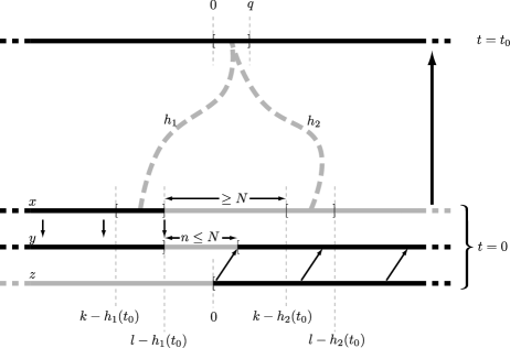
Figure 4: Construction of the configuration $y$ from a configuration $x$ and the periodic configuration $z$.

Moreover, $\llbracket k-h_{1}(t_{0}),l-h_{1}(t_{0})\rrbracket\subseteq\ \rrbracket-\infty,l-h_{1}(t_{0})\rrbracket$ and $\llbracket k-h_{2}(t_{0}),l-h_{2}(t_{0})\rrbracket\subseteq\llbracket l-h_{1}(t_{0})+n,+\infty\llbracket$, meaning that

$$F^{t_{0}}(x)_{\llbracket 0,q\rrbracket}=F^{t_{0}}(y)_{\llbracket 0,q\rrbracket}=F^{t_{0}}(\sigma^{m}(z))_{\llbracket 0,q\rrbracket}$$

where $m=-l+h_{1}(t_{0})-n$.

This shows that the factor $F^{t_{0}}(x)_{\llbracket 0,q\rrbracket}$ is in $\mathcal{L}_{\Sigma^{\prime}}$ (as a factor in the evolution of $\sigma^{m}(z)$). Because $F$ commutes with the shift, we have shown that all factors of size $q$ that appear after $t_{0}$ steps in the evolution of any configuration are in $\mathcal{L}_{\Sigma^{\prime}}$ and since $q$ is the order of $\Sigma^{\prime}$, it means that for all configuration $x$, $F^{t_{0}}(x)\in\Sigma^{\prime}$. Because $\Sigma^{\prime}$ is finite, the CA is nilpotent. ∎

The next proposition shows that in the case of a unique curve of equicontinuity (up to $\sim$), this curve is in fact equivalent to a rational slope.

Proposition 2.7.

Let $(\mathcal{A}^{\mathbb{Z}},F)$ be a CA and $\Sigma\subset\mathcal{A}^{\mathbb{Z}}$ a subshift. If there exists $h\in\mathcal{F}$ such that $\textbf{A}_{\mathbb{K}}^{\prime}(\Sigma,F)=\{h^{\prime}\in\mathcal{F}:h^{\prime}\sim h\}$, then there exists $\alpha\in\mathbb{Q}$ such that $h\sim h_{\alpha}$.

Proof.

Let $(\mathcal{A}^{\mathbb{Z}},F)$ be a non-nilpotent CA. By definition of $(\mathbb{N},\Sigma)$-equicontinuity along $h$, there exist $k,l\in\mathbb{Z}$, $k\leq l$, such that for all $x,x^{\prime}\in\Sigma$, if $x_{\llbracket k,l\rrbracket}=x^{\prime}_{\llbracket k,l\rrbracket}$ then for all $t\in\mathbb{N}$ one has:

$$F^{t}(x)_{h(t)}=F^{t}(x^{\prime})_{h(t)}$$

Thus the sequence $(F^{t}(x)_{h(t)})_{t\in\mathbb{N}}$ is uniquely determined by the knowledge of $x_{\llbracket k,l\rrbracket}$. For all $t\in\mathbb{N}$, consider the function

$$\begin{array}[]{rrcl}f_{t}:&\mathcal{L}_{\Sigma}(\llbracket k,l\rrbracket)&\longrightarrow&\mathcal{A}\\ &w&\longmapsto&F^{t}(x)_{h(t)}\textrm{ where }x\in[w]_{\llbracket k,l\rrbracket}\cap\Sigma\end{array}$$

Because there are finitely many functions from $\mathcal{L}_{\Sigma}(\llbracket k,l\rrbracket)$ to $\mathcal{A}$, there exist $t_{1},t_{2}\in\mathbb{N}$ such that $t_{1}<t_{2}$ and $f_{t_{1}}=f_{t_{2}}$.

For any configuration $x\in\Sigma$, and any cell $c\in\mathbb{Z}$,

$$F^{t_{1}}(x)_{h(t_{1})+c}=f_{t_{1}}(x\llbracket k+c,l+c\rrbracket)=f_{t_{2}}(x\llbracket k+c,l+c\rrbracket)=F^{t_{2}}(x)_{h(t_{2})+c}$$

We therefore have $F^{t_{1}}(x)=\sigma^{h(t_{2})-h(t_{1})}\circ F^{t_{2}}(x)$ for all possible configurations $x\in\Sigma$. With $\alpha=\frac{h(t_{2})-h(t_{1})}{t_{2}-t_{1}}$, $h_{\alpha}$ is a direction of equicontinuity of $(\mathcal{A}^{\mathbb{Z}},F)$. ∎

2.8 Properties of $\textbf{B}(\Sigma,F)$

The next proposition shows the link between expansivity and equicontinuous properties.

Proposition 2.8.

Assume $\mathbb{K}=\mathbb{N}$ or $\mathbb{Z}$. Let $(\mathcal{A}^{\mathbb{Z}},F)$ be a CA, $\Sigma$ be an infinite subshift. One has:

$$\left(\textbf{B}_{\mathbb{K}}^{r}(\Sigma,F)\cup\textbf{B}_{\mathbb{K}}^{l}(\Sigma,F)\right)\cap\textbf{A}_{\mathbb{K}}(\Sigma,F)=\emptyset.$$

In particular, if $\textbf{B}_{\mathbb{K}}(\Sigma,F)\neq\emptyset$ then $\textbf{A}_{\mathbb{K}}(\Sigma,F)=\emptyset$.

Proof.

Let $(\mathcal{A}^{\mathbb{Z}},F)$ be $(\mathbb{K},\Sigma)$-right expansive along $h$ with constant of expansivity $\varepsilon$. One has:

$$D^{h}_{\Sigma}(x,\varepsilon,\mathbb{K})\subset\{y\in\Sigma:y_{i}=x_{i}\ \forall i\geq 0\}.$$

Then the interior of $D^{h}_{\Sigma}(x,\varepsilon,\mathbb{K})$ is empty. Thus $Eq^{h}_{\mathbb{K}}(\Sigma,F)=\emptyset$.

Analogously, one proves $\textbf{B}_{\mathbb{K}}^{l}(\Sigma,F)\cap\textbf{A}_{\mathbb{K}}(\Sigma,F)=\emptyset$. In the case $\textbf{B}_{\mathbb{K}}(\Sigma,F)\neq\emptyset$, one has $\textbf{B}_{\mathbb{K}}^{r}(\Sigma,F)\cup\textbf{B}_{\mathbb{K}}^{l}(\Sigma,F)=\mathcal{F}$, so $\textbf{A}_{\mathbb{K}}(\Sigma,F)=\emptyset$. ∎

2.9 A dynamical classification along a curve

Theorem 2.9.

Let $(\mathcal{A}^{\mathbb{Z}},F)$ be a CA of neighborhood $\mathbb{U}=\llbracket r,s\rrbracket$. Let $\Sigma\subset\mathcal{A}^{\mathbb{Z}}$ be a weakly-specified subshift. Exactly one of the following cases hold:

1. $\textbf{A}_{\mathbb{N}}^{\prime}(\Sigma,F)=\textbf{A}_{\mathbb{N}}(\Sigma,F)=\mathcal{F}$. In this case $(\mathcal{A}^{\mathbb{Z}},F)$ is $\Sigma$-nilpotent, moreover $\textbf{B}_{\mathbb{N}}^{r}(\Sigma,F)=\textbf{B}_{\mathbb{N}}^{l}(\Sigma,F)=\emptyset$.

2. There exists $\alpha\in[-s,-r]\cap\mathbb{Q}$ such that $\textbf{A}_{\mathbb{N}}^{\prime}(\Sigma,F)=\textbf{A}_{\mathbb{N}}(\Sigma,F)=\{h:h\sim h_{\alpha}\}$. In this case there exist $m,p\in\mathbb{N}$ such that the sequence $(F^{n}\circ\sigma^{\lfloor\alpha n\rfloor})_{n\in\mathbb{N}}$ is ultimately periodic of preperiod $m$ and period $p$. Moreover, $\textbf{B}_{\mathbb{N}}^{l}(F^{m}(\Sigma),F)=]-\infty,\alpha[$ and $\textbf{B}^{r}(F^{m}(\Sigma),F)=]\alpha,+\infty[$.

3. There exist $h^{\prime},h^{\prime\prime}\in\mathcal{F}$, $h^{\prime}\prec h^{\prime\prime}$, $h^{\prime\prime}\precsim h_{-r}$ and $h_{-s}\precsim h^{\prime\prime}$ such that $\{h:h^{\prime}\prec h\prec h^{\prime\prime}\}\subset\textbf{A}_{\mathbb{N}}(\Sigma,F)\subset\{h:h^{\prime}\precsim h\precsim h^{\prime\prime}\}$. In this case $\textbf{A}_{\mathbb{N}}^{\prime}(\Sigma,F)=\textbf{B}_{\mathbb{N}}^{r}(\Sigma,F)=\textbf{B}_{\mathbb{N}}^{l}(\Sigma,F)=\emptyset$.

4. There exists $h^{\prime}\in\mathcal{F}$, $h_{-s}\precsim h^{\prime}\precsim h_{-r}$, such that $\textbf{A}_{\mathbb{N}}(\Sigma,F)=\{h:h\sim h^{\prime}\}$ and $\textbf{A}_{\mathbb{N}}^{\prime}(\Sigma,F)=\emptyset$. In this case $\textbf{B}_{\mathbb{N}}^{r}(\Sigma,F)$ and $\textbf{B}_{\mathbb{N}}^{l}(\Sigma,F)$ can be empty or not, but $\textbf{B}_{\mathbb{N}}(\Sigma,F)=\emptyset$.

5. $\textbf{A}_{\mathbb{N}}(\Sigma,F)=\textbf{A}_{\mathbb{K}}^{\prime}(\Sigma,F)=\emptyset$ but $\textbf{B}_{\mathbb{N}}(\Sigma,F)\not=\emptyset$.

6. $\textbf{A}_{\mathbb{N}}(\Sigma,F)=\textbf{A}_{\mathbb{N}}^{\prime}(\Sigma,F)=\textbf{B}_{\mathbb{N}}(\Sigma,F)=\emptyset$ but $\textbf{B}_{\mathbb{N}}^{r}(\Sigma,F)$ and $\textbf{B}_{\mathbb{N}}^{l}(\Sigma,F)$ can be empty or not.

Proof.

First, by proposition 2.6 and considering the possible values of $\textbf{A}_{\mathbb{N}}^{\prime}(\Sigma,F)$, we get a partition into: $C1$, $C2$, and $C^{\prime}=C3\cup C4\cup C5\cup C6$. The additional property in class $C2$ is obtained by proposition 2.7.

Then, inside $C^{\prime}$, the partition is obtained by discussing on $\textbf{A}_{\mathbb{N}}(\Sigma,F)$ (proposition 2.4) and $\textbf{B}_{\mathbb{N}}(\Sigma,F)$, non-emptyness of both being excluded by proposition 2.8. ∎

3 Equicontinuous dynamics: non-trivial constructions

This section aims at showing through non-trivial examples that the generalization of directional dynamics to arbitrary curve is pertinent.

3.1 Parabolas

Let us define the function

$$p:\left\{\begin{array}[]{rcl}\mathbb{N}&\rightarrow&\mathbb{Z}\\ x&\mapsto&\left\lfloor\frac{\sqrt{1+4(x+1)}-1}{2}\right\rfloor\end{array}\right.$$

whose inverse is

$$p^{-1}:\left\{\begin{array}[]{rcl}\mathbb{N}&\rightarrow&\mathbb{Z}\\ x&\mapsto&x(x+1)-1\end{array}\right.$$

This whole subsection will be devoted to the proof and discussion of the following result :

Proposition 3.1.

There exists a cellular automaton $(\mathcal{A}_{P}^{\mathbb{Z}},F_{P})$ such that

$$\textbf{A}_{\mathbb{N}}(\mathcal{A}_{P}^{\mathbb{Z}},F_{P})=\{h\in\mathcal{F}:p\precsim h\precsim\operatorname{id}\}$$

where $\operatorname{id}$ denotes the identity function $n\mapsto n$.

Proof.

Let us describe such an automaton. We will work on the standard neighborhood $\mathbb{U}_{P}=\{-1,0,1\}$ and use the set of 5 states $\mathcal{A}_{P}=\{\vbox to7.0pt{\hbox{\includegraphics{figures/dpst-1}}},\vbox to7.0pt{\hbox{\includegraphics{figures/dpst-3}}},\vbox to7.0pt{\hbox{\includegraphics{figures/dpst-4}}},\vbox to7.0pt{\hbox{\includegraphics{figures/dpst-2}}},\vbox to7.0pt{\hbox{\includegraphics{figures/dpst-5}}}\}$. The behavior of the automaton will be described in terms of signals : a cell in state should be seen as an empty cell with no signal, whereas all other states represent a given signal on the cell. There can only be one signal at a time on a given cell.

Signals move through the configuration. A signal can move to the left, to the right or stay on the cell it is (in which case we will say that the signal moves up because it makes a vertical line on the space-time diagram) as shown on Figure 5. A signal can also duplicate itself by going in two directions at a time (last case in figure 5).

Figure 5: Signals moving left (a), right (b), up (c) and both up and right (d).

We will now describe how each signal moves when it is alone (surrounded by empty cells) and how to deal with collisions, when two or more signals move towards the same cell (figure 6 provides a space-time diagram that illustrates most of these rules) :

• the signal moves up and right. It has priority over all signals except the one (signals with lesser priority disappear when a conflict arises) ;

• the signal moves up. It has priority over all signals except the aforementioned signal ;

• the signal moves left until it reaches a signal, at which point it becomes a signal (it turns around) instead of colliding into it ;

• finally, the signal moves right until it reaches a signal in which case it moves over it but turns into a signal (and therefore from there it moves away from the ). Not only the signal cannot go through a signal, as a consequence of what has been stated earlier, but it cannot cross a signal either (even if there was no real collision because the two could switch places) : it is erased by the signal moving in the opposite direction.

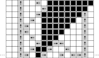
Figure 6: A space-time diagram of the described automaton on an example starting configuration.

The general behavior of the automaton can be described informally as follows:

• states form connex segments that expand towards the right and can be reduced from the left by signals ;

• signals create “vertical axes” on the space-time diagram ;

• and signals bounce back and forth from a vertical axis (on the left) to a segment (on the right). The border does not move but the on the right side is pushed to the right at each bounce ;

• signals can erase signals and by doing so “invade” a portion in which bouncing signals evolve. segments can merge when the right border of one reaches the left border of another.

We will now show that $\mathfrak{C}_{F_{P}}([\vbox to7.0pt{\hbox{\includegraphics{figures/dpst-5}}}]_{0})$, the set of consequences of the single-letter word $w=\vbox to7.0pt{\hbox{\includegraphics{figures/dpst-5}}}$ according to this automaton, is exactly the set of sites

$$\mathcal{P}_{0}=\{\langle c,t\rangle\ |\ t\geq 0,c\in\llbracket p(t),t\rrbracket\}$$

Fact 1:   $\mathcal{P}_{0}$ is exactly the set of sites in state in the space-time diagram starting from the initial finite configuration corresponding to the word (all other cells are in state ), as illustrated by Figure 7.

• Proof: It is clear from the behavior of the automaton that it takes $2(n+1)$ steps for the left border of the segment to move from cell $n$ to cell $(n+1)$. Conveniently enough, $p$ has the property that $p^{-1}(n+1)=p^{-1}(n)+2(n+1)$.

  $\Diamond$ Fact 1

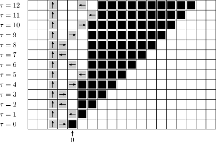
Figure 7: The set $\mathcal{P}_{0}$ is exactly the set of sites in state .

From Fact 3.1 we show that all sites that are not in $\mathcal{P}_{0}$ cannot be in the consequences of $w$ because if we start from the uniformly configuration (which is an extension of $w$) all states in the diagram are and hence these sites have different states depending on the extension of $w$ used as starting configuration.

Let us prove that conversely, for whatever starting configuration that contains $w$ at the origin, all sites in $\mathcal{P}_{0}$ are in state .

Fact 2:   If there exists a starting configuration $\mathcal{C}$ containing $w$ at the origin such that one of the sites $\langle c,t\rangle\in\mathcal{P}_{0}$ is in a state other than , then there exists a finite such starting configuration (one for which all cells but a finite number are in state ) for which the site $\langle c,t\rangle$ is in a state other than .

• Proof: The state in the site $\langle c,t\rangle$ only depends on the initial states of the cells in $\llbracket c-t,c+t\rrbracket$. The finite configuration that coincides with $\mathcal{C}$ on these cells and contains only states on all other cells has the announced property. $\Diamond$ Fact 2

The signal tends to propagate towards the top and the right. Since only the signal has priority over the one and because the former moves to the right, it cannot collide with the latter from the right side, which means that nothing can hinder the evolution of the signal to the right.

From now on, we will say that a connex segment of cells in state (that we will simply call a segment) is pushed whenever a signal bounces on its left border, and by doing so erases the leftmost state of the segment.

Fact 3:   Starting from an initial finite configuration, the time interval between two consecutive “pushes” of the leftmost state (by a signal) is exactly double the distance between it and the first state to its left, if any.

• Proof: All signals to the left of the leftmost segment are preserved. When a signal pushes the state, it generates a signal that moves left erasing all signals it meets on its way. Therefore nothing can reach the state while the signal is moving. When it reaches the first state (if there is one) and turns into a signal, the configuration is as follows :

  

  and nothing other than this newly produced signal will push the state. The time between the apparition of the signal after the first push until the push by the second signal is exactly double the distance between the and the states.

  Note. If there are no states to the left of the then there can be at most one push because the will never bounce back and will erase all signals before they reach the state. $\Diamond$ Fact 3

Fact 4:   If $c$ is the leftmost cell in state of a finite starting configuration, then all sites in $(\mathcal{P}_{0}+c)$ are in the state .

• Proof: From Fact 7 we show that the configuration corresponding to the word illustrates the fastest way to push a leftmost segment : it is the configuration where the signal is the closest possible to the (while still having a bouncing signal between them) and for which the first push happens at the earliest possible time.

  This means, in conjunction with Fact 3.1, that if $c$ is the leftmost cell originally in state then all sites in $(\mathcal{P}_{0}+c)$ are in state because its segment cannot be pushed faster. $\Diamond$ Fact 4

Fact 3.1 can be extended to all cells in state by induction :

Fact 5:   If a cell $c$ is in state in a finite starting configuration and that for all cells $c^{\prime}<c$ initially in state all sites in $(\mathcal{P}_{0}+c^{\prime})$ are in state , then all sites in $(\mathcal{P}_{0}+c)$ are in state .

• Proof: Let $c_{1}$ be the closest cell to the left of $c$ that is initially in state . Because the signal from $c_{1}$ propagates to the right at maximal speed, it can have no influence on the behavior of the segment generated by $c$ before it has actually reached it.

  This means that, until the two segments merge (at some time $t_{1}$), the segment from $c$ behaves as if it were the leftmost one, and therefore Fact 3.1 applies and ensures that all sites in

  $$\{\langle c,t\rangle\ |\ t<t_{1},c\in\llbracket c+p(t),c+t\rrbracket\}$$

  are in state .

  After the two segments merge, we know that all sites in

  $$\{\langle c,t\rangle\ |\ t\geq t_{1},c\in\llbracket c_{1}+p(t),c+t\rrbracket\}$$

  are in state . These include all remaining sites in $(\mathcal{P}_{0}+c)$ since $c_{1}<c$. $\Diamond$ Fact 5

By Fact 3.1, it is sufficient to show that for all finite extensions of $w$ all sites in $\mathcal{P}_{0}$ are in the state.

We then proceed by induction to show that for any cell $c$ in state on a finite initial configuration, all sites in $(\mathcal{P}_{0}+c)$ are in state (Fact 3.1 is the initialization, Fact 7 is the inductive step).

This concludes the proof that $\mathfrak{C}_{F_{P}}([\vbox to7.0pt{\hbox{\includegraphics{figures/dpst-5}}}]_{0})=\mathcal{P}_{0}$ and therefore

$$\{h\in\mathcal{F}:p\precsim h\precsim\operatorname{id}\}\subseteq\textbf{A}_{\mathbb{N}}(\mathcal{A}_{P}^{\mathbb{Z}},F_{P})$$

For the converse inclusion, let $h\in\textbf{A}_{\mathbb{N}}(\mathcal{A}_{P}^{\mathbb{Z}},F_{P})$ and suppose that $w$ is a blocking word along $h$. Then the word $vwv$ is also a blocking word along $h$ with $v=\vbox to7.0pt{\hbox{\includegraphics{figures/dpst-2}}}\vbox to7.0pt{\hbox{\includegraphics{figures/dpst-3}}}\vbox to7.0pt{\hbox{\includegraphics{figures/dpst-5}}}$. From the definition of $F_{P}$ we know that for any site $\langle z,t\rangle$ in the consequences of $vwv$, with $t\geq|vwv|$, and any configuration $x\in[vwv]_{0}$ then $F_{P}^{t}(x)_{z}=\vbox to7.0pt{\hbox{\includegraphics{figures/dpst-5}}}$ (because it is the case for the configuration everywhere in state except on the finite portion where it is $vwv$). Now, if we consider the sites in state generated by the configuration everywhere in state except on the finite portion where it is $vwv$, we have:

$$\langle z,t\rangle\in\mathfrak{C}_{F_{P}}([vwv]_{0})\Rightarrow\ p(t)+C_{1}\leq z\leq\operatorname{id}(t)+C_{2},$$

for some constants $C_{1}$ and $C_{2}$.

This completes the proof of Proposition 3.1. ∎

This shows that the notion of equicontinuous points following a non-linear curve is pertinent. This was an open question of [11].

An other open question of [11] was to find a cellular automaton such that $\widetilde{\textbf{A}}_{\mathbb{N}}(\mathcal{A}^{\mathbb{Z}},F)$ has open bounds.

Corollary 3.2.

There exists a CA $(\mathcal{A}^{\mathbb{Z}},F)$ such that $\widetilde{\textbf{A}}_{\mathbb{N}}(\mathcal{A}^{\mathbb{Z}},F)$ has open bounds.

Proof.

Choosing $F=F_{P}$, the result follows directly from Proposition 3.1: the set of slopes of straight lines lying between $p$ and $\operatorname{id}$ is exactly $]0,1]$. ∎

3.2 Counters

In this section we will describe a general technique that can be used to create sets of consequences that have complex shapes.

The general idea is to build the set of consequences in a “protected” area in a cone of the space-time diagram (the area between two signals moving in opposite directions) and making sure that nothing from the outside can affect the inside of the cone.

We will illustrate the technique on a specific example that will describe a CA for which the set of consequences of a single-letter word is the area between the vertical axis and a parabola. The counters construction will then also be used in section 4 to construct more complex sets of consequences.

Proposition 3.3.

There exists a cellular automaton $(\mathcal{A}^{\mathbb{Z}}_{C},F_{C})$ such that

$$\textbf{A}_{\mathbb{N}}(\mathcal{A}^{\mathbb{Z}}_{C},F_{C})=\{h\in\mathcal{F}:\monbb{0}\precsim h\precsim p\}$$

where $\monbb{0}$ denotes the constant fuction $n\mapsto 0$.

As in the previous section, we will show that the consequences of a single-letter word are exactly the set

$$\{\langle c,t\rangle\ |\ t\geq 0,c\in\llbracket 0,p(t)\rrbracket\}$$

3.2.1 General Description

The idea is to use a special state that can only appear in the initial configuration (no transition rule produces this state). This state will produce a cone in which the construction will take place. On both sides of the cone, there will be unary counters that count the “age of the cone”.

The counters act as protective walls to prevent external signals from affecting the construction. If a signal other than a counter arrives, it is destroyed. If two counters collide, they are compared and the youngest has priority (it erases the older one and what comes next). Because our construction was generated by a state on the initial configuration, no counter can be younger (all other counters were already present on the initial configuration).

The only special case is when two counters of the same age collide. In this case we can “merge” the two cones correctly because both contain similar parabolas (generated from an initial special state).

3.2.2 Constructing the Parabola inside the Cone

Inside the cone, we will construct a parabola by a technique that differs from the one explained in the previous section in that the construction signals are on the outer side.

The construction is illustrated by Figure 8. We see that we build two inter-dependent parabolas by having a signal bounce from one to the other. Whenever the signal reaches the left parabola, it drags it one cell to the right, and when it reaches the righ parabola it pushes it two cells to the right.

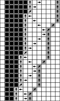
Figure 8: Construction of the parabola inside the cone.

It is easy to check that the left parabola advances as the one from the previous section : when it has advanced for the $n$-th time, the right parabola is at distance $n$ and therefore the signal will come back after $2n$ time steps.

The state (that will be the set of consequences, as in the previous section) moves up and right, but it is stopped by the states of the left parabola.

3.2.3 The Younger, the Better

The state produces 4 distinct signals. Two of them move towards the left at speed $1/4$ and $1/5$ respectively. The other two move symmetrically to the right at speed $1/4$ and $1/5$.

Each couple of signals (moving in the same direction) can be seen as a unary counter where the value is encoded in the distance between the two. As time goes the signals move apart.

Note that signals moving in the same direction (a fast one and a slow one) are not allowed to cross. If such a collision happens, the faster signal is erased. A collision cannot happen between signals generated from a single state but could happen with signals that were already present on the initial configuration. Collisions between counters moving in opposite directions will be explained later as their careful handling is the key to our construction.

Because the state cannot appear elsewhere than the initial configuration and counter signals can only be generated by the state (or be already present on the initial configuration), a counter generated by a state is at all times the smaller possible one: no two counter signals can be closer than those that were generated together. Using this property, we can encapsulate our construction between the smallest possible counters. We will therefore be able to protect it from external perturbations: if something that is not encapsulated between counters collides with a counter, it is erased. And when two counters collide we will give priority to the youngest one.

3.2.4 Dealing with collisions

Collisions of signals are handled in the following way:

• nothing other than an outer signal can go through another outer signal (in particular, no “naked information” not contained between counters);

• when two outer signals collide they move through each other and comparison signals are generated as illustrated by Figure 9;

• on each side, a signal moves at maximal speed towards the inner border of the counter, bounces on it ($C$ and $C^{\prime}$) and goes back to the point of collision ($D$);

• The first signal to come back is the one from the youngest counter and it then moves back to the outer side of the oldest counter ($E$) and deletes it;

• the comparison signal from the older counter that arrives afterwards ($D^{\prime}$) is deleted and will not delete the younger counter’s outer border;

• all of the comparison signals delete all information that they encounter other than the two types of borders of counters.

Figure 9: The bouncing signal must arrive (point $E$) before the older counter moves through the younger one (point $F$).

Counter Speeds

It is important to ensure that the older counter’s outer border is deleted before it crosses the younger’s inner border. This depends on the speeds $s_{o}$ and $s_{i}$ of the outer and inner borders. It is true whenever $s_{o}\leq\frac{1-s_{i}}{s_{i}+3}$. If the maximal speed is $1$ (neighborhood of radius $1$), it can only be satisfied if

$$s_{i}<\sqrt{5}-2\simeq 0.2360$$

This means that with a neighborhood of radius 1 the inner border of the counter cannot move at a speed greater than $(\sqrt{5}-2)$. Any rational value lower than this is acceptable. For simplicity reasons we will consider $1/5$ (and the corresponding $1/4$ for the outer border of the counter). If we use a neighborhood of radius $k$, the counter speeds can be increased to $k/5$ and $k/4$.

Exact Location

Note that a precise comparison of the counters is a bit more complex than what has just been described. Because we are working on a discrete space, a signal moving at a speed less than maximal does not actually move at each step. Instead it stays on one cell for a few steps before advancing, but this requires multiple states.

In such a case, the cell on which the signal is is not the only significant information. We also need to consider the current state of the signal: for a signal moving at speed $1/n$, each of the $n$ states represents an advancement of $1/n$, meaning that if a signal is located on a cell $c$, depending on the current state we would consider it to be exactly at the position $c$, or $(c+1/n)$, or $(c+2/n)$, etc. By doing so we can have signals at rational non-integer positions, and hence consider that the signal really moves at each step.

When comparing counters, we will therefore have to remember both states of the faster signals that collide (this information is carried by the vertical signal) and the exact state in which the slower signal was when the maximal-speed signal bounced on it. That way we are able to precisely compare two counters: equality occurs only when both counters are exactly synchronized.

The Almost Impregnable Fortress

Let us now consider a cone that was produced from the state on the initial configuration. As it was said earlier, no counter can be younger than the ones on each side of this cone. There might be other counters of exactly the same age, but then these were also produced from a state and we will consider this case later and show that it is not a problem for our construction.

Nothing can enter this cone if it is not preceded by an outer border of a counter. If an opposite outer border collides with our considered cone, comparison signals are generated. Because comparison signals erase all information but the counter borders, we know that the comparison will be performed correctly and we do not need to worry about interfering states. Since the borders of the cone are the youngest possible signals, the comparison will make them survive and the other counter will be deleted.

Note that two consecutive opposite outer borders, without any inner border in between, are not a problem. The comparison is performed in the same way. Because the comparison signals cannot distinguish between two collision points (the vertical signal from $O$ to $D$ in Figure 9) they will bounce on the first they encounter. This means that if two consecutive outer borders collide with our cone, the comparisons will be made “incorrectly” but this error will favor the well formed counter (the one that has an outer and an inner border) so it is not a problem to us.

Evil Twins

The last case we have to consider now is that of a collision between two counters of exactly the same age. Because the only counter that matters to us is the one produced from the state (the one that will construct the parabola), the case we have to consider is the one where two cones produced from a state on the initial configuration collide. These two cones contain similar parabolas in their interior.

According to the rules that were described earlier, both colliding counters are deleted. This means that the right side of the leftmost cone and the left part of the rightmost cone are now “unprotected” and facing each other. From there, the construction of the two parabolas will merge, as illustrated in Figure 10.

Figure 10: Two “twin” parabolas merging.

The key point here is the fact that the two merged parabolas were “parallel” meaning that the one on the left would never have passed beyond the one on the right. Because of this, for as long as the rightmost parabola is constructed correctly, all states that should have been because of the construction of the left parabola will be .

3.2.5 The Transparency Trick

We have shown that all sites that would be in the evolution of a “lonely” state (all other initial cells being in the blank state) will stay in the state no matter what is on the other cells of the initial configuration. Now we have to show that no other sites than these are in the consequences of the state.

To do so, we will use a very simple trick. We consider our automaton as it was described so far, and add a binary layer with states $0$ and $1$. This layer is free and independent of the main layer, except if the state on the main layer is in which case the binary layer state can only be $0$. More precisely, this layer is kept unchanged except when entering into state on the main layer in which case it becomes $0$. Let’s call $F_{C}$ the final CA obtained.

Now, if we consider configurations where the main layer is made of a single state on a blank configuration, we are guaranteed that states cannot disappear once present in a cell. Hence, at any time, any cell not holding the state contains the value from the initial configuration in this additional layer. This means that, for such initial configurations, all sites can be changed except those holding state . This means that the consequences of the single-letter word $(\vbox to7.0pt{\hbox{\includegraphics{figures/dpst-11}}},0)$ (this is a single state in the two-layered automaton) are exactly

$$\mathfrak{C}_{F_{C}}([(\vbox to7.0pt{\hbox{\includegraphics{figures/dpst-11}}},0)]_{0})=\{\langle c,t\rangle\ |\ t\geq 0,c\in\llbracket 0,p(t)\rrbracket\}$$

This concludes the proof of Proposition 3.3.

The counters construction used to protect the evolution of the parabola gives $F_{C}$ a special property: all equicontinuous points are Garden-of-Eden configurations. To our knowledge, this is the first constructed CA with this property.

Corollary 3.4.

There exists a CA $(\mathcal{A}^{\mathbb{Z}},F)$ having (classical) equicontinuous points, but all being Garden-of-Eden configurations (i.e. configurations without a predecessor).

Proof.

We choose $F=F_{C}$. The corollary follows from the fact that any blocking word must contain the state . To see this suppose that some blocking word $w$ do not contain the state . Then, whatever $w$ is, it cannot produce a protective cone as “young” as the one generated by . Therefore, if $c\in[w]_{0}$ contains the state somewhere, the outer signal generated by will reach the central cell at some time depending on the position of the first occurrence of in $c$, and, after some additional time, the central cell will become and stay in this state forever. This way, we can choose two configurations $c,c^{\prime}\in[w]_{0}$ such that the sequence of states taken by the central cell are different: this is in contradiction with $w$ being a blocking word. ∎

By combining the two constructions from Propositions 3.1 and 3.3 we can obtain a CA with only one direction (up to $\sim$) along which the CA has equicontinuity points and such that this direction is not linear. This is another example where the generalization of directional dynamics to arbitrary curves is meaningful.

Corollary 3.5.

There exists a CA $(\mathcal{A}^{\mathbb{Z}},F)$ with $\textbf{A}_{\mathbb{N}}(\mathcal{A}^{\mathbb{Z}},F)=\{h:h\sim h_{0}\}$ where $h_{0}$ is not linear.

Proof.

It is straightforward that for any pair of CA $G,H$ we have:

$$\textbf{A}_{\mathbb{N}}(\mathcal{A}^{\mathbb{Z}}_{G}\times\mathcal{A}^{\mathbb{Z}}_{H},G\times H)=\textbf{A}_{\mathbb{N}}(\mathcal{A}^{\mathbb{Z}}_{G},G)\cap\textbf{A}_{\mathbb{N}}(\mathcal{A}^{\mathbb{Z}}_{H},H)$$

Let $F=F_{P}\times F_{C}$. By propositions 3.1 and 3.3, $\textbf{A}_{\mathbb{N}}(\mathcal{A}_{P}^{\mathbb{Z}}\times\mathcal{A}^{\mathbb{Z}}_{C},F)=\{h:h\sim p\}$. ∎

4 Equicontinuous dynamics along linear directions

By a result from [11], we know that the set of slopes of linear directions along which a CA has equicontinuous points is an interval of real numbers. In this section we are going to study precisely the possible bounds of such intervals.

4.1 Countably enumerable numbers

Definition 4.1.

A real number $\alpha$ is countably enumerable (ce) if there exists a computable sequence of rationals converging to $\alpha$.

The previous definition can be further refined as follows:

Definition 4.2.

A real number $\alpha$ is left (resp. right) countably enumerable (lce) (resp. rce) if there exists an increasing (resp. decreasing) computable sequence of rationals converging to $\alpha$.

Remark 4.1.

A real number that is both lce and rce is computable.

See [14] for more details.

In the following we first prove that the bounds of the interval of slopes of linear directions along which a CA has equicontinuous points are computably enumerable real numbers. We will then give a generic method to construct a CA having arbitrary computably enumerable numbers as bounds for the slopes along which it has equicontinuity points.

4.2 Linear directions in the consequences of a word

We consider in this section computable subshifts only, that is subshifts for which we can decide whether or not a given word belongs to it (in particular, all finite type and sofic subshifts are decidable). For a word $u\in\Sigma$ and a CA $(\mathcal{A}^{\mathbb{Z}},F)$, we note

$$I_{u}=\{\alpha\in\mathbb{R}\ |\ u\ is\ a\ blocking\ word\ of\ slope\ h_{\alpha}\ for\ F\}.$$

$I_{u}$ is an interval and we note it $|a_{u},b_{u}|$. The bounds can either be open or closed. We will show that this bounds are lce (resp. rce).

The proof uses the notion of blocking word along $h$ during a time $T$, which intuitively is a word that doesn’t let information go through its consequences before time $(T+1)$. The definition can be adapted from definition 2.3 by replacing $\mathbb{K}$ by $\llbracket 0,T\rrbracket$, formally:

$$\mathfrak{C}_{F}(\Sigma\cap[u]_{p})\supset\left\{\langle m,n\rangle\in\mathbb{Z}\times\llbracket 0,T\rrbracket:h(n)\leq m<h(n)+e\right\}.$$

Notice that if some word is blocking of slope $h$ during arbitrary long time, it is clearly $\mathbb{N}$-blocking of slope $h$ too.

If time $T$ is fixed, the set of slopes for which a word $u$ is blocking during time $T$ is a convex set. This is formalized by the following Lemma which is a weakened version of Proposition 2.4.

Lemma 4.1.

Let $F$, $u$, $T$ and $\alpha<\beta$ be such that $u$ is a blocking word for $F$ along $h_{\alpha}$ (resp. $h_{\beta}$) during time $T$. Then, for any $\gamma\in[\alpha,\beta]$, $u$ is also a blocking word along $h_{\gamma}$ during time $T$.

Proof.

Straightforward. ∎

Proposition 4.2.

Let $\Sigma$ be a computable subshift and $(\mathcal{A}^{\mathbb{Z}},F)$ a CA. For $u\in\Sigma$, with $I_{u}=|a_{u},b_{u}|$, $a_{u}$ is lce and $b_{u}$ is rce.

Proof.

We consider configurations in which $u$ is placed on the origin. For every $n\in\mathbb{N}$, the set of cells in the consequences of $u$ at time $n$ is computable since only a finite number of factors on finitely many configurations have to be considered (the factors can be computed because the subshift is computable).

Consider $x_{n}$ the smallest integer such that $u$ is a blocking word during time $n$ of slope $h_{\frac{x_{n}}{n}}$. The sequence defined by $\alpha_{1}=x_{1}$ and $\alpha_{n+1}=max\left(\frac{x_{n+1}}{n+1},\alpha_{n}\right)$ is increasing and clearly computable from what was said above.

Now let $a\in I_{u}$. Because $u$ is a blocking word of slope $a$, it is also a blocking word of slope $a$ during time $n$, which means that $\forall n\in\mathbb{N},\frac{x_{n}}{n}\leq a$, so $\forall n\in\mathbb{N},\alpha_{n}\leq a$. Therefore, the sequence $(\alpha_{n})_{n}$ tends toward some limit $\alpha\leq a$. As it is true for any $a\in I_{u}$, we have $\alpha\leq a_{u}$. Suppose for the sake of contradiction that there is some $b$ with $\alpha\leq b<a_{u}$. Then, by Lemma 4.1, $b^{\prime}=\frac{a_{u}+b}{2}$ is such that $u$ is a blocking word of slope $b^{\prime}$ for arbitrary long time (because $\alpha$ and any $a\geq a_{u}$ are), hence a $\mathbb{N}$-blocking word of slope $b^{\prime}$. We get $b^{\prime}\in I_{u}$ which is a contradiction since $b^{\prime}<a_{u}$. Thus $a_{u}\leq\alpha$ and finally $a_{u}=\alpha$. We deduce that $a_{u}$ is lce.

A symmetric proof shows that $b_{u}$ is rce. In fact the situation is not formally symmetric since we consider functions of the form $h_{\alpha}(n)=\lfloor\alpha n\rfloor$. However it is obvious that $h^{\prime}_{\alpha}(n)=\lceil\alpha n\rceil$ is such that $h_{\alpha}\sim h^{\prime}_{\alpha}$. Then Proposition 2.3 allows to make a symmetric reasonning on functions of the form $h^{\prime}_{\alpha}$ and still have a conclusion for function of the form $h_{\alpha}$ which are considered in the statement of the current Proposition. ∎

In the proof above, we actually showed that $a_{u}$ and $b_{u}$ were directions of equicontinuity. So the set of linear directions of equicontinuity is closed for a word.

4.3 Bounds for $\widetilde{\textbf{A}}_{\mathbb{K}}(\Sigma,F)$

Theorem 4.3.

Let $\Sigma$ be a computable subshift and $(\mathcal{A}^{\mathbb{Z}},F)$ a CA. Let $\widetilde{\textbf{A}}_{\mathbb{K}}(\Sigma,F)=\{h_{\alpha}:\alpha\in|\alpha^{\prime},\alpha^{\prime\prime}|\}$.

Both $\alpha^{\prime}$ and $\alpha^{\prime\prime}$ are ce. Moreover, if $|\alpha^{\prime},\alpha^{\prime\prime}|$ is left-closed, $\alpha^{\prime}$ is lce, and if $|\alpha^{\prime},\alpha^{\prime\prime}|$ is right-closed then $\alpha^{\prime\prime}$ is rce.

Proof.

We prove it for left bounds, the proofs are similar for right bounds. There are two cases: the interval is either left-closed or left-open. The first case follows from Proposition 4.2 since there exists a word $u$ such that the left bound of slopes of $\widetilde{\textbf{A}}_{\mathbb{K}}(\Sigma,F)$ is the left bound of $I_{u}$.

In the case of an open bound, we produce a sequence converging to it. Suppose $\widetilde{\textbf{A}}_{\mathbb{K}}(\Sigma,F)=]\alpha^{\prime},\alpha^{\prime\prime}|$, then for every $i\in\mathbb{N}$, there exist $u_{i}$ such that $I_{u_{i}}=|x_{i},y_{i}|$ with $x_{i}\in]\alpha^{\prime},\alpha^{\prime}+1/i]$. So these $x_{i}$ are lce and the sequence $(x_{i})_{i}$ tends to $\alpha^{\prime}$. For every $i\in\mathbb{N}$ let $(y_{i,k})_{k}$ be a rational sequence converging to $x_{i}$. $(y_{i,i})_{i}$ is a rational sequence converging to $\alpha^{\prime}$, hence $\alpha^{\prime}$ is ce. ∎

Here, we consider linear directions of equicontinuity for a CA, so the intervals of admissible directions can be open or closed.

In the case when there is a single linear equicontinuous direction, we have the following corollary:

Corollary 4.4.

For $\Sigma$ a computable subshift and a CA $(\mathcal{A}^{\mathbb{Z}},F)$, if there exists $\alpha\in\mathbb{R}$ such that $\widetilde{\textbf{A}}_{\mathbb{K}}(\Sigma,F)=\{h_{\alpha}\}$ then $\alpha$ is computable.

Proof.

As $\alpha$ is both a closed left and a closed right bound, it is left and right computably enumerable so it is computable. ∎

4.4 Reachability

We prove here that any computably enumerable number is realized as a bound for $\{\alpha|h_{\alpha}\in\widetilde{\textbf{A}}_{\mathbb{K}}(\mathcal{A}^{\mathbb{Z}},F)\}$ on some cellular automaton $F$. The idea of the construction is to use the counters described in Subsection 3.2 combined with methods to obtain signals of computably enumerable slopes.

We will prove the following result:

Proposition 4.5.

For every ce number $0\leq\alpha\leq 1$, there exists a CA $(\mathcal{A}^{\mathbb{Z}},F)$ and a word $u\in\mathcal{A}^{*}$ such that $I_{u}=]\alpha,1]$.

The idea consists in constructing an area of states (which will be the desired set of consequences) limited to the right by a line of slope 1, and to the left by a curve that tends to the line of slope $\alpha$. As in the construction of the parabola from Subsection 3.1, the signal will move up and right, and a specific signal will be able to turn a state into a state. We will then send the correct density of signals to get the right slope.

As $\alpha$ is ce, there exists a Turing machine that enumerates a sequence of rationals $(\alpha_{i})_{i\in\mathbb{N}}$ that tends to $\alpha$.

One cell initializes the whole construction. It creates the area and starts a Turing machine on its left. This machine has to perform several tasks.

4.4.1 Sending signals

First it creates successive columns of size $2^{i},\ i\in\mathbb{N}$. Columns are delimited by a special state and contain blank states. In each column, a signal bouces back and forth from one border to the other. The time needed to go from the right border of the column to the left border and back again to the right border is $2^{i+1}$ (see Figure 11).

The right border of a column can be either active ( state) or resting ( state). If a column is activated, it will send a signal to the right each time the bouncing signal reaches it (i.e. every $2^{i+1}$ steps). This signal, when emitted, passes through all other columns and continues until it reaches a state. The state is erased (therefore pushing the border of the surface one cell to the right) and the signal disappears. If a column is resting, no signal is emitted when the bouncing signal hits the right border.

The Turing machine constructs and initializes the columns in order to synchronize the internal signals: the signal in column $(i+1)$ hits the right border at a time when the one in column $i$ hits its right border, as shown in Figure 11 (this is possible because the period of each signal is exactly double the period of the previous signal). When a signal is emitted by column $i$, it has to move through all the previous columns. Because the columns are synchronized, it will pass through the column $0$ at time $(n\times 2^{i+1}+2^{i}-1)$ for some $n$. This means that two signals emitted by different columns cannot be on the same diagonal (in the space-time diagram) and therefore cannot collide.

For every $i\in\mathbb{N}$, when the $i$ first columns are all created, the machine computes $\alpha_{i}$ with precision $2^{-(i+1)}$. The machine then activates only the columns $k\leq i$ such that the $k$-th bit of $\alpha_{i}$ is $1$. At that time the density of signals emitted by the columns is in $[\alpha_{i}-2^{-(i+1)},\alpha_{i}+2^{-(i+1)}]$.

Moreover, as the sequence $(\alpha_{i})_{i}$ converges to $\alpha$, for any $j\in\mathbb{N}$ there exists $i_{j}$ such that: $\forall i\geq i_{j}$, $\alpha$ and $\alpha_{i}$ share their $j$ first bits. And at some time, the Turing machine computes $\alpha_{i_{j}}$. From then on, the $j$ first columns are in their final state since they represent the $j$ first bits of $\alpha_{i}$, $i\geq i_{j}$. So the process converges and as these bits are the $j$ first bits of $\alpha$ too, the constructed slope tends to the desired one.

Figure 11: Columns and signals. Here the columns of width 2, 4 and 16 are active and the signals that go through them push the black area at regular intervals.

4.4.2 Density of signals

We here name density, the average number of signals emitted by a line or reaching a line during a timestep. Because $(\alpha_{i})_{i}$ tends to $\alpha$, each column will be in a permanent state (active or resting) after a long enough time. The density of signals emitted (passing through a vertical line) by the columns will tend to $\alpha$ as time passes. However, because signals have to reach a line that is not vertical (the border of the surface), the density of signals effectively reaching this line is less (a kind of Doppler effect). If we want to get a line of slope $\alpha$, $\alpha$ signals should reach the frontier at each timestep. As shown in Figure 12, if the density of emitted signals is some $\beta$, we have $\beta(1-\alpha)$ signals reaching the frontier, so we want $\beta(1-\alpha)=\alpha$. And finally, we need to emit signals with a density equal to $\frac{\alpha}{1-\alpha}$. Clearly, as $\alpha$ is ce, $\frac{\alpha}{1-\alpha}$ is ce too so it is possible to emit the correct density of signals.

Figure 12: Signals approaching at speed 1 reach the frontier with a lesser density.

4.4.3 Equicontinuity

If only the state can move through the borders of the columns (and by doing so destroys them) the consequences of the initializing cell are an area containing lines of slopes between $\alpha$ and $1$. We use again the transparency trick described in 3.2.5. The left bound ($\alpha$) is not necessarily closed. If $\alpha$ is lce, we have an increasing sequence converging to it and so the slope of the curve bounding the area on the left is lower than $\alpha$. So if $\alpha$ is lce, we can make a construction such that the bound is closed.

4.4.4 Right side

It is possible to do a symmetric construction on the other side. We can then have an area of states between the line of slope $-1$ and the line of slope $\alpha$. The construction must however be slightly modified.

If we consider an automaton with a larger radius, we can have “diagonal columns” delimited by lines of slope 1. In this case, the signals emitted by the columns move towards the left and they “pull” the black area instead of pushing it (in a way that is very similar to the construction of the parabola in Subsection 3.2). If we “protect” this construction between counters as seen in Subsection 3.2 it becomes a set of consequences.

4.4.5 Results

With the previous constructions and cartesian products if necessary, we have a sort of converse of Theorem 4.3:

Theorem 4.6.

Let $\alpha^{\prime}\leq\alpha^{\prime\prime}$ be ce real numbers. There exists a CA $(\mathcal{A}^{\mathbb{Z}},F)$ such that $\widetilde{\textbf{A}}_{\mathbb{K}}(\mathcal{A}^{\mathbb{Z}},F)=|\alpha^{\prime},\alpha^{\prime\prime}|$. Moreover, if $\alpha^{\prime}$ is lce the left bound can be closed: $\widetilde{\textbf{A}}_{\mathbb{K}}(\mathcal{A}^{\mathbb{Z}},F)=[\alpha^{\prime},\alpha^{\prime\prime}|$. If $\alpha^{\prime\prime}$ is rce, the right bound can be closed.

We use the CA constructed in 4.5. For each set of directions, we had a word $u$ with exactly the desired set of consequences. It remains to prove that there is no other linear direction of equicontinuity. This can be achieved by considering a blocking word $v$ along another linear direction, and using the same kind of arguments as in 3.1. Then $uvu$ brings a contradiction since the consequences of $v$ should extend outside the consequences of one of the $u$. Which is not possible since $u$ is blocking.

5 Equicontinuous dynamics: constraints and negative results

This section aims at showing that some sets cannot be consequences of any word on a cellular automaton. We know that the consequences of a word $u$ cannot extend to cells that never receive any information from $u$ (except for nilpotent CA). But there are other constraints, and we study them here. For example, a natural idea is to put a word $u$, 2 or more times on the initial configuration. Thus, the space-time diagram contains the consequences of $u$ and a copy of them spatially translated. Clearly, the sites in the intersection of the consequences with its copy’s have one unique state and so, we can get relations between the states of different sites of the consequences. In this part we give some conditions on a set of sites to be a potential set of consequences.

5.1 States in a set of consequences

Let $F$ be a CA, $u$ be a word and $n\geq|u|\in\mathbb{N}$. First, we consider configurations $c\in\mathcal{A}^{\mathbb{Z}}$ containing a second occurrence of $u$ translated of $n$ cells on the right, i.e. $\exists n\geq|u|$, ${c\in[u]_{0}}$ and ${\sigma^{n}(c)\in[u]_{0}}$. We denote by $\mathcal{C}(u)$ the set of consequences $\mathfrak{C}_{F}([u]_{0})$. Now, suppose there exist two sites $\langle x,t\rangle$ and $\langle x+n,t\rangle$ in $\mathcal{C}(u)$, for $x\in\mathbb{Z}$ and $t\in\mathbb{N}$. If the site $\langle x,t\rangle$ is in the state $a\in\mathcal{A}$, then, considering the translation of $\mathcal{C}(u)$, the site $\langle x+n,t\rangle$ is in the state $a$. So the consequences $\mathcal{C}(u)$ impose that the sites $\langle x,t\rangle$ and $\langle x+n,t\rangle$ are in the same state. The following proposition generalizes this simple idea.

Proposition 5.1.

If, for some $l\in\mathbb{N}$, the set of consequences of a word $u\in\mathcal{A}^{l}$ contains the sites $\langle x,t\rangle$ and $\langle x+2l,t\rangle$ for some $x\in\mathbb{Z}$ and $t\in\mathbb{N}$, then all the sites $\langle y,t\rangle$ ($y\in\mathbb{Z}$) such that $\langle y,t\rangle\in\mathcal{C}(u)$, are in the same state for any initial configuration of $[u]_{0}$.

Proof.

For any $y\in\mathbb{Z}$, either $|y-x|\geq l=|u|$, or $|y-(x+2l)|\geq l=|u|$. So considering what was proved just above, $\langle y,t\rangle$ is in the same state as either $\langle x,t\rangle$ or $\langle x+2l,t\rangle$. And the same argument proves that these both sites share their state too. ∎

5.2 Constraints coming from periodic initial configurations

For $n\in\mathbb{N}$ and $u\in\mathcal{A}^{n}$, we now consider initial configurations that are periodic of period $uv$ for some $v$. We use the fact that they lead to an ultimately periodic space-time diagram. First we consider $v$ of length $0$, we then have $u^{\mathbb{Z}}$ for initial configuration. We have a ultimately periodic diagram, and so, we can tell that the states of the consequences follow a ultimately periodic pattern. The following lemma illustrates a particular case where we can show that the consequences of a word $u$ are eventually spatially uniform: all sites in the consequences of $u$ at any given large enough time are in the same state.

Lemma 5.2.

Suppose that for some word $u$ of length $n$, all the space-time diagrams with initial configurations in $S=\{(uv)^{\mathbb{Z}}:|v|=n^{2}\}$ have identical periodic part. Then the consequences of $u$ are eventually spatially uniform.

Proof.

Consider periodic configurations of the form $(uv)^{\mathbb{Z}}$ with $v=u^{n}$ and $v=a(ua)^{n-1}$ ($a\in\mathcal{A}$), respectively. They respectively have (spatial) period lengths $|u|$ and $|u|+1$, so their space-time diagrams too. Since they are in $S$, the equality of their periodic part implies that they have both spatial periods $|u|$ and $|u|+1$. It follows that it has period $1$, so the periodic part is eventually spatially uniform, and in particular, the consequences of $u$ are eventually spatially uniform. ∎

We will study below examples of sets of consequences where the lemma applies. As we want to show the equality of two periodic space-time diagrams, we only need to show it on one spatial period at some time. So we will only show the equality of both configurations on a segment of length $n^{2}+n$.

We denote by $P_{uv}$ and $P_{uw}$ the space-time diagrams with periodic initial configurations of periods $uv$ and $uw$ ($|v|=|w|=n^{2}$). In the periodic part of them, the spatial period will be $n^{2}+n$, and the temporal periods will be $T_{uv}$ and $T_{uw}$. So, a common period can be defined by vectors $(n^{2}+n,0)$ and $(0,T)$ where $T=T_{uv}T_{uw}$.

5.2.1 Parabola

We now consider a word $u$ whose set of consequences draws a discrete parabola. The definition of a parabola that we will use here is that it is a sequence of vertical segments of increasing lengths, and translated by 1 to the right compared to the previous one. More formally, we suppose that the set of consequences of $u$ verifies the following:

$$\mathcal{C}(u)\supset\left\{\langle x,y\rangle:f(x)\leq y<f(x+1)\right\},$$

for some polynomial function $f$ which is strictly increasing on $\mathbb{N}$, and such that ${x\mapsto f(x+1)-f(x)}$ is strictly increasing too.

Proposition 5.3.

If the consequences of some word $u$ contains a parabola in the above sense then they are eventually spatially uniform.

Proof.

Let’s suppose $T_{0}$ is the smallest integer such that after $T_{0}$, both $P_{uv}$ and $P_{uw}$ are in their periodic part. Now we take $x^{\prime}$ such that $T\leq f(x^{\prime}+1)-f(x^{\prime})$. We take $t>T_{0}$ and $x>x^{\prime}$ such that $\langle x,t\rangle\in\mathcal{C}(u)$. These $x$ and $t$ exist thanks to the definition of $\mathcal{C}(u)$, and they are large enough to be in the periodic part of both diagrams.

We now show that $P_{uv}$ and $P_{uw}$ coincide on the sites $\langle x+k,t\rangle$ for $0\leq k<n^{2}+n$ and lemma 5.2 concludes. To do this we show that, for any $k$, there exists a site $s\in\mathcal{C}(u)$ such that

$$P_{uv}(\langle x+k,t\rangle)=P_{uv}(s)=P_{uw}(s)=P_{uw}(\langle x+k,t\rangle).$$

To find this site $s$, we consider the temporal periodicity: at $t+mT$, the states will be the same as at $t$ in $P_{uv}$ (period $T_{uv}$) and in $P_{uw}$ (period $T_{uw}$) for all $m$. From that, it is sufficient to find for each $1\leq k<n^{2}+n$ an $m$ such that $s=\langle x+k,t+mT\rangle\in\mathcal{C}(u)$. As we have taken $x>x^{\prime}$ and with the properties of $f$, we know that $f(x+k+1)-f(x+k)\geq T$ and there are more than $T$ consecutive sites of abscissa $x+k$ in $\mathcal{C}(u)$, so such an $m$ exists for all $k$. ∎

The proposition applies to the examples constructed in the previous section. It shows that the non-linear set of consequences like parabolas are obtained at the price of spacial uniformity.

5.2.2 Non-periodic walls

Now we consider a wall $u$ along some $h$ (with bounded variations) where $\forall\alpha\in\mathbb{Q},h\nsim h_{\alpha}$. In this case again, the consequences of $u$ are eventually spatially uniform.

Proposition 5.4.

If there exists a blocking word $u$ along $h$ such that $\forall\alpha\in\mathbb{Q},h\nsim h_{\alpha}$, then the consequences of $u$ are eventually spatially uniform.

Proof.

We once more consider the set of configurations $\{(uv)^{\mathbb{Z}}:|v|=|u|^{2}\}$, and prove that the periodic parts of the generated space-time diagrams are all identical. Then lemma 5.2 concludes. Let $v$ and $w$ be arbitrary words of length $|u|^{2}$. If some site $\langle x,t\rangle$ has different states in the space-time diagrams $P_{uv}$ and $P_{uw}$, there must be another site $\langle y,t-1\rangle$ with different states too. And $x-y$ must be bounded by the radius of the automaton. So if there are differences in the periodic parts of $P_{uv}$ and $P_{uw}$, we have a sequence of sites $s_{n}=\langle x_{n},n\rangle$ with different states in both diagrams. And for all $n>0$, $x_{n}-x_{n-1}$ is bounded by the radius of the automaton, but a wall is by definition larger than the radius of the automaton, so this sequence can’t cross a wall. Since the set of sites where $P_{uv}$ and $P_{uw}$ differ is periodic after some time, the sequence $(s_{n})$ can also be chosen ultimately periodic. So we have a sequence that can’t cross a wall either, and that is ultimately periodic. But we can have the same sequence translated on the other side of the wall. So the wall is between two sequences with the same (ultimate) period. We can associate a slope $\alpha$ to this period, and thus we have $h\sim h_{\alpha}$ for some $\alpha\in\mathbb{Q}$. Which is a contradiction. ∎

5.3 Reversible CA

We now restrict to reversible CA. Arguments developed earlier have stronger consequences in this case.

Proposition 5.5.

On a reversible CA, if the set of consequences of a word $u$ of length $n$ contains all sites $\langle x+k,t\rangle$ for $0\leq k\leq 2n-1$ and some $x$ and $t$, then $u$ is uniform and $\mathcal{C}(u)$ are eventually spatially uniform.

Proof.

Proposition 5.1 let us conclude that a long segment of sites in the consequences of $u$ are in the same state. Actually, this segment is twice as long as the initial word $u$, so if we start with the initial configuration $u^{\mathbb{Z}}$, we obtain an uniform configuration after some time. But we have here a reversible CA, so the initial configuration had to be uniform too. And the consequences are also eventually uniform by line. ∎

Remark that a uniform segment of length $n$ in the consequences is sufficient to conclude in the above proposition.

In the case of reversible CA, the hypothesis of lemma 5.2 can never be satisfied: indeed two different initial configurations cannot have identical images. Therefore, since proofs of propositions 5.3 and 5.4 consist in showing that lemma 5.2 applies, we deduce that hypothesis of each of these proposition are never satisfied by any reversible CA. This is summarized by the following theorem.

Theorem 5.6.

Consider any reversible cellular automaton. Then:

• no word can contain a parabola in its set of consequences;

• there can be no blocking word along $h$ such that $\forall\alpha\in\mathbb{Q},h\nsim h_{\alpha}$.

5.3.1 Negative consequences

We now consider also negative times. We have the following result.

Proposition 5.7.

In a reversible cellular automaton, if the set of positive consequences of a word $u$ contains a line $D$ of rational slope then $D$ is also in the negative consequences of $u$.

Proof.

Let $\langle x,t\rangle$ be a site on $D$ with $t<0$. We suppose the site $\langle x,t\rangle$ is not a consequence of $u$. As the reverse of a cellular automaton is still a CA, we can take two extensions $u_{1}$ and $u_{2}$ of $u$ that force $\langle x,t\rangle$ in different states. We take $|u_{1}|=|u_{2}|=n$. As the line $D$ is of rational slope, its representation on the discrete plane is periodic, let’s call $(a,b)$ a vector of periodicity. Now we consider the space-time diagrams obtained with periodic configurations of period $u_{1}$ and $u_{2}$. They are both periodic and we can find some common period $(n,T)$. We can choose $T>t$ without loss of generality.

As $(n,0)$ and $(0,T)$ are periods of the both space-time diagrams, $\langle x+nTa,t+nTb\rangle$ and $\langle x,t\rangle$ have the same state. As $\langle x,t\rangle$ belongs to $D$, $\langle x+nTa,t+nTb\rangle$ belongs to $D$ too. We have $T>t$ so $t+nTb>0$ and $\langle x+nTa,t+nTb\rangle$ is forced in a unique state in both diagrams because it is in the consequences of $u$. So $\langle x,t\rangle$ is in the same state in both diagrams too. Which is a contradiction with the fact that $u_{1}$ and $u_{2}$ force $\langle x,t\rangle$ in different states. ∎

Combining 5.6 and 5.7, we have the following result:

Theorem 5.8.

On a reversible cellular automaton, every $\mathbb{N}$-blocking word along $h\in\mathcal{F}$ is also a $\mathbb{Z}$-blocking word along $h$.

6 Future directions

We believe that the following research directions are worth being considered.

• What are the possible shapes of $\textbf{B}_{\mathbb{Z}}(\Sigma,F)$? In [11], it is shown that the set of slopes of linear directions of expansivity is an interval. How does this generalize to arbitrary curves?

• We have shown that reversibility adds a strong constraint on possible sets of consequences of words, but what kind of restrictions impose the property of being surjective?

• What are the precise links between $\textbf{A}_{\mathbb{N}}(\Sigma,F)$ and $\widetilde{\textbf{A}}_{\mathbb{N}}(\Sigma,F)$? When $\textbf{A}_{\mathbb{N}}(\Sigma,F)=\{h\in\mathcal{F}:h_{1}\prec h\prec h_{2}\}$ is there a connection between $\left[\liminf_{n\to\infty}\frac{h_{1}(n)}{n};\limsup_{n\to\infty}\frac{h_{2}(n)}{n}\right]$ and $\widetilde{\textbf{A}}_{\mathbb{N}}(\Sigma,F)$?

• The construction techniques developed to obtain the parabola as an equicontinuous curve are very general and there is no doubt that a wide family of curves can be obtained this way. Can we precisely characterize admissible curves of equicontinuity as we did for slopes of linear equicontinuous directions?

• We believe that the measure-theoretic point of view should be considered together with this directional dynamics framework. For instance, the construction of corollary 3.4 has interresting measure-theoretic properties.

• This paper is limited to dimension $1$. The topological dynamics of higher dimensional CA is more complex [12] and the directional framework is a natural tool to express rich dynamics occuring in higher dimension.

References

- BL [97] Mike Boyle and Douglas Lind. Expansive subdynamics. Trans. Amer. Math. Soc., 349(1):55–102, 1997.
- BNR [91] N. Boccara, J. Nasser, and M. Roger. Particle-like structures and their interactions in spaci-temporal patterns generated by one-dimensional deterministic cellular-automata rules. Physical Review A, (44):866–875, 1991.
- CPY [89] Karel Culik, II, Jan Pachl, and Sheng Yu. On the limit sets of cellular automata. SIAM J. Comput., 18(4):831–842, 1989.
- DGS [76] Manfred Denker, Christian Grillenberger, and Karl Sigmund. Ergodic theory on compact spaces. Springer-Verlag, Berlin, 1976. Lecture Notes in Mathematics, Vol. 527.
- DLFM [09] Alberto Dennunzio and Pietro di Lena and Enrico Formenti and Luciano Margara. On the directional dynamics of additive cellular automata. Theoretical Computer Science, Volume 410, Issues 47-49, 2009, Pages 4823-4833.
- Gil [87] Robert H. Gilman. Classes of linear automata. Ergodic Theory Dynam. Systems, 7(1):105–118, 1987.
- Hed [69] Gustav A. Hedlund. Endormorphisms and automorphisms of the shift dynamical system. Math. Systems Theory, 3:320–375, 1969.
- Kit [98] Bruce P. Kitchens. Symbolic dynamics. Universitext. Springer-Verlag, Berlin, 1998. One-sided, two-sided and countable state Markov shifts.
- Kur [97] Petr Kůrka. Languages, equicontinuity and attractors in cellular automata. Ergodic Theory Dynam. Systems, 17(2):417–433, 1997.
- LM [95] Douglas Lind and Brian Marcus. An introduction to symbolic dynamics and coding. Cambridge University Press, Cambridge, 1995.
- Sab [08] Mathieu Sablik. Directional dynamic for cellular automata: A sensitivity to initial condition approach. Theoretical Computer Science, Volume 400, Issues 1-3, 9 June 2008, Pages 1-18.
- ST [08] Mathieu Sablik and Guillaume Theyssier Topological Dynamics of 2D Cellular Automata. CIE’08, Lecture Notes in Computer Science, Volume 5028, 2008, Pages 523-532.
- MT [99] Jacques Mazoyer and Véronique Terrier. Signals in one-dimensional cellular automata. Theoretical Computer Science, Volume 217, Issues 1, 28 March 1999, Pages 53-80.
- Wei [00] Klaus Ambos-Spies, Klaus Weihrauch and Xizhong Zheng. Weakly computable real numbers Journal of complexity, Volume 16, Issue 4, December 2000, pages 676-900.
- Wol [84] Stephen Wolfram. Universality and complexity in cellular automata. Phys. D, 10(1-2):1–35, 1984. Cellular automata (Los Alamos, N.M., 1983).