A new integral representation for quasiperiodic fields and its application to two-dimensional band structure calculations

Abstract

In this paper, we consider band-structure calculations governed by the Helmholtz or Maxwell equations in piecewise homogeneous periodic materials. Methods based on boundary integral equations are natural in this context, since they discretize the interface alone and can achieve high order accuracy in complicated geometries. In order to handle the quasi-periodic conditions which are imposed on the unit cell, the free-space Green’s function is typically replaced by its quasi-periodic cousin. Unfortunately, the quasi-periodic Green’s function diverges for families of parameter values that correspond to resonances of the empty unit cell. Here, we bypass this problem by means of a new integral representation that relies on the free-space Green’s function alone, adding auxiliary layer potentials on the boundary of the unit cell itself. An important aspect of our method is that by carefully including a few neighboring images, the densities may be kept smooth and convergence rapid. This framework results in an integral equation of the second kind, avoids spurious resonances, and achieves spectral accuracy. Because of our image structure, inclusions which intersect the unit cell walls may be handled easily and automatically. Our approach is compatible with fast-multipole acceleration, generalizes easily to three dimensions, and avoids the complication of divergent lattice sums.

url]http://www.math.dartmouth.edu/$\sim$ahb url]http://math.nyu.edu/faculty/greengar

1 Introduction

A number of problems in wave propagation require the calculation of quasi-periodic solutions to the governing partial differential equation in the frequency domain. For concreteness, let us consider the two-dimensional (locally isotropic) Maxwell equations in what is called TM-polarization [27, 28]. In this case, the Maxwell equations reduce to a scalar Helmholtz equation

$$\Delta u(x,y)+\omega^{2}\epsilon\mu\,u(x,y)=0,$$ (1)

where $\epsilon$ and $\mu$ are the permittivity and permeability of the medium, respectively, and we have assumed a time dependence of $e^{-i\omega t}$ at frequency $\omega>0$. Given a solution $u$ to (1), it is straightforward to verify that the corresponding electric and magnetic fields ${\bf E},{\bf H}$ of the form

$${\bf E}(x,y,z) = {\bf E}(x,y)=\,(0,0,u(x,y))$$

$${\bf H}(x,y,z) = {\bf H}(x,y)=\,\frac{1}{i\omega\mu}(u_{y}(x,y),-u_{x}(x,y),0)$$

satisfy the full system

$$\nabla\times{\bf E} = i\omega\mu{\bf H}$$

$$\nabla\times{\bf H} = -i\omega\epsilon{\bf E}\,.$$

We are particularly concerned with doubly periodic materials whose refractive index $n=\sqrt{\epsilon\mu}$ is piecewise constant (Fig. 1). Such structures are typical in solid state physics, and are of particular interest at present because of the potential utility of photonic crystals, where the obstacles are dielectric inclusions with a periodicity on the scale of the wavelength of light [28]. Photonic crystals allow for the control of optical wave propagation in ways impossible in homogeneous media, and are finding a growing range of exciting applications to optical devices, filters [21], sensors, negative-index and meta-materials [36], and solar cells [7].

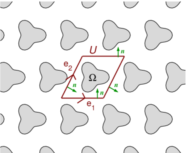
a)   b) 

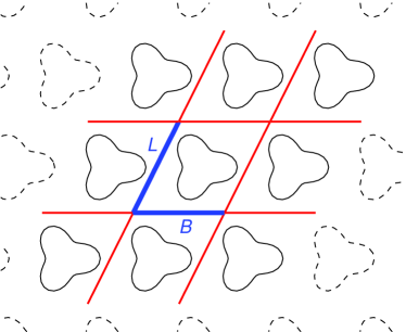
Figure 1: a) Problem geometry: an infinite dielectric crystal, in the case where the inclusion $\Omega$ lies within a parallelogram unit cell $U$. The (shaded) set of all inclusions in the lattice, denoted by $\Omega_{\Lambda}$ in the text, has refractive index $n$, while the white region has index 1. b) Sketch of our quasi-periodizing scheme: we make use of layer potentials on the left (L) and bottom (B) walls, extended to the additional segments shown, which form a skewed ‘tic-tac-toe’ board, as well as the near neighbor images of $\Omega$, outlined in solid lines.

We assume that the crystal consists of a periodic array of obstacles ($\Omega_{\Lambda}$) with refractive index $n\neq 1$, embedded in a background material with refractive index $n=1$ (denoted by $\mathbb{R}^{2}\setminus\overline{\Omega_{\Lambda}}$). We then rewrite (1) as a system of Helmholtz equations

$$(\Delta+n^{2}\omega^{2})u = 0\qquad\mbox{in }\Omega_{\Lambda}$$ (2)

$$(\Delta+\omega^{2})u = 0\qquad\mbox{in }\mathbb{R}^{2}\setminus\overline{\Omega_{\Lambda}}$$ (3)

The expression $\overline{\Omega_{\Lambda}}$, above, is used to denote the closure of the domain $\Omega_{\Lambda}$ (the union of the domain and its boundary $\partial\Omega_{\Lambda}$). In this formulation, we must also specify conditions at the material interfaces. These are derived from the required continuity of the tangential components of the electric and magnetic fields across $\partial\Omega_{\Lambda}$ [27, 28], yielding

$$u,{u_{n}}\mbox{ continuous across }\partial\Omega_{\Lambda}$$ (4)

where ${u_{n}}=\partial u/\partial n$ is the outward-pointing normal derivative.

The essential feature of doubly periodic microstructures in 2D (or triply periodic microstructures in 3D) is that, at each frequency, there may exist traveling wave solutions (Bloch waves) propagating in some direction defined by a vector ${\bf k}$.

Definition 1

Bloch waves are nontrivial solutions to (2)–(4) that are quasiperiodic, in the sense that

$$u(\textbf{x})=e^{i\textbf{k}\cdot\textbf{x}}\tilde{u}(\textbf{x})\,,$$ (5)

where $\tilde{u}$ is periodic with the lattice period and $\textbf{k}=(k_{x},k_{y})$ is real-valued. k is referred to as the Bloch wavevector.

Bloch waves characterize the bulk optical properties at frequency $\omega$; they are analogous to plane waves for free space. If such waves are absent for all directions k for a given $\omega$, then the material is said to have a band-gap [48]). The size of a band-gap is the length of the frequency interval $[\omega_{1},\omega_{2}]$ in which Bloch waves are absent. Crystal structures with a large band-gap are ‘optical insulators’ in which defects may be used as guides [28], with the potential for enabling high-speed integrated optical computing and signal processing.

Definition 2

The band-structure of a given crystal geometry is the set of parameter pairs $(\omega,\textbf{k})$ for which nontrivial Bloch waves exist.

The numerical prediction of band structure is a computationally challenging task, yet essential to the design and optimization of practical devices. It requires characterizing the nontrivial solutions to a homogeneous system of partial differential equations (2), (3) subject to homogeneous interface and periodicity conditions (4), (5) in complicated geometry. Solving this eigenvalue problem is the focus of our paper.

In the next section, we briefly review existing approaches, and in section 3, we present and test a method that relies on the quasi-periodic Green’s function. We introduce our new mathematical formulation in section 4. Numerical results are presented in section 5, and we conclude in section 6 with some remarks about the potential for wider application of this approach.

2 Existing approaches

In order to pose the band-structure problem as an eigenvalue problem on the unit cell $U$ (see Fig. 1), we will require some additional notation. The nonparallel vectors $\textbf{e}_{1},\textbf{e}_{2}\in\mathbb{R}^{2}$ define a Bravais lattice $\Lambda:=\{m\textbf{e}_{1}+n\textbf{e}_{2}:m,n\in\mathbb{Z}\}$. Given a smooth, simply connected inclusion $\Omega\subset\mathbb{R}^{2}$, we may formally define the corresponding dielectric crystal by $\Omega_{\Lambda}:=\{\Omega+\textbf{d}:\textbf{d}\in\Lambda\}$. As indicated above, we assume that $\Omega_{\Lambda}$ has refractive index $n\neq 1$, and that the background $\mathbb{R}^{2}\setminus\overline{\Omega_{\Lambda}}$ has refractive index 1. For the moment, we assume that $\overline{\Omega}\subset U$ as illustrated in Fig. 1. We will discuss the case of $\Omega$ crossing $\partial U$ in Section 5.1.

The quasi-periodicity condition (5) can be rewritten as a set of boundary conditions on the unit cell $U$, coupling the solution on the left ($L$) and right ($L+\textbf{e}_{1}$) walls, as well as on the bottom ($B$) and top ($B+\textbf{e}_{2}$) walls. More precisely, if we define

$$a:=\textbf{k}\cdot\textbf{e}_{1},\quad\alpha:=e^{ia},\qquad b:=\textbf{k}\cdot\textbf{e}_{2},\quad\beta:=e^{ib}\,,$$

then quasi-periodicity is written

$$u|_{L+\textbf{e}_{1}} = \alpha\,u|_{L}$$ (6)

$${u_{n}}|_{L+\textbf{e}_{1}} = \alpha\,{u_{n}}|_{L}$$ (7)

$$u|_{B+\textbf{e}_{2}} = \beta\,u|_{B}$$ (8)

$${u_{n}}|_{B+\textbf{e}_{2}} = \beta\,{u_{n}}|_{B}\,,$$ (9)

where the normals have the senses shown in Fig. 1.

The homogeneous equations (2)-(4), (6)-(9) define a partial differential equation (PDE) eigenvalue problem on the torus $U$. By convention, the band structure or Bloch eigenvalues are generally defined as the subset of the parameter space $\{(\omega,a,b):\omega>0,-\pi\leq a<\pi,-\pi\leq b<\pi\}$ for which nontrivial solutions $u:U\to\mathbb{C}$ exist. The earlier definition of band-structure, based on (5), allows for arbitrary values of k. It is clear, however, that one only needs to consider a single period of k’s projection onto $\textbf{e}_{1},\textbf{e}_{2}$, which we have denoted by $a,b$, to characterize the entire set $(\omega,\textbf{k})$ of nontrivial Bloch waves. This domain $\{(a,b):-\pi\leq a<\pi,-\pi\leq b<\pi\}$ is (essentially) what is referred to as the Brillouin zone.

Because the PDE is elliptic and $U$ is compact, for each k there is a discrete set of eigenvalues $\{\omega_{j}(\textbf{k})\}_{j=1}^{\infty}$, counting multiplicity, accumulating only at infinity. Each $\omega_{j}(\textbf{k})$ is continuous in k, so that the bands form sheets.

Popular numerical methods for band structure calculations are reviewed in [28]. Broadly speaking, they may be classified as either time-domain or frequency domain schemes. In the first case, an initial pulse is evolved via the full wave equation (typically using a finite-difference or finite-element approximation). If the simulation is sufficiently long, Fourier transformation in the time variable then reveals the full band structure. In the second case, the eigenvalue problem (2)-(4), (6)-(9) is discretized directly. Such frequency domain schemes can be further categorized as

1. PDE-based methods, which involve discretizing the unit cell using finite difference or finite element methods [3, 19, 20],

2. plane-wave methods which expand the function $\tilde{u}$ in (5) as a Fourier series, and apply the partial differential operator in Fourier space [28, 29],

3. semi-analytic multipole expansion methods which apply largely to cylindrical or spherical inclusions [10, 43],

4. methods which use a basis of particular solutions to the PDE at a given frequency $\omega$ and enforce both interface and boundary conditions as a linear system, such as the “multiple multipole” or “transfer-matrix” method [23, 46], and

5. boundary integral (boundary element) methods [49], which includes the method described here.

For a fixed k, methods of type (1) and (2) result in large, sparse generalized eigenvalue problems whose lowest few eigenvalues approximate the first few bands $\omega_{j}(\textbf{k})$. They have the advantage that they couple easily to existing robust linear algebraic techniques. PDE-based methods, however, require discretization of the entire cell in a manner that accurately resolves the geometry of the inclusion $\Omega$. Plane-wave methods, which perform extremely well when the index of refraction $n$ is smooth, have low order convergence when $n$ is piecewise constant, as in the present setting. Both require a large number of degrees of freedom.

Methods of type (3), (4) or (5), on the other hand, represent the solution using specialized functions (solutions of the PDE) whose dependence on $\omega$ is nonlinear. As a result, they can be much more efficient and high-order accurate, dramatically reducing the number of degrees of freedom required. Unfortunately, however, they result in a nonlinear eigenvalue problem involving all the parameters $\omega$, $a$ and $b$, and somewhat non-standard techniques are required to find values of the parameters for which the system of equations is singular [47].

We are particularly interested in using boundary integral methods (BIEs), since they easily handle jumps in the index in complicated geometry, have a well understood mathematical foundation, and can achieve rapid convergence, limited only by the order of accuracy of the quadrature rules used. High order accuracy is important, not only because of the reduction in the size of the discretized problem, but in carrying out subsequent tasks, such as sensitivity analyses [17] through the numerical approximation of derivatives, and the computation of band slopes (group velocity), and band curvatures (group dispersion).

There is surprisingly little historical literature on using BIE for band structure calculations, although the last few years have begun to see some activity in this direction (see, for example, [49]). There is, however, an extensive literature on integral equations for scattering from periodic structures, which we do not seek to review here. For some recent work and additional references, see [14, 42].

3 Integral equations based on the quasi-periodic Green’s function

An elegant approach to designing integral representations for quasiperiodic fields involves the construction of the Green’s function that imposes the desired conditions (6)-(9) exactly. We first need some definitions [16, 41]. At wavenumber $\omega>0$, the free space Green’s function for the Helmholtz equation, $G$ is defined by $-(\Delta+\omega^{2})G=\delta_{{\bm{0}}}$ where $\delta_{\bm{0}}$ is the Dirac delta function centered at the origin. In 2D, this yields

$$G(\textbf{x})=G^{(\omega)}(\textbf{x})=\frac{i}{4}H_{0}^{(1)}(\omega|\textbf{x}|),\qquad\textbf{x}\in\mathbb{R}^{2}\setminus\{{\bm{0}}\},$$ (10)

where $H_{0}^{(1)}$ is the outgoing Hankel function of order zero. By formally summing over images of the Green’s function placed on the lattice $\Lambda$, with correctly assigned phases, we get an explicit expression for the quasi-periodic Greens function

$$G_{{\mbox{\tiny\rm QP}}}(\textbf{x})=\sum_{\textbf{d}\in\Lambda}e^{i\textbf{k}\cdot\textbf{d}}G(\textbf{x}-\textbf{d})=\sum_{m,n\in\mathbb{Z}}\alpha^{m}\beta^{n}G(\textbf{x}-m\textbf{e}_{1}-n\textbf{e}_{2})\,.$$ (11)

We leave it to the reader to verify that $G_{{\mbox{\tiny\rm QP}}}$ does, indeed, satisfy (6)-(9). One small caveat: the series in (11) is conditionally convergent for real $\omega$. The physically meaningful limit is taken by assuming some dissipation $\omega=\omega+i\varepsilon$ in the limit $\varepsilon\rightarrow 0^{+}$ (see [18] for a more detailed discussion). It will be useful to distinguish between the copy of the Green’s function sitting in the unit cell $U$ and the set of all other images. For this, we define the “regular” part of the quasi-periodic Green’s function by

$$G_{{\mbox{\tiny\rm QP}}}^{r}(\textbf{x})=\sum_{\begin{subarray}{c}m,n\in\mathbb{Z}\\ (m,n)\neq(0,0)\end{subarray}}\alpha^{m}\beta^{n}G(\textbf{x}-m\textbf{e}_{1}-n\textbf{e}_{2})\,.$$ (12)

This function is a smooth solution to the Helmholtz equation within $U$ and clearly satisfies

$$G_{{\mbox{\tiny\rm QP}}}(\textbf{x})=G(\textbf{x})+G_{{\mbox{\tiny\rm QP}}}^{r}(\textbf{x})~{}.$$ (13)

A spectral representation also exists [9, 18], built from the plane-wave eigenfunctions of the quasi-periodic torus $U$:

$$G_{{\mbox{\tiny\rm QP}}}(\textbf{x})=\frac{1}{\mbox{Vol}(U)}\sum_{\textbf{q}\in\Lambda^{*}}\frac{e^{i(\textbf{k}+\textbf{q})\cdot\textbf{x}}}{|\textbf{k}+\textbf{q}|^{2}-\omega^{2}}\,.$$ (14)

Here, $\Lambda^{\ast}:=\{m\textbf{r}_{1}+n\textbf{r}_{2}:m,n\in\mathbb{Z}\}$ is the reciprocal lattice with vectors $\textbf{r}_{j}$ defined by ${\textbf{e}}_{i}\cdot\textbf{r}_{j}=2\pi\delta_{ij}$ for $i,j=1,2$. From the denominators in (14) it is clear that $G_{{\mbox{\tiny\rm QP}}}$ may blow up for specific combinations of $\omega$ and k. The quasiperiodic Green’s function is, in fact, well-defined if and only if those parameters satisfy the following non-resonance condition.

Definition 3 (empty resonance)

A parameter set $(\omega,\textbf{k})$, equivalently $(\omega,a,b)$, is empty resonant if $\omega=|\textbf{k}+\textbf{q}|$ for some $\textbf{q}\in\Lambda^{\ast}$, otherwise it is empty non-resonant.

Our terminology comes from the fact that the blow-up in $G_{{\mbox{\tiny\rm QP}}}$ is physically the resonance of the ‘empty’ unit cell $U$, with refractive index 1 everywhere and quasi-periodic boundary conditions. That is, $G_{{\mbox{\tiny\rm QP}}}$ is undefined if and only if $(\omega,a,b)$ lies on the band structure of the empty unit cell. The blow-up of the Green’s function is less apparent from (11), but is manifested in the divergence of the series, even in the limit $\omega=\omega+i\varepsilon$ with $\varepsilon\rightarrow 0^{+}$.

It will be convenient sometimes to refer to a Green’s function as a function of two variables, with $G(\textbf{x},\textbf{y}):=G(\textbf{x}-\textbf{y})$, and $G_{{\mbox{\tiny\rm QP}}}(\textbf{x},\textbf{y}):=G_{{\mbox{\tiny\rm QP}}}(\textbf{x}-\textbf{y})$. Then, for each $\textbf{y}\in\mathbb{R}^{2}$, the function $G_{{\mbox{\tiny\rm QP}}}(\cdot,\textbf{y})$ is quasi-periodic.

We now represent solutions to the PDE eigenvalue problem (2)-(4), (6)-(9) by the layer potentials,

$$u\;=\;\left\{\begin{array}[]{ll}{\cal S}^{(n\omega)}\sigma+{\cal D}^{(n\omega)}\tau&\mbox{in }\Omega\\ {\cal S}^{(\omega)}_{\mbox{\tiny QP}}\sigma+{\cal D}^{(\omega)}_{\mbox{\tiny QP}}\tau&\mbox{in }U\setminus\overline{\Omega}\end{array}\right.$$ (15)

where the usual single and double layer densities [16] at any wavenumber $\omega>0$ are defined by

$$({\cal S}^{(\omega)}\sigma)(\textbf{x}) = \int_{\partial\Omega}G^{(\omega)}(\textbf{x},\textbf{y})\sigma(\textbf{y})ds_{\textbf{y}}$$ (16)

$$({\cal D}^{(\omega)}\tau)(\textbf{x}) = \int_{\partial\Omega}\frac{\partial G^{(\omega)}}{\partial n_{\textbf{y}}}(\textbf{x},\textbf{y})\tau(\textbf{y})ds_{\textbf{y}}$$ (17)

and their quasi-periodized versions are likewise

$$({\cal S}^{(\omega)}_{\mbox{\tiny QP}}\sigma)(\textbf{x}) = \int_{\partial\Omega}G_{{\mbox{\tiny\rm QP}}}^{(\omega)}(\textbf{x},\textbf{y})\sigma(\textbf{y})ds_{\textbf{y}}$$ (18)

$$({\cal D}^{(\omega)}_{\mbox{\tiny QP}}\tau)(\textbf{x}) = \int_{\partial\Omega}\frac{\partial G_{{\mbox{\tiny\rm QP}}}^{(\omega)}}{\partial n_{\textbf{y}}}(\textbf{x},\textbf{y})\tau(\textbf{y})ds_{\textbf{y}}~{}.$$ (19)

Here $ds$ is the usual arc length measure on ${\partial\Omega}$, and the derivatives are with respect to the second variable in the outward surface normal direction at y. It is clear [16] that the above four fields satisfy the Helmholtz equation at wavenumber $\omega$ in both $\Omega$ and $U\setminus\overline{\Omega}$. Note that we have chosen a non-periodized representation within the inclusion $\Omega$ in (15), which has some analytic advantages (see Theorem 4 and the last paragraph in the Appendix).

Since $u$ in (15) satisfies (2), (3), and (6)-(9), all that remains is to solve for densities $\sigma$, $\tau$ such that the matching conditions (4) are satisfied, which we now address.

Using superscripts $+$ and $-$ to denote limiting values on ${\partial\Omega}$, approaching from the positive and negative normal side respectively, we use the field (15) and the standard jump relations for single and double layer potentials [16, 22] to write

$$\left[\begin{matrix}u^{+}-u^{-}\\ {u_{n}}^{+}-{u_{n}}^{-}\end{matrix}\right]\;=\;\left(\,\left[\begin{matrix}I&0\\ 0&I\end{matrix}\right]+\left[\begin{matrix}D^{(\omega)}_{\mbox{\tiny QP}}-D^{(n\omega)}&S^{(n\omega)}-S_{\mbox{\tiny QP}}^{(\omega)}\\ T_{\mbox{\tiny QP}}^{(\omega)}-T^{(n\omega)}&D^{(n\omega)\,\ast}-D^{(\omega)\,\ast}_{\mbox{\tiny QP}}\end{matrix}\right]\,\right)\left[\begin{matrix}\tau\\ -\sigma\end{matrix}\right]\;=:\;A_{{\mbox{\tiny\rm QP}}}\eta$$ (20)

Here $I$ is the identity operator, while $S$ and $D$ are defined to be the limiting boundary integral operators (maps from $C({\partial\Omega})\to C({\partial\Omega})$) with the kernels ${\cal S}$ and ${\cal D}$ interpreted in the principal value sense. ($S$ is actually weakly singular so the limit is already well defined. A standard calculation [16, 22] shows that $D$ is weakly singular as well). The hypersingular operator $T$ has the kernel $\frac{\partial^{2}G(\textbf{x},\textbf{y})}{\partial n_{\textbf{x}}\partial n_{\textbf{y}}}$ and is unbounded as a map from $C({\partial\Omega})\to C({\partial\Omega})$. In these definitions, as in (16)-(19), it is implied that $G$ inherits the appropriate superscripts and subscripts from $S$, $D$ and $T$. Finally, $\ast$ indicates the adjoint. The amounts by which the material matching conditions fail to be satisfied,

$$m\;:=\;\left[\begin{matrix}u^{+}-u^{-}\\ {u_{n}}^{+}-{u_{n}}^{-}\end{matrix}\right]~{},$$ (21)

is a column vector of functions which we call the mismatch. We summarize the linear system (20) by $m=A_{{\mbox{\tiny\rm QP}}}\eta$ where $\eta:=[\tau;-\sigma]$. It is important to note that the difference of hypersingular kernels, ${T_{\mbox{\tiny QP}}^{(\omega)}-T^{(n\omega)}}$, in (20) is only weakly singular [16, Sec. 3.8]. This cancellation, achieved here by using the same pair of densities inside as outside the inclusion, is well known [44]. The result is that $A_{{\mbox{\tiny\rm QP}}}$ is a compact perturbation of the identity and (20) is a Fredholm system of integral equations of the second kind.

In the above scheme, we might hope that if it is possible to find nontrivial densities $\eta$ whose field $u$ gives zero mismatch $m$ for a set of parameters $(\omega,a,b)$, then that set is a Bloch eigenvalue. Indeed (as with the case of simpler domain eigenvalue problems [39, Sec. 8]) we have a stronger result.

Theorem 4

Let $(\omega,a,b)$ be empty non-resonant. Then $(\omega,a,b)$ is a Bloch eigenvalue if and only if $\operatorname{Null}A_{{\mbox{\tiny\rm QP}}}\neq\{0\}$ .

The proof occupies Appendix A. This suggests the core of a numerical scheme: at each of a sampling (e.g. a grid) of parameters $(\omega,a,b)$, find the lowest singular value $\sigma_{\mbox{\tiny min}}(\tilde{A}_{{\mbox{\tiny\rm QP}}})$ of a matrix discretization $\tilde{A}_{{\mbox{\tiny\rm QP}}}$ of $A_{{\mbox{\tiny\rm QP}}}$. The band structure will then be found where $\sigma_{\mbox{\tiny min}}(\tilde{A}_{{\mbox{\tiny\rm QP}}})$ is close to zero.

3.1 Discretization of the integral operators

Since the goal of this work is to explore periodization, we limit ourselves to the simplest case of ${\partial\Omega}$ being smooth. The methods of this paper extend without much effort to other shapes, but the quadrature issues become more involved. Recalling (13), note that the kernels in (20) are the sum of a component due to $G$ which is weakly singular, plus the remainder due to $G_{{\mbox{\tiny\rm QP}}}^{r}$ which is smooth (analytic). We will make use of a Nyström discretization using the spectral quadrature scheme of Kress [31] for $G$ and the trapezoidal rule for $G_{{\mbox{\tiny\rm QP}}}^{r}$.

We first remind the reader of the periodic trapezoidal Nyström scheme [33], in the context of a general second kind boundary integral equation

$$\mu(\textbf{x})+\int_{\partial\Omega}k(\textbf{x},\textbf{y})\mu(\textbf{y})ds_{\textbf{y}}=f(\textbf{x}),\qquad\textbf{x}\in{\partial\Omega},$$

where ${\partial\Omega}$ is parametrized by the $2\pi$-periodic analytic function $\textbf{z}:[0,2\pi)\to\mathbb{R}^{2}$. Changing variable gives

$$\mu(s)+\int_{0}^{2\pi}K(s,t)\mu(t)dt=f(s),\qquad s\in[0,2\pi),$$

where $K(s,t):=k(\textbf{z}(s),\textbf{z}(t))\,|\textbf{z}^{\prime}(t)|$ and $\textbf{z}^{\prime}=d\textbf{z}/dt$. Choosing $N$ quadrature points $t_{j}=2\pi j/N$ with equal weights $2\pi/N$ gives the $N$-by-$N$ linear system for the unknowns $\mu^{(N)}_{j}$, which approximate the exact values $\mu(t_{j})$, as

$$\mu^{(N)}_{k}+\frac{2\pi}{N}\sum_{j=1}^{N}K(t_{k},t_{j})\mu^{(N)}_{j}\;=\;f(t_{k}),\qquad k=1,\dots,N~{}.$$ (22)

By Anselone’s theory of collectively compact operators [33], the convergence of errors $\bigl{|}\mu^{(N)}_{j}-\mu(t_{j})\bigr{|}$ inherits the order of the quadrature scheme applied to the exact integrand $K(s,\cdot)\mu$, which is analytic when $k$ and $f$ are.

Remark 5

For analytic integrands, the periodic trapezoidal rule has exponential convergence with error $O(e^{-2\gamma N})$ where $\gamma$ is the smallest distance from the real axis of any singularity in the analytic continuation of the integrand. [33, Thm. 12.6].

The above discretization is used to populate the matrix entries in (20) that are due to the smooth compoment $G_{{\mbox{\tiny\rm QP}}}^{r}$. (We explain how to compute this kernel itself in Section 3.2.)

For non-smooth kernels, such as $G$, the rule (22) must be replaced by a quadrature that correctly accounts for the singularity in order to retain high order accuracy. There are a variety of such schemes, such as those of [2, 24, 30]. By fixing the order of accuracy, they allow for straightforward coupling to fast multipole acceleration [12, 13, 14, 42] by making local modifications of a simple underlying quadrature rule (such as the trapezoidal rule or a composite Gaussian rule). In the present context, we ignore such considerations and use a global rule due to Kress [31] that achieves spectral accuracy in the logarithmically singular case.

The essential idea of Kress’ scheme (after transformation of variables to the interval $[0,2\pi]$) is to split a logarithmically singular kernel $K(s,t)$ in the form

$$K(s,t)=\log\left(4\sin^{2}\frac{s-t}{2}\right)K_{1}(s,t)+K_{2}(s,t)$$ (23)

with $K_{1}$ and $K_{2}$ periodic and analytic. $K_{2}$ is (again) handled with the trapezoidal rule. For $K_{1}$, the Kussmaul-Martensen quadrature rule is spectrally accurate:

$$\int_{0}^{2\pi}\log\left(4\sin^{2}\frac{s-t}{2}\right)g(t)dt\approx\sum_{j=1}^{N}R^{(N)}_{j}(s)g(t_{j})$$ (24)

with quadrature weights (deriving from the Fourier series of the log factor) given by

$$R^{(N)}_{j}(s)\;=\;-\sum_{m=1}^{N/2-1}\frac{2}{m}\cos m(s-t_{j})\;-\;\frac{2}{N}\cos\frac{N}{2}(s-t_{j})~{}.$$ (25)

Thus, the matrix elements in discretizing (23) are $K(t_{k},t_{j})=R^{(N)}_{|j-k|}(0)K_{1}(t_{k},t_{j})+K_{2}(t_{k},t_{j})$. Finally, it is always the difference of two hypersingular operators $T$ that appears in the integral equation (20). This difference is only logarithmically singular, so that Kress’ rule can be used for every block of (20). We refer the reader to [31] for further details.

In summary, a matrix discretization $\hat{A}_{\mbox{\tiny QP}}$ of $A_{{\mbox{\tiny\rm QP}}}$ is formed by using the above quadrature rules for each of the 2-by-2 integral operator blocks in (20). This matrix maps density values to field values. However, in order to create a matrix whose singular values approximate those of $A_{{\mbox{\tiny\rm QP}}}$ we must instead normalize such that $2N$-dimensional Euclidean 2-norms correctly approximate $L^{2}({\partial\Omega})$-norms. This is done by symmetrizing using quadrature weights to give our final matrix

$$\tilde{A}_{\mbox{\tiny QP}}=W^{1/2}\hat{A}_{\mbox{\tiny QP}}W^{-1/2}$$ (26)

where $W$ is diagonal with diagonal elements $w_{j}=w_{j+N}=(2\pi/N)|\textbf{z}^{\prime}(t_{j})|$, for $j=1,\ldots,N$.

The net result of the preceding discussion is that with the use of specialized quadratures on smooth boundaries, the singular values of $\tilde{A}_{\mbox{\tiny QP}}$ are spectrally accurate approximations to those of $A_{{\mbox{\tiny\rm QP}}}$. We demonstrate this convergence for a small trefoil-shaped inclusion in Fig. 2a; the convergence is spectral, until the error is approximately machine precision times the matrix 2-norm. The rate appears to be faster at a Bloch eigenvalue (in this case on the fourth band) than far from one. Fig. 2b shows that the minimum locates the parameter $b$ to 14 digit accuracy for $N\geq 70$.

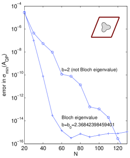
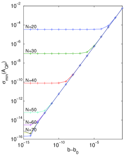
a)   b)   c)

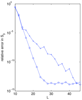
Figure 2: Convergence for quasi-periodic Greens function scheme of Sec. 3. a) Absolute error in $\sigma_{\mbox{\tiny min}}(\tilde{A}_{\mbox{\tiny QP}})$ vs $N$ the number of quadrature nodes on ${\partial\Omega}$, for Bloch parameters $a=\pi/2$ and the two different $b$ values labeled. The unit cell with $\textbf{e}_{1}=(1,0)$, $\textbf{e}_{2}=(0.4,1)$, and inclusion, described by the radial function $r(\theta)=0.2(1+0.3\cos 3\theta)$, are shown in the inset. Index is $n=3$ and frequency $\omega=4.5$. For $b=2$, error is taken relative to the converged value $0.01879908530381247$; for $b=b_{0}$, relative to 0. The matrix $\tilde{A}_{\mbox{\tiny QP}}$ has 2-norm of about 25. b) $\sigma_{\mbox{\tiny min}}(\tilde{A}_{\mbox{\tiny QP}})$ vs difference in parameter $b$ from the Bloch eigenvalue $b_{0}$, for several different numbers of quadrature points $N$. Note the horizontal log scale. This shows that it is the convergence rate at the Bloch eigenvalue that controls the accuracy with which the minimum can be found. c) Relative error ($+$ symbols) in evaluation of lattice sum $S_{3}$ by the method of Sec. 3.2 vs the maximum order $L$ in (27). Parameters are as in Table II of [38], whose claim $S_{3}=2.13097899279352+5.66537068305984i$ is taken as the true value. Also, relative error ($\circ$ symbols) for $\tilde{S}_{3}$ which excludes the $3\times 3$ block of neighbors (parameters are the same; true value is taken as the converged value at $L=50$).

3.2 New method for evaluation of the quasi-periodic Greens function

In order to compute the elements of $\tilde{A}_{\mbox{\tiny QP}}$, one must evaluate $G_{{\mbox{\tiny\rm QP}}}^{r}$ defined by (12); in this section, we present a surprisingly simple (and apparently new) method for this. Since the sums (11) and (14) converge too slowly to be numerically useful, many sophisticated schemes have been devised. Some of these are based on the Fourier representation (such as [9]), but most are based on the observation that

$$G_{{\mbox{\tiny\rm QP}}}^{r}(r,\theta)=\sum_{l=-L}^{L}S_{l}J_{l}(\omega r)e^{il\theta}~{},$$ (27)

where $(r,\theta)$ are the usual polar coordinates, and $J_{l}$ the regular Bessel function of order $l$. As $L\to\infty$, this expression is uniformly convergent in the unit cell $U$, as long as there exists a circle about the origin which contains $\overline{U}$ but encloses no points in $\Lambda\setminus\{{\bm{0}}\}$. The coefficients $S_{l}$ in this expansion are know as lattice sums, given by

$$S_{l}=\sum_{\begin{subarray}{c}m,n\in\mathbb{Z}\\ (m,n)\neq(0,0)\end{subarray}}\alpha^{m}\beta^{n}\,H_{l}^{(1)}(\omega r_{mn})e^{-il\theta_{mn}},$$

where $(r_{mn},\theta_{mn})$ are the polar coordinates of $m\textbf{e}_{1}+n\textbf{e}_{2}$, and $H_{l}^{(1)}$ is the outgoing Hankel function of order $l$. Thus, the issue of evaluating $G_{{\mbox{\tiny\rm QP}}}^{r}$ has been reduced to that of tabulating the lattice sums. This problem itself has a substantial literature (see, for example, [15, 18, 34, 38, 40]). Nevertheless, very few papers discuss the problem of empty resonances, at which point the lattice sums $S_{l}$ blow up. One notable exception is the work of Linton and Thompson [35], who analyze this blowup for periodic one-dimensional arrays in two dimensional scattering. They also propose a regularization method to overcome it.

We present here the construction of a small linear system whose solution yields the lattice sums rather easily (away from empty resonances). In physical terms, we compute the field induced by the free-space Green’s function $G$, determine how it fails to satisfy quasi-periodicity, and use the representation (27) to enforce quasi-periodicity numerically. More precisely, given a field $u$, we define the discrepancy by

$$d\;=\;\left[\begin{matrix}f\\ f^{\prime}\\ g\\ g^{\prime}\end{matrix}\right]\;:=\;\left[\begin{array}[]{l}u|_{L}-\alpha^{-1}u|_{L+\textbf{e}_{1}}\\ {u_{n}}|_{L}-\alpha^{-1}{u_{n}}|_{L+\textbf{e}_{1}}\\ u|_{B}-\beta^{-1}u|_{B+\textbf{e}_{2}}\\ {u_{n}}|_{B}-\beta^{-1}{u_{n}}|_{B+\textbf{e}_{2}}\end{array}\right]~{}.$$ (28)

We can interpret $f$, $f^{\prime}$ as functions on wall $L$ and $g$, $g^{\prime}$ as functions on wall $B$. We construct a $4M$-component column vector ${\bm{d}}$ by sampling these four functions at Gaussian quadrature points $\{\textbf{y}^{(L)}_{m}\}_{m=1}^{M}$ on $L$, and $\{\textbf{y}^{(B)}_{m}\}_{m=1}^{M}$ on $B$. If we let the field $u(\textbf{x})=G(\textbf{x})$, then for $m=1,\ldots,M$, the $m$th element of ${\bm{d}}$ is $G(\textbf{y}^{(L)}_{m})-\alpha^{-1}G(\textbf{y}^{(L)}_{m}+\textbf{e}_{1})$. The remaining $3M$ entries in ${\bm{d}}$ are computed in the analogous fashion.

Now let $H$ be a (complex) matrix of size $4M\times(2L+1)$, defined as follows. For $l=-L,\ldots,L$, fill the $(l+L+1)$th column in the same manner as ${\bm{d}}$, but using the field $u(\textbf{x})=J_{l}(\omega r)e^{il\theta}$. Letting ${\bm{s}}:=\{S_{l}\}_{l=-L}^{L}$, it is straightforward to verify that the linear system

$$H{\bm{s}}=-{\bm{d}}$$ (29)

yields values for the lattice sums that annihilate the discrepancy induced by the source $G$. We solve the linear system in the least squares sense. This has to be done with some care, since the Bessel functions $J_{l}$ become exponentially small for large $l$. A simple fix is to right-precondition the system by scaling the $(l+L+1)$th column of $H$ by the factor $\rho_{l}:=1/J_{l}(\min[\omega R,l])$, where $R:=\max_{\textbf{x}\in U}|\textbf{x}|$ is the unit cell radius. The entire procedure may be interpreted as finding the representation (27) which minimizes the $L^{2}$-norm of the discrepancy of the resulting $G_{{\mbox{\tiny\rm QP}}}$.

Fig. 2b shows that the error in evaluating $S_{l}$, for $l=3$, has exponential convergence in $L$. We fixed $M=24$ (large enough that further increase had no effect). 14 digits of relative accuracy are achieved for $L\geq 46$, comparable in accuracy to [38]. Although the maximum achievable accuracy for $S_{l}$ deteriorates exponentially as $|l|$ increases, the resulting accuracy of $G_{{\mbox{\tiny\rm QP}}}^{r}$ computed via (27) is close to 14 digits everywhere in $U$. We do not claim that our method is optimal in terms of speed (although at 0.05 sec to solve for all $S_{l}$ values, it is adequate), merely that it is accurate, convenient and robust. To our knowledge it has not been proposed in the literature.

The convergence rate in the boundary $L^{2}$-norm of expansions such as (27) depends on the (conformal) distance from the domain to the nearest field singularity (a result of Vekua’s theory and approximation in the complex plane [8, Ch. 6]). Thus, the rate may be improved by increasing this distance by removing the rest of the $3\times 3$ block of nearest neighbors from the lattice sum, and representing

$$\tilde{G}_{{\mbox{\tiny\rm QP}}}^{r}(\textbf{x})\;:=\!\!\sum_{(j,k)\;\in\;\mathbb{Z}^{2}\setminus\{-1,0,1\}^{2}}\!\!\!\!\alpha^{j}\beta^{k}G(\textbf{x}-j\textbf{e}_{1}-k\textbf{e}_{2})=\sum_{l=-L}^{L}\tilde{S}_{l}J_{l}(\omega r)e^{il\theta}~{}.$$ (30)

To solve for $\{\tilde{S}_{l}\}$, the right-hand side of the linear system is now chosen to be the direct summation of these neighbors, $u(\textbf{x})=\tilde{G}(\textbf{x}):=\sum_{j,k\in\{-1,0,1\}}\alpha^{j}\beta^{k}G(\textbf{x}-j\textbf{e}_{1}-k\textbf{e}_{2})$. We may then evaluate $G_{{\mbox{\tiny\rm QP}}}=\tilde{G}+\tilde{G}_{{\mbox{\tiny\rm QP}}}^{r}$. As Fig. 2c shows, the convergence rate for $\tilde{S}_{l}$, and hence for $G_{{\mbox{\tiny\rm QP}}}$, is now a factor 2–3 better. Hence we use this method below, fixing $L=30$.

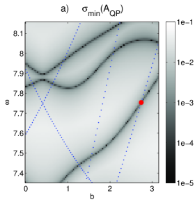
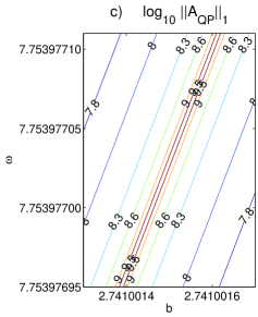
Figure 3: Breakdown of quasi-periodic Greens function scheme, for the system of Fig. 2a except with $\textbf{e}_{2}=(0.5,1)$. a) Minimum singular value of $\tilde{A}_{{\mbox{\tiny\rm QP}}}$ vs $b=\textbf{k}\cdot\textbf{e}_{2}$ and $\omega$, as a log density plot over a slice with fixed $a=0.8$. Dark curves indicate the band structure, and superimposed dotted lines the ‘empty’ band structure where $G_{{\mbox{\tiny\rm QP}}}$ blows up. b) Zooming in by a factor of $10^{7}$ to the region shown by the dot in a), showing failure to resolve band structure at the intersection. c) log 1-norm of the matrix $\tilde{A}_{\mbox{\tiny QP}}$ plotted over the same region as b); it is of order the inverse of the distance to the empty band structure.

3.3 The empty resonance problem

Given a photonic crystal (inclusion $\Omega$ with index $n$), using the methods of Sections 3.1 and 3.2 we are able to construct the matrix $\tilde{A}_{{\mbox{\tiny\rm QP}}}$ for any given frequency and Bloch parameters $(\omega,a,b)$. Fig. 3a shows the minumum singular value of this matrix as a function over the $(b,\omega)$ plane, for constant $a$: the band structure is visible as the zeros of this function. We have also superimposed the band structure of the empty unit cell (dotted lines). Theorem 4 guarantees that, away from the empty unit cell band structure, no spurious modes will be found, and that no modes are missed.

However, zooming in to one of the many intersections of the two sets of curves (Fig. 3b), we see that in the neighborhood of the empty band structure, the desired singular values take on arbitrary fluctuating values that obscure the theoretical behavior near their intersection. This prevents any attempt to locate the desired zero set to an accuracy better than $O(\sqrt{\varepsilon_{\mbox{\tiny mach}}})$, where $\varepsilon_{\mbox{\tiny mach}}$ is the machine precision. As Fig. 3c shows, this is explained by the blowup of the entries of the matrix $\tilde{A}_{{\mbox{\tiny\rm QP}}}$ as one approaches the empty band structure. This, in turn, causes unbounded roundoff error when computing small singular values in finite-precision arithmetic.

Remark 6

The above demonstrates a fundamental flaw inherent in the use of the quasi-periodic Greens function in band structure problems; there are empty-resonant parameter sets (sheets in the space $(\omega,a,b)$) where the desired band structure cannot be computed. Furthermore, loss of accuracy is inevitable near these parameter sets.

This motivates the development of a more robust scheme.

4 Periodizing using auxiliary densities on the unit cell walls

4.1 Inclusion images and a new linear system

Section 3.2 illustrated the fact, well known in the fast multipole literature [6, 14, 12, 13, 18], that summing the nearest neighbors directly (i.e. excluding them from the quasi-periodic field representation) results in much improved convergence rates. This motivates defining generalizations of (16) and (17) that include summation over the appropriately phased $3\times 3$ nearest neighbor images, as shown in Fig. 1b,

$$(\tilde{\cal S}^{(\omega)}\sigma)(\textbf{x}) = \int_{{\partial\Omega}}\sum_{j,k\in\{-1,0,1\}}\!\!\alpha^{j}\beta^{k}G^{(\omega)}(\textbf{x},\textbf{y}+j\textbf{e}_{1}+k\textbf{e}_{2})\,\sigma(\textbf{y})ds_{\textbf{y}}$$ (31)

$$(\tilde{\cal D}^{(\omega)}\tau)(\textbf{x}) = \int_{{\partial\Omega}}\sum_{j,k\in\{-1,0,1\}}\!\!\alpha^{j}\beta^{k}\frac{\partial G^{(\omega)}}{\partial n_{\textbf{y}}}(\textbf{x},\textbf{y}+j\textbf{e}_{1}+k\textbf{e}_{2})\,\tau(\textbf{y})ds_{\textbf{y}}$$ (32)

We now choose a layer potential representation for $u$ that involves only free space kernels:

$$u\;=\;\left\{\begin{array}[]{ll}{\cal S}^{(n\omega)}\sigma+{\cal D}^{(n\omega)}\tau&\mbox{in }\Omega\\ \tilde{\cal S}^{(\omega)}\sigma+\tilde{\cal D}^{(\omega)}\tau+u_{\mbox{\tiny QP}}[\xi]&\mbox{in }U\setminus\overline{\Omega}\end{array}\right.$$ (33)

The auxiliary field $u_{\mbox{\tiny QP}}$ will be represented by a new set of layer potentials that lie on the “tic-tac-toe” stencil of Fig. 1b, consisting of the boundary of $U$ and its closest extensions, none lying in the interior of $U$. We will return to this in section 4.2. For the moment, let us denote the unknown densities that determine $u_{\mbox{\tiny QP}}$ by $\xi$. By construction, the representation (33) satisfies (2) and (3) in $U$, so that it remains only to impose both the matching/continuity conditions (4) and quasi-periodicity (6)-(9). Imposing the mismatch $m$ defined by (21) and the discrepancy $d$ defined by (28) on $u$, the unknowns in (33) must satisfy a linear system of the form:

$$E\left[\begin{matrix}\eta\\ \xi\end{matrix}\right]:=\left[\begin{matrix}A&B\\ C&Q\end{matrix}\right]\left[\begin{matrix}\eta\\ \xi\end{matrix}\right]=\left[\begin{matrix}m\\ d\end{matrix}\right]~{},$$ (34)

where, as before, $\eta:=[\tau;-\sigma]$, We will describe the operators $A$, $B$, $C$, and $Q$ in more detail shortly. For the moment, note that if there exists a density $[\eta;\xi]$ which generates a nontrivial field with vanishing mismatch and discrepancy, then it is a solution to (2)-(4) and (6)-(9) and the corresponding parameters $(\omega,a,b)$ must be a Bloch eigenvalue. Numerical evidence supports the following stronger claim, the analog of Theorem 4.

Conjecture 7

$(\omega,a,b)$ is a Bloch eigenvalue if and only if $\operatorname{Null}E\neq\{0\}$.

This suggests, as in Section 3, computing the band structure by locating the parameter families where (a discretization of) $E$ is singular. The point of the new scheme is that it should be robust; if the conjecture holds, then (in contrast to the quasiperiodic Green’s function approach), there will be no spurious parameter values where the method breaks down.

To discuss the operators in $E$, we need some additional notation. We assume that the wavenumber $\omega$ and quasiperiodicity parameters $(a,b)$ are given. Let $W$ be a curve in $\mathbb{R}^{2}$ on which single and double layer densities are defined, with the corresponding potentials written as

$$({\cal S}_{W}\sigma)(\textbf{x}) = \int_{W}G(\textbf{x},\textbf{y})\sigma(\textbf{y})ds_{\textbf{y}}$$ (35)

$$({\cal D}_{W}\tau)(\textbf{x}) = \int_{W}\frac{\partial G}{\partial n_{\textbf{y}}}(\textbf{x},\textbf{y})\tau(\textbf{y})ds_{\textbf{y}}\,.$$ (36)

Letting $V$ be a (possibly distinct) target curve in $\mathbb{R}^{2}$, we define the operators

$$({S}_{V,W}\sigma)(\textbf{x}) = \int_{W}G(\textbf{x},\textbf{y})\sigma(\textbf{y})ds_{\textbf{y}}\qquad\textbf{x}\in V$$ (37)

$$({D}_{V,W}\tau)(\textbf{x}) = \int_{W}\frac{\partial G}{\partial n_{\textbf{y}}}(\textbf{x},\textbf{y})\tau(\textbf{y})ds_{\textbf{y}}\qquad\textbf{x}\in V$$ (38)

$$({D}^{\ast}_{V,W}\sigma)(\textbf{x}) = \int_{W}\frac{\partial G}{\partial n_{\textbf{x}}}(\textbf{x},\textbf{y})\sigma(\textbf{y})ds_{\textbf{y}}\qquad\textbf{x}\in V$$ (39)

$$({T}_{V,W}\tau)(\textbf{x}) = \int_{W}\frac{\partial^{2}G}{\partial n_{\textbf{x}}\partial n_{\textbf{y}}}(\textbf{x},\textbf{y})\tau(\textbf{y})ds_{\textbf{y}}\qquad\textbf{x}\in V~{}.$$ (40)

When $V=W$, these operators are to be understood in the principal value sense. By analogy with (31), (32), versions of these operators whose kernels include the phased sum over $3\times 3$ images of the source are indicated with a tilde ($\sim$): that is, $\tilde{S}_{V,W},\tilde{D}_{V,W},\tilde{D}^{\ast}_{V,W}$, and $\tilde{T}_{V,W}$.

We are now in a position to provide explicit expressions for the operators $A,B,C,Q$ in (34). Comparing (33) to (15), it is clear that the operator $A$ is the same as $A_{{\mbox{\tiny\rm QP}}}$ in (20) but with the replacement of $S_{\mbox{\tiny QP}}^{(\omega)}$, $D_{\mbox{\tiny QP}}^{(\omega)}$ and $T_{\mbox{\tiny QP}}^{(\omega)}$, by $\tilde{S}_{{\partial\Omega},{\partial\Omega}}$, $\tilde{D}_{{\partial\Omega},{\partial\Omega}}$ and $\tilde{T}_{{\partial\Omega},{\partial\Omega}}$, respectively. It is straightforward to verify that $A$ is a compact perturbation of the identity.

The operator $C$ describes the effect of the inclusion densities on the discrepancy $d$. Its eight sub-blocks are found by inserting (31) and (32) into (33) then evaluating (28), giving

$$C\;=\;\begin{bmatrix}\tilde{D}_{L,{\partial\Omega}}\!-\alpha^{-1}\tilde{D}_{L+\textbf{e}_{1},{\partial\Omega}}&-\tilde{S}_{L,{\partial\Omega}}\!+\alpha^{-1}\tilde{S}_{L+\textbf{e}_{1},{\partial\Omega}}\\ \tilde{T}_{L,{\partial\Omega}}\!-\alpha^{-1}\tilde{T}_{L+\textbf{e}_{1},{\partial\Omega}}&-\tilde{D}^{\ast}_{L,{\partial\Omega}}\!+\alpha^{-1}\tilde{D}^{\ast}_{L+\textbf{e}_{1},{\partial\Omega}}\\ \tilde{D}_{B,{\partial\Omega}}\!-\beta^{-1}\tilde{D}_{B+\textbf{e}_{2},{\partial\Omega}}&-\tilde{S}_{B,{\partial\Omega}}\!+\beta^{-1}\tilde{S}_{B+\textbf{e}_{2},{\partial\Omega}}\\ \tilde{T}_{B,{\partial\Omega}}\!-\beta^{-1}\tilde{T}_{B+\textbf{e}_{2},{\partial\Omega}}&-\tilde{D}^{\ast}_{B,{\partial\Omega}}\!+\beta^{-1}\tilde{D}^{\ast}_{B+\textbf{e}_{2},{\partial\Omega}}\end{bmatrix}$$

Consider now the any of the four upper sub-blocks of $C$. There are nine phased copies of ${\partial\Omega}$ which contribute to the field on the left ($L$) and right ($L+\textbf{e}_{1}$) wall. From symmetry and translation invariance considerations, however, it is easy to check that the contributions from the six left-most images on $L$ (dotted curves in Fig. 4a) are equal to the contributions of the six right-most images on $L+\textbf{e}_{1}$ (dotted curves in Fig. 4b). In the $(1,1)$ sub-block, for example, we have:

$$\tilde{D}_{L,{\partial\Omega}}-\alpha^{-1}\tilde{D}_{L+\textbf{e}_{1},{\partial\Omega}}\;=\;\sum_{k\in\{-1,0,1\}}\beta^{k}\left(\alpha D_{L,{\partial\Omega}+\textbf{e}_{1}+k\textbf{e}_{2}}-\alpha^{-2}D_{L,{\partial\Omega}-2\textbf{e}_{1}+k\textbf{e}_{2}}\right)$$

A rotated version of the analysis applies to the lower four sub-blocks in $C$. The result is that the entries in $C$ involve only source-target interactions at distances greater than the size of the unit cell, ensuring the rapid convergence of a representation in terms of smooth functions.

We next discuss the representation of $\xi$ and $u_{\mbox{\tiny\rm QP}}[\xi]$ in more detail, which will determine the form of blocks $Q$ and $B$ of the full system matrix $E$.

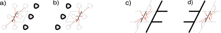
Figure 4: Discrepancy cancellation due to neighbor image sums. Each arrow represents the influence of a source density on a target segment. a) For the four upper sub-blocks of $C$, the six nearest source images (dotted) contribute to the discrepancy on the left wall $L$. b) The six nearest source images (dotted) contribute exactly the same field (suitable phased) to the right wall $(L+\textbf{e}_{1})$. The net result is that only the distant sources, shown in bold, have a non-zero effect. The same holds for all four upper sub-blocks of $C$. A rotated version applies to the lower four sub-blocks of $C$. c,d) Contributions to the sub-blocks $Q_{LL}$ and $Q_{LB}$ of $Q$. The seven indicated terms (dotted source segments) cancel in the two diagrams, leaving only the contributions from distant wall segments shown in bold. A rotated version applies to the sub-blocks $Q_{BL}$ and $Q_{BB}$.

4.2 Choice of auxiliary densities and their images

The auxiliary field $u_{\mbox{\tiny QP}}$ is determined by the choice of layer potentials on the boundary of (and outside of) $U$. We will use double and single layer densities on both the left $(L)$ and bottom $(B)$ boundaries of $U$, as well as on the other segments of the “tic-tac-toe” board in Fig. 1b. More precisely, we define the vector of unknowns $\xi$ by $\xi:=[\tau_{L};-\sigma_{L};\tau_{B};-\sigma_{B}]$, and set

$$u_{\mbox{\tiny QP}}=\!\!\!\sum_{\begin{subarray}{c}j\in\{0,1\}\\ k\in\{-1,0,1\}\end{subarray}}\!\!\!\alpha^{j}\beta^{k}\left({\cal S}_{L+j\textbf{e}_{1}+k\textbf{e}_{2}}\sigma_{L}+{\cal D}_{L+j\textbf{e}_{1}+k\textbf{e}_{2}}\tau_{L}\right)\;\;+\!\!\sum_{\begin{subarray}{c}j\in\{-1,0,1\}\\ k\in\{0,1\}\end{subarray}}\!\!\!\alpha^{j}\beta^{k}\left({\cal S}_{B+j\textbf{e}_{1}+k\textbf{e}_{2}}\sigma_{B}+{\cal D}_{B+j\textbf{e}_{1}+k\textbf{e}_{2}}\tau_{B}\right)$$ (41)

The inclusion of the image segments leads to cancellations that are numerically advantageous in the operator $Q$, just as we found that images helped with the operator $C$ in the preceding section.

We should first clarify the definition (28) of the discrepancy functions: field values should be interpreted as their limiting values on the wall approaching from inside $U$, since it is the field in $U$ that (33) and (41) represent. For example, $f:=u^{+}|_{L}-\alpha^{-1}u^{-}|_{L+\textbf{e}_{1}}$, where, as before $u^{\pm}(\textbf{x}):=\lim_{\varepsilon\to 0^{+}}u(\textbf{x}\pm\varepsilon{\bm{n}})$, and ${\bm{n}}$ is the normal at x.

Recall now that the operator $Q$ expresses the effect of the four densities in $\xi$ on the four discrepancy functions $f$, $f^{\prime}$, $g$, $g^{\prime}$. If (41) contained only the terms $j=k=0$, this would correspond to densities $\sigma_{L}$ and $\tau_{L}$ placed on $L$, and $\sigma_{B}$ and $\tau_{B}$ placed on $B$. While this is mathematically acceptable, it results in various complicated self-interactions and interactions between segments that share a common corner. This would lead to singularities in densities requiring more complicated discretization and quadrature. Although there has been significant progress in this direction (see, for example, [11, 25]), in the present context we have the luxury of including the ten additional image segments in (41), which cancel both the self and near-field corner interactions. As a result, our implementation is simpler and involves fewer degrees of freedom. The cancellation mechanism is shown in Fig. 4. The effect on $u^{+}|_{L}$ of the seven segments touching $L$, for example, cancels the effect on $u^{-}|_{L+\textbf{e}_{1}}$ of the seven segments touching $L+\textbf{e}_{1}$, leaving only ten far field contributions.

It is important to note that the local terms due to the jump relations do not cancel: e.g. a density function $\tau_{L}$ placed on $L$ contributes a term $\frac{1}{2}\tau_{L}$ to $u^{+}|_{L}$, while $\alpha\tau_{L}$ placed on $L+\textbf{e}_{1}$ contributes $-\frac{1}{2}\alpha\tau_{L}$ to $u^{-}|_{L+\textbf{e}_{1}}$. These two terms add to contribute $\tau_{L}$ to $f$. One may check in this fashion that the jump relations contribute an identity to the diagonal sub-blocks of $Q$. This yields the crucial result that $Q$ is the identity plus a compact operator, with the compact part generated by interactions at a distance greater than the size of the unit cell. After the above cancellations and simplification, we have,

$$Q=I\,+\,\begin{bmatrix}Q_{LL}&Q_{LB}\\ Q_{BL}&Q_{BB}\end{bmatrix}$$

where

$$Q_{LL} =\begin{bmatrix}\displaystyle\sum\limits_{j\in\{-1,1\},k\in\{-1,0,1\}}\!\!\!j\alpha^{j}\beta^{k}D_{L,L+j\textbf{e}_{1}+k\textbf{e}_{2}}&\qquad-\displaystyle\sum\limits_{j\in\{-1,1\},k\in\{-1,0,1\}}\!\!\!j\alpha^{j}\beta^{k}S_{L,L+j\textbf{e}_{1}+k\textbf{e}_{2}}\\ \\ \displaystyle\sum\limits_{j\in\{-1,1\},k\in\{-1,0,1\}}\!\!\!j\alpha^{j}\beta^{k}T_{L,L+j\textbf{e}_{1}+k\textbf{e}_{2}}&\qquad-\displaystyle\sum\limits_{j\in\{-1,1\},k\in\{-1,0,1\}}\!\!\!j\alpha^{j}\beta^{k}D^{\ast}_{L,L+j\textbf{e}_{1}+k\textbf{e}_{2}}\end{bmatrix}$$

$$Q_{LB} =\begin{bmatrix}\displaystyle\sum\limits_{k\in\{0,1\}}\!\beta^{k}\bigl{(}\alpha D_{L,B+\textbf{e}_{1}+k\textbf{e}_{2}}-\alpha^{-2}D_{L,B-2\textbf{e}_{1}+k\textbf{e}_{2}}\bigr{)}&\displaystyle\sum\limits_{k\in\{0,1\}}\!\beta^{k}\bigl{(}-\alpha S_{L,B+\textbf{e}_{1}+k\textbf{e}_{2}}+\alpha^{-2}S_{L,B-2\textbf{e}_{1}+k\textbf{e}_{2}}\bigr{)}\\ \\ \displaystyle\sum\limits_{k\in\{0,1\}}\!\beta^{k}\bigl{(}\alpha T_{L,B+\textbf{e}_{1}+k\textbf{e}_{2}}-\alpha^{-2}T_{L,B-2\textbf{e}_{1}+k\textbf{e}_{2}}\bigr{)}&\displaystyle\sum\limits_{k\in\{0,1\}}\!\beta^{k}\bigl{(}-\alpha D^{\ast}_{L,B+\textbf{e}_{1}+k\textbf{e}_{2}}+\alpha^{-2}D^{\ast}_{L,B-2\textbf{e}_{1}+k\textbf{e}_{2}}\bigr{)}\end{bmatrix}$$

$$Q_{BL} =\begin{bmatrix}\displaystyle\sum\limits_{j\in\{0,1\}}\!\alpha^{j}\bigl{(}\beta D_{B,L+j\textbf{e}_{1}+\textbf{e}_{2}}-\beta^{-2}D_{B,L+j\textbf{e}_{1}-2\textbf{e}_{2}}\bigr{)}&\displaystyle\sum\limits_{j\in\{0,1\}}\!\alpha^{j}\bigl{(}-\beta S_{B,L+j\textbf{e}_{1}+\textbf{e}_{2}}+\beta^{-2}S_{B,L+j\textbf{e}_{1}-2\textbf{e}_{2}}\bigr{)}\\ \\ \displaystyle\sum\limits_{j\in\{0,1\}}\!\alpha^{j}\bigl{(}\beta T_{B,L+j\textbf{e}_{1}+\textbf{e}_{2}}-\beta^{-2}T_{B,L+j\textbf{e}_{1}-2\textbf{e}_{2}}\bigr{)}&\displaystyle\sum\limits_{j\in\{0,1\}}\!\alpha^{j}\bigl{(}-\beta D^{\ast}_{B,L+j\textbf{e}_{1}+\textbf{e}_{2}}+\beta^{-2}D^{\ast}_{B,L+j\textbf{e}_{1}-2\textbf{e}_{2}}\bigr{)}\end{bmatrix}$$

$$Q_{BB} =\begin{bmatrix}\displaystyle\sum\limits_{j\in\{-1,0,1\},k\in\{-1,1\}}\!\!\!k\alpha^{j}\beta^{k}D_{B,B+j\textbf{e}_{1}+k\textbf{e}_{2}}&\displaystyle\qquad-\sum\limits_{j\in\{-1,0,1\},k\in\{-1,1\}}\!\!\!k\alpha^{j}\beta^{k}S_{B,B+j\textbf{e}_{1}+k\textbf{e}_{2}}\\ \\ \displaystyle\sum\limits_{j\in\{-1,0,1\},k\in\{-1,1\}}\!\!\!k\alpha^{j}\beta^{k}T_{B,B+j\textbf{e}_{1}+k\textbf{e}_{2}}&\displaystyle\qquad-\sum\limits_{j\in\{-1,0,1\},k\in\{-1,1\}}\!\!\!k\alpha^{j}\beta^{k}D^{\ast}_{B,B+j\textbf{e}_{1}+k\textbf{e}_{2}}\end{bmatrix}$$

Finally, we discuss the $B$ operator from (34), which describes the effect of the auxiliary densities $\xi$ on the mismatch. As with $A$, since the mismatch involves values on only a single curve ${\partial\Omega}$, there is no opportunity for cancellation. Inserting (41) into (21) we get

$$B\,=\!\! \sum_{j\in\{0,1\},k\in\{-1,0,1\}}\!\!\!\!\alpha^{j}\beta^{k}\begin{bmatrix}D_{{\partial\Omega},L+j\textbf{e}_{1}+k\textbf{e}_{2}}&-S_{{\partial\Omega},L+j\textbf{e}_{1}+k\textbf{e}_{2}}&0&0\\ T_{{\partial\Omega},L+j\textbf{e}_{1}+k\textbf{e}_{2}}&-D^{\ast}_{{\partial\Omega},L+j\textbf{e}_{1}+k\textbf{e}_{2}}&0&0\\ \end{bmatrix}\;\;+\!$$

$$\sum_{j\in\{-1,0,1\},k\in\{0,1\}}\!\!\!\!\alpha^{j}\beta^{k}\begin{bmatrix}0&0&D_{{\partial\Omega},B+j\textbf{e}_{1}+k\textbf{e}_{2}}&-S_{{\partial\Omega},B+j\textbf{e}_{1}+k\textbf{e}_{2}}\\ 0&0&T_{{\partial\Omega},B+j\textbf{e}_{1}+k\textbf{e}_{2}}&-D^{\ast}_{{\partial\Omega},B+j\textbf{e}_{1}+k\textbf{e}_{2}}\\ \end{bmatrix}$$ (42)

Summarizing the above, $E$ is a compact perturbation of the identity. Its blocks $C$ and $Q$ involve interaction distances greater than the unit cell size. Its block $A$ involves distances controlled by the shape of the inclusion and its nearest approach to its neighboring images. Its block $B$ involves distances determined by the nearest approach of ${\partial\Omega}$ to $\partial U$.

4.3 Numerical implementation and discretization of $B$

We discretize the four blocks of the integral operator $E$ in (34) to give the matrix $\tilde{E}\in\mathbb{C}^{(2N+4M)\times(2N+4M)}$ as follows. We sample the densities on ${\partial\Omega}$ at equispaced points with respect to the given definition of the curve, as in Section 3.1. We sample the densities on the walls $L$ and $B$ at $M$ standard Gaussian nodes, as in Section 3.2. $A$ is then discretized in the same way as $A_{{\mbox{\tiny\rm QP}}}$ in Section 3.1 with a mix of the periodic trapezoidal rule and Kress’ singular quadratures for the self-interaction of ${\partial\Omega}$. The (Nyström) method (22) may be used for the off-diagonal block $C$, and also for the wall’s self-interaction $Q$. No special singular quadratures are needed in $Q$, due to the cancellations discussed above.

The $B$ operator (42) involves computing the field due to source densities on walls $L$ and $B$ (and their images shown in Fig. 1b) at targets on ${\partial\Omega}$. When the distance from the inclusion to boundary $\operatorname{dist}({\partial\Omega},\partial U)$ is large, the plain Nyström method may be used to construct the discretized matrix $\hat{B}$. We will refer to this as discretization method B1. With nodes $\textbf{y}_{m}$ and weights $w_{m}$ on wall $L$, and nodes $\textbf{x}_{j}$ on ${\partial\Omega}$, for example, the term $S_{{\partial\Omega},L}$ in the (1,2)-block of (42) becomes the matrix $\hat{S}\in\mathbb{C}^{N\times M}$ with elements $\hat{S}_{jm}=\frac{i}{4}H^{(1)}_{0}(\omega|\textbf{x}_{j}-\textbf{y}_{m}|)w_{m}$.

When $\operatorname{dist}({\partial\Omega},\partial U)$ becomes small, of course, the convergence rate of method B1 will become unacceptably poor. However, by construction, for a Bloch eigenfunction the field (41) generated by the wall densities in $\xi$ has no singularities in the $3\times 3$ neighboring block of unit cells. Hence these densities remain smooth, poor convergence being merely due to inaccurate evaluation of their field close to the walls. This leaves room for a large number of options:

1. For the rows of $\hat{B}$ corresponding to target points on ${\partial\Omega}$ that are distance $d_{0}$ or closer to ${\partial U}$, use adaptive Gauss-Kronrod quadrature with integrand given by the product of the kernel function and the Lagrange polynomial interpolant [32, Sec. 8.1] for the density at the $M$ quadrature points. $d_{0}$ is some $O(1)$ constant. For the other rows, use method B1.

2. Project onto an order-$L$ cylindrical $J$-expansion at the origin. This is done by computing a representation (27) for each of the point monopole or dipole sources in the quadrature approximation to the source densities on the walls, and then evaluating this at the target quadrature points on ${\partial\Omega}$ to fill the elements of $\hat{B}$. The example term discussed for B1 gives $\hat{S}=RP$, where the “source-to-local” matrix $P\in\mathbb{C}^{(2L+1)\times M}$ has elements

   $$P_{lm}=\frac{i}{4}H^{(1)}_{l}(\omega|\textbf{y}_{m}|)e^{-il\theta_{m}}w_{m}$$

   and converts single layer density values to $J$-expansion coefficients. This follows from Graf’s addition formula [1, Eq. 9.1.79]. The expansion matrix $R\in\mathbb{C}^{N\times(2L+1)}$ has elements $R_{jl}=J_{l}(\omega|\textbf{x}_{j}|)e^{il\phi_{j}}$. In the above $\theta_{m},\phi_{j}$ are polar angles of points $\textbf{y}_{m},\textbf{x}_{j}$ respectively. Similar formulae apply for double layers and evaluation of derivatives. To reduce dynamic range (hence roundoff error) we in fact scale the $J$-expansion by the factors $\rho_{l}$ of Section 3.2 (this does not change the mathematical definition of $\hat{S}$.)

3. Use a more sophisticated quadrature approach, such as those of [5, 26, 37].

Methods B2-B4 evaluate $u_{\mbox{\tiny QP}}$ due to a spectral interpolant of the discretized wall densities, with an accuracy that persists up to the boundary of $U$. Note that this does not increase the number $M$ of degrees of freedom associated with each such density. Since the underlying density is smooth (in fact analytic), the convergence rate is high and we are able to keep $M$ very modest.

We have implemented methods B1, B2 and B3. We use the quadrature weights to scale the matrix $\hat{E}$ to give $\tilde{E}$ in an analogous fashion to (26), so that singular values of $\tilde{E}$ approximate those of $E$.

Finally, there are many possible ways to locate parameter values $(\omega,a,b)$ where $\tilde{E}$ is singular. In this paper, we will simply plot its smallest singular value $\sigma_{\mbox{\tiny min}}(\tilde{E})$ vs the Bloch parameters, as in Section 3.

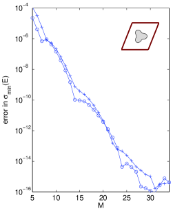
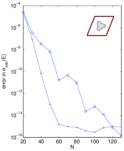
a) b) c)

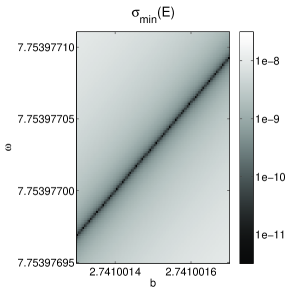
Figure 5: Convergence of new periodizing scheme using auxilliary densities (described in Section 4), using method B1, for the same geometry and parameters as in Fig. 2a. The meaning of the two curves is also the same as in the earlier figure. a) Absolute error in $\sigma_{\mbox{\tiny min}}(\tilde{E})$ vs $M$ the number of nodes on each unit cell wall, for fixed $N=70$ nodes on ${\partial\Omega}$. b) Same as a) except convergence vs $N$, for fixed $M=30$. c) Same as Fig. 3b but using the new scheme: note the absence of pollution by the empty band structure.

5 Results of proposed scheme

We first test the convergence of the new scheme for the same small inclusion used in Section 3, with the simplest discretization method for $B$, namely B1. As before, we test two Bloch parameter $b$ values, one which is far from an eigenvalue, and one of which is guaranteed to be an eigenvalue according to Theorem 4. Fixing $N=70$, which was found in Section 3.1 to be fully converged when at an eigenvalue, we first vary $M$, the number of nodes per unit cell wall. Fig. 5a shows the convergence of the minimum singular value of the discretized matrix $\tilde{E}$ to its converged value (when far from an eigenvalue), or to zero (when at an eigenvalue). The convergence is spectral, and in both cases full machine accuracy is reached at $M=30$. (For $N>70$ the results are unchanged.) Thus for a matrix of order $2N+4M=260$, we are able to locate the desired band structure with relative error around $10^{-15}$ in the Bloch parameters $(a,b)$. Filling such a matrix takes around 0.45 sec and computing the complex SVD around 0.15 sec. Furthermore, by storing coefficient matrices in the expansion $\tilde{E}=\sum_{-1\leq j,k\leq 2}\alpha^{j}\beta^{k}\tilde{E}^{(j,k)}$ at fixed $\omega$, we can fill $\tilde{E}$ for new $a,b$ values in 0.05 sec.

Fig. 5b shows that, with $M$ in the new quasi-periodizing scheme sufficient to yield machine precision, the error convergence rate with respect to $N$ is the same as that of the old scheme. Fig. 5c demonstrates the robustness of the scheme, by plotting the smallest singular value over the same region of parameter space as Fig. 3b. Notice that the location of the desired band structure (black line) is unchanged, but that the divergent behavior near the empty resonant band structure has entirely vanished.

 

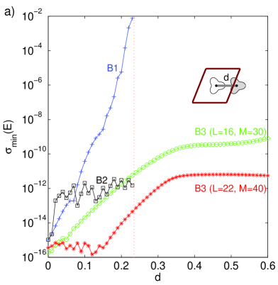
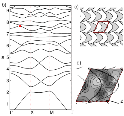
Figure 6: a) Dependence of $\sigma_{\mbox{\tiny min}}(\tilde{E})$ on $x$-translation distance $d$ of ${\partial\Omega}$ relative to the system of Fig. 2a, for fixed $N=70$, and $M=30$. The vertical line shows where ${\partial\Omega}$ starts to touch ${\partial U}$. $B$ is discretized as follows: method B1 (+ symbols), method B2 with $d_{0}=0.2$ ($\square$ symbols), method B3 with $L=16$ ($\circ$ symbols), method B3 with $L=22$ and $M=40$ ($\ast$ symbols). Inset shows unit cell and inclusion at $d=0.6$. b) Band structure for crescent-shaped photonic crystal shown in c), index $n=2$, shape $(0.265\cos 2\pi t+0.318\cos 4\pi t,0.53\sin 2\pi t)$, $0\leq t<1$, unit cell $\textbf{e}_{1}=(1,0)$, $\textbf{e}_{2}=(0.45,1)$. A tour $\Gamma XM\Gamma$ of the Brillouin zone is shown, where $\Gamma$ is $(a,b)=(0,0)$, $X$ is $(\pi,0)$, and $M$ is $(\pi,\pi)$. d) Contours of the Bloch mode Re$[u]$ with parameters shown by the dot on the band diagram.

5.1 Inclusions approaching and intersecting the unit cell wall

Given a crystal of inclusions, it may be impossible to choose a parallelogram unit cell $U$ whose boundary does not come close to or even intersect ${\partial\Omega}$. Although this is not an issue for the scheme of Section 3, for the new scheme which relies on ${\partial U}$ it is a potential problem.

We first show that, as expected, with method B1 the error performance deteriorates exponentially as ${\partial\Omega}$ approaches ${\partial U}$. In Fig. 6a we plot the minimum singular value at a Bloch eigenvalue, as a function of distance $d$ that the inclusion has been translated in the $x$ direction (translation does not affect the Bloch eigenvalue.) Numerical parameters $N$ and $M$ are held fixed. The logarithm of the error grows roughly linearly with $d$ and reaches $O(1)$ for $\operatorname{dist}({\partial\Omega},{\partial U})=0$, indicated by the dotted vertical line at around $d=0.23$. Method B2, also shown in Fig. 6a, uses adaptive quadrature for accurate evaluation of $u_{\mbox{\tiny QP}}$ in all of $U$. For very small $d$, the inclusion is still centrally located (far from the wall) and B2 is identical to B1, with an error of $10^{-15}$. The error is around $10^{-12}$ as one approaches the wall (more or less independent of $d$), limited by the accuracy of quadgk. This proves that the deterioration seen with B1 is associated with the $B$ operator block, and can be remedied merely by careful discretization of $B$ without increasing the matrix size. We did not bother continuing the computation with B1 or B2 after the inclusion crosses the wall; here they fail because (41), as constructed, represents $u_{\mbox{\tiny QP}}$ only inside $U$ (jump relations cause the values outside $U$ to be different). We note that to use B1 or B2 correctly, one would have to wrap the boundary points outside $U$ back into the cell, evaluate at the wrapped point, and correct for phase. Method B2 is not very useful in practice since the call to a black box adaptive quadrature routine causes the matrix fill time to increase to 55 sec.

Finally we use method B3 with $L=16,M=30$ and with $L=22,M=40$. In the first case, errors grow slowly to around $10^{-12}$ as $\operatorname{dist}({\partial\Omega},{\partial U})$ reaches zero, and then continue to grow slowly to a plateau at around $10^{-9}$, even though most of ${\partial\Omega}$ now falls outside of the unit cell. The cost of B3 is not much more than B1, taking 0.7 sec to fill $\tilde{E}$. Note that the $J$-expansion used to represent $u_{\mbox{\tiny QP}}$ has effectively carried out analytic continuation beyond $U$. This is stable because our image structure has pushed the singularities out beyond the nearest image cells. It is perhaps worth observing that some care must be taken in setting $L$. With $M=30$, increasing $L$ above 16 would worsen errors (not shown). The reason is that the coefficients $|l|>16$ involve more oscillatory integrands which are not resolved by $M=30$ points. Increasing $M$ to 40 permits increased precision with $L=22$, as seen in Fig. 6a.

There is another potential pitfall with method B3 as implemented; if both $L$ and $d$ get larger, there may arise singular values of $\tilde{E}$ which become exponentially small, associated with highly oscillatory non-physical densities on the farthest part of ${\partial\Omega}$. For illustration, with $L=16$ and $d=0.6$, the second-smallest singular value is $10^{-4}$; with $L=22$ the second smallest singular value shrinks to $10^{-6}$. (When $d=0$, the second smallest singular value is $10^{-1}$.) This is troublesome for eigenvalue search methods that track $\sigma_{\mbox{\tiny min}}(\tilde{E})$ vs Bloch parameters, since the desired minima will be obscured by these spurious small singular values everywhere except in a small neighborhood of the desired band structure. We will discuss search methods less sensitive to this problem in a future paper. For now the lesson is that, when parts of an inclusion extend far beyond $U$, there is a price to pay for making use of analytic continuation.

5.2 Application to band structure

We compute the band structure of a more difficult crystal in Fig. 6b. $\Omega$ is far from circular, hence simple multipole methods [23] would not be accurate. The closest approach to its neighbors is only 0.06, so that $N=150$ points are needed in discretizing the inclusion boundary. Note that any parallelogram unit cell must intersect ${\partial\Omega}$, so the method of [49] cannot be used without modification. We use method B3 with $M=35$ and $L=18$. As illustrated before in Fig. 2b, the minimum values of $\sigma_{\mbox{\tiny min}}(\tilde{E})$ on the band structure indicate the size of the errors in the Bloch parameters found. By this measure, sampling 100 random points on the first 15 bands, we find a median error of $3\times 10^{-10}$ and a maximum $1.6\times 10^{-9}$. 1.7 sec were required to fill the matrix $\tilde{E}$ of order $440$ once for a given $\omega,a,b$ (and 0.13 sec for subsequent values of $a,b$). The SVD required 0.7 sec for a matrix of this size. We located the band structure using $8000$ such evaluations and a specialized search algorithm, which we will describe in a forthcoming paper. The search algorithm is also accelerated by computing the determinant of $\tilde{E}$ rather than the SVD, at a cost of 0.1 sec for each matrix. The total CPU time required was 35 minutes.

Fig. 6d shows a single Bloch mode on the 11th band for this crescent-shaped crystal. This took 16 sec to evaluate on a $100\times 100$ grid over $U$ using (33), and the $J$-expansion for (41) (with no fast multipole acceleration).

6 Conclusions

We have presented two algorithms for locating the band structure of a two-dimensional photonic crystal, in the $z$-invariant Maxwell setting. The first (Section 3) uses the quasi-periodic Green’s function. Theorem 4 guarantees the success of this method (no spurious or missed modes) as long as the band structure for the empty unit cell is avoided, where we have shown that the method fails. The second method (Section 4) introduces a small number of additional degrees of freedom on the walls to represent the periodizing part of the field: numerical evidence suggests that it is immune to breakdown for any Bloch parameters (Conjecture 7). The two schemes are connected by the following observation.

Remark 8

Computing the Schur complement formula for the operator system (34) recovers the quasi-periodic Green’s function approach described by (20). In particular,

$$A_{{\mbox{\tiny\rm QP}}}=A-BQ^{-1}C.$$

The quasi-periodic Green’s function approach fails when $Q$ becomes singular and $A_{{\mbox{\tiny\rm QP}}}$ blows up. The full system (34), on the other hand, remains well-behaved.

We have shown spectral convergence for both schemes, achieving close to machine precision accuracy on simple crystals using only a few hundred degrees of freedom, hence CPU times of less than 1 sec for testing at a single parameter set $(\omega,a,b)$. In the new scheme we have shown (method B3) how to handle the passage of the inclusion through the unit cell boundary, without much sacrifice in accuracy, without much extra numerical effort, and with no bookkeeping needed to determine which points of ${\partial\Omega}$ lie in $U$. The latter is convenient for larger-scale or three-dimensional (3D) computations if existing scattering codes are to be used to fill the $A$ operator block. Other ways to handle this intersection problem exist, such as a variant of B2 which wraps points on ${\partial\Omega}$ back into $U$, with which we have preliminary success.

We have not discussed the methods we use for the nonlinear eigenvalue problem, due to space constraints. The scheme of Yuan et al [49] uses a quadratic eigenvalue problem, and factorizes the scattering matrix of the inclusion at each $\omega$, hence may be faster than our scheme for small systems. However, moving to large-scale systems with more than $10^{4}$ degrees of freedom, such a factorization would be impractical compared to an iterative version of our scheme.

Some generalizations of what we present are straightforward, such as multiple inclusions per unit cell, non-simply connected inclusions, or inclusions with corners (using quadrature rules such as [11, 25]). There exist regimes, however, that would require some modification. These include two phase dielectrics one or more of which are connected through the bulk (sometimes called bicontinuous), and unit cells which are highly skew or have large aspect ratios.

Our new representation for quasi-periodic fields can also be used for scattering calculations from periodic one-dimensional arrays of inclusions in 2D and one or two-dimensional arrays in 3D. Because we rely entirely on the free-space Green’s function, it should be straightforward to create quasi-periodic solvers from existing scattering codes. We will describe such solvers at a later date.

Appendix A Proof of Theorem 4

Recall the Green’s representation formulae [16, Sec. 3.2]. If $u$ satisfies $(\Delta+\omega^{2})u=0$ in $\Omega$, recalling that $u^{-}$ and $u^{-}_{n}$ signify limits on ${\partial\Omega}$ approaching from the inside, and the normal always points outwards from $\Omega$, then

$$-{\cal S}^{(\omega)}u^{-}_{n}+{\cal D}^{(\omega)}u^{-}\;=\;\left\{\begin{array}[]{ll}-u&\mbox{in }\Omega\\ 0&\mbox{in }\mathbb{R}^{2}\setminus\overline{\Omega}\end{array}\right.$$ (43)

The exterior representation has the opposite sign: let $u$ satisfy $(\Delta+\omega^{2})u=0$ in $\mathbb{R}^{2}\setminus\overline{\Omega}$ and the Sommerfeld radiation condition, that is,

$$\frac{\partial u}{\partial r}-i\omega u=o(r^{-1/2}),\qquad r:=|\textbf{x}|\to\infty$$ (44)

holds uniformly with respect to direction $\textbf{x}/r$. Then,

$$-{\cal S}^{(\omega)}u^{+}_{n}+{\cal D}^{(\omega)}u^{+}\;=\;\left\{\begin{array}[]{ll}0&\mbox{in }\Omega\\ u&\mbox{in }\mathbb{R}^{2}\setminus\overline{\Omega}\end{array}\right.$$ (45)

We will need the following quasi-periodic analogues.

Lemma 9

Let $u$ satisfy $(\Delta+\omega^{2})u=0$ in $\Omega$, and $\overline{\Omega}\subset U$, Then for each Bloch phase $(\alpha,\beta)$,

$$-{\cal S}^{(\omega)}_{\mbox{\tiny\rm QP}}u^{-}_{n}+{\cal D}^{(\omega)}_{\mbox{\tiny\rm QP}}u^{-}\;=\;\left\{\begin{array}[]{ll}-u&\mbox{\rm in }\Omega\\ 0&\mbox{\rm in }U\setminus\overline{\Omega}\end{array}\right.$$ (46)

Proof: Write $G_{{\mbox{\tiny\rm QP}}}$ using (11) and notice that each term other than $(m,n)=(0,0)$ contributes zero. This is because all points in $U$ lie outside each closed curve ${\partial\Omega}-m\textbf{e}_{1}-n\textbf{e}_{2}$, and we may apply the second (extinction) case of (43) to show that they have no effect in $U$. $\square$

Lemma 10

Let $u$ satisfy $(\Delta+\omega^{2})u=0$ in $U\setminus\overline{\Omega}$ and quasi-periodicity (6)-(9), and $\overline{\Omega}\subset U$. Then

$$-{\cal S}^{(\omega)}_{\mbox{\tiny\rm QP}}u^{+}_{n}+{\cal D}^{(\omega)}_{\mbox{\tiny\rm QP}}u^{+}\;=\;\left\{\begin{array}[]{ll}0&\mbox{\rm in }\Omega\\ u&\mbox{\rm in }U\setminus\overline{\Omega}\end{array}\right.$$ (47)

Proof: We follow the usual method of proof [16, Thm. 3.3] but with the quasi-periodicity condition playing the role of the radiation condition. Apply Green’s 2nd identity to the functions $u$ and $G_{{\mbox{\tiny\rm QP}}}(\textbf{x},\cdot)$ in the domain $U\setminus\overline{\Omega}$ if $\textbf{x}\in\Omega$, or the domain $\{\textbf{y}\in U\setminus\overline{\Omega}:|\textbf{x}-\textbf{y}|>\varepsilon\}$ if $\textbf{x}\in U\setminus\overline{\Omega}$. In the latter case the limit $\varepsilon\to 0$ is taken, and (11) shows that only the $(m,n)=(0,0)$ term contributes to the limit of the integral over the sphere of radius $\varepsilon$. In both cases the boundary integrals contain the term

$$\int_{\partial U}\frac{\partial G_{{\mbox{\tiny\rm QP}}}}{\partial n_{\textbf{y}}}(\textbf{x},\textbf{y})u(\textbf{y})-G_{{\mbox{\tiny\rm QP}}}(\textbf{x},\textbf{y})u_{n}(\textbf{y})\;ds_{\textbf{y}}~{},$$ (48)

which vanishes by cancellation on opposing walls, since $u$ is quasi-periodic with phases $(\alpha,\beta)$, but $G_{{\mbox{\tiny\rm QP}}}(\textbf{x},\cdot)$ is anti-quasiperiodic, i.e. quasi-periodic with phases $(\alpha^{-1},\beta^{-1})$. $\square$

Turning now to Theorem 4, to prove the if part, we show that whenever the operator has a nontrivial nullspace, a Bloch eigenfunction $u$ may be constructed, i.e. a solution to (2)-(9) that we must take care to show is nontrivial. Let $\eta=[\tau;-\sigma]\neq 0$ be a nontrivial density such that $A_{{\mbox{\tiny\rm QP}}}\eta=0$. Immediately we have that the resulting field $u$ given by (15) satisfies (2)-(9). We now define a complementary field over the whole plane minus ${\partial\Omega}$,

$$v\;=\;\left\{\begin{array}[]{ll}{\cal S}^{(\omega)}_{\mbox{\tiny QP}}\sigma+{\cal D}^{(\omega)}_{\mbox{\tiny QP}}\tau&\mbox{in }\Omega\\ -{\cal S}^{(n\omega)}\sigma-{\cal D}^{(n\omega)}\tau&\mbox{in }\mathbb{R}^{2}\setminus\overline{\Omega}\end{array}\right.$$ (49)

Suppose $u\equiv 0$. Then $u^{-}=u_{n}^{-}=0$ and by the jump relations for ${\cal S}^{(n\omega)}\sigma+{\cal D}^{(n\omega)}\tau$ we get $v^{+}=-\tau$ and $v_{n}^{+}=\sigma$. Similarly, since $u^{+}=u_{n}^{+}=0$ by the jump relations for ${\cal S}^{(\omega)}_{\mbox{\tiny QP}}\sigma+{\cal D}^{(\omega)}_{\mbox{\tiny QP}}\tau$ we get $v^{-}=-\tau$ and $v_{n}^{-}=\sigma$. It is easy to check that $v$ solves the (swapped-wavenumber) transmission problem,

$$(\Delta+\omega^{2})v = 0\qquad\mbox{in }\Omega$$ (50)

$$(\Delta+n^{2}\omega^{2})v = 0\qquad\mbox{in }\mathbb{R}^{2}\setminus\overline{\Omega}$$ (51)

$$\frac{\partial v}{\partial r}-in\omega v = o(r^{-1/2}),\qquad r\to\infty,\mbox{ uniformly in direction}$$ (52)

$$v^{+}-v^{-} = h$$ (53)

$$v_{n}^{+}-v_{n}^{-} = h^{\prime}$$ (54)

with homogeneous boundary discontinuity data $h=h^{\prime}=0$. By uniqueness for this problem [16, Thm. 3.40] we get that $v\equiv 0$ in $\mathbb{R}^{2}$, from which the jump relations back to $u$ imply $\sigma=\tau=0$, which contradicts our assumption of nontrivial density. Thus $u$ is a Bloch eigenfunction.

To prove the only if part we show that, given the existence of a Bloch eigenfunction, we may exhibit a (nontrivial) density $\eta$ such that $A_{{\mbox{\tiny\rm QP}}}\eta=0$. Let $w$ be a Bloch eigenfunction with eigenvalue $(\omega,a,b)$. Then let $v$ solve (50)-(54) with the inhomogeneous data $h=-2w|_{\partial\Omega}$ and $h^{\prime}=-2w_{n}|_{\partial\Omega}$. (Note that $w$ obeys continuity (4), hence $w|_{\partial\Omega}=w^{+}=w^{-}$ and $w_{n}|_{\partial\Omega}=w^{+}_{n}=w^{-}_{n}$). By [16, Thm. 3.41] we know that a unique solution exists. We now claim that the densities

$$\sigma = w_{n}|_{\partial\Omega}+v_{n}^{+}$$ (55)

$$\tau = -w|_{\partial\Omega}-v^{+}$$ (56)

generate precisely the eigenfunction $w$, i.e. the representation $u$ of (15) obeys $u\equiv w$ in $U$. We show this by substituting the densities into (15), then applying (43) and (45) in $\Omega$, and Lemma 47 in $U\setminus\overline{\Omega}$:

$$u = \left\{\begin{array}[]{ll}{\cal S}^{(n\omega)}w_{n}|_{\partial\Omega}-{\cal D}^{(n\omega)}w|_{\partial\Omega}\;\;+\;\;{\cal S}^{(n\omega)}v_{n}^{+}-{\cal D}^{(n\omega)}v^{+}&\mbox{in }\Omega\\ {\cal S}^{(\omega)}_{\mbox{\tiny QP}}w_{n}|_{\partial\Omega}-{\cal D}^{(\omega)}_{\mbox{\tiny QP}}w|_{\partial\Omega}\;\;+\;\;{\cal S}^{(\omega)}_{\mbox{\tiny QP}}v_{n}^{+}-{\cal D}^{(\omega)}_{\mbox{\tiny QP}}v^{+}&\mbox{in }U\setminus\overline{\Omega}\end{array}\right.$$ (59)

$$= \left\{\begin{array}[]{ll}w&\mbox{in }\Omega\\ -w\;\;+\;\;{\cal S}^{(\omega)}_{\mbox{\tiny QP}}v_{n}^{+}-{\cal D}^{(\omega)}_{\mbox{\tiny QP}}v^{+}&\mbox{in }U\setminus\overline{\Omega}\end{array}\right.$$ (62)

On the remaining term, we use $v$’s known jumps $h$ and $h^{\prime}$ to get

$${\cal S}^{(\omega)}_{\mbox{\tiny QP}}v_{n}^{+}-{\cal D}^{(\omega)}_{\mbox{\tiny QP}}v^{+} = {\cal S}^{(\omega)}_{\mbox{\tiny QP}}v_{n}^{-}-{\cal D}^{(\omega)}_{\mbox{\tiny QP}}v^{-}-2{\cal S}^{(\omega)}_{\mbox{\tiny QP}}w_{n}|_{\partial\Omega}+2{\cal D}^{(\omega)}_{\mbox{\tiny QP}}w|_{\partial\Omega}$$

$$= -2w$$

where we applied Lemma 46 to the first pair, and Lemma 47 to the second as before. Substituting this above shows that $u\equiv w$ in $U$. Since $w$ has zero mismatch, the density vector $\eta:=[\tau;-\sigma]$ satisfies $A_{{\mbox{\tiny\rm QP}}}\eta=0$. Finally, $\eta$ must be nontrivial since $\eta=0$ would imply $u\equiv 0$ by (15) which contradicts it being equal to the eigenfunction $w$. $\square$

We close with a couple of remarks about the proof. Barring a sign, $v$ in (49) is the extension of $u$’s representation (15) into its nonphysical regions, a trick originating, in the homogeneous context, with the proof in [16, Thm. 3.41]. Because (15) uses $G_{{\mbox{\tiny\rm QP}}}$ outside, but $G$ inside, the complementary problem is a nonperiodic transmission problem, which has known existence and uniqueness. The related analysis of [45] uses $G_{{\mbox{\tiny\rm QP}}}$ both inside and outside. This results in a periodic problem as the complementary problem, and it is not so clear that one can eliminate the possibility of spurious modes.

References

- [1] M. Abramowitz, I. A. Stegun, Handbook of Mathematical Functions with Formulas, Graphs, and Mathematical Tables, 10th ed., Dover, New York, 1964.
- [2] B. K. Alpert, Hybrid Gauss-trapezoidal quadrature rules, SIAM J. Sci. Comput. 20 (1999) 1551–1584.
- [3] W. Axmann, P. Kuchment, An efficient finite element method for computing spectra of photonic and acoustic band-gap materials, J. Comput. Phys. 150 (1999) 468–481.
- [4] A. H. Barnett, T. Betcke, Stability and convergence of the Method of Fundamental Solutions for Helmholtz problems on analytic domains, J. Comput. Phys. 227 (2008) 7003–7026.
- [5] J. Beale, M.-C. Lai, A method for computing nearly singular integrals, SIAM J. Numer. Anal. 38 (2001) 1902–1925.
- [6] C. L. Berman, L. Greengard, A renormalization method for the evaluation of lattice sums, J. Math. Phys. 35 (1994) 6036–6048.
- [7] P. Bermel, C. Luo, L. Zeng, L. C. Kimerling, J. D. Joannopoulos, Improving thin-film crystalline silicon solar cell efficiencies with photonic crystals, Opt. Express 15 (25) (2007) 16986–17000.
- [8] T. Betcke, Computations of eigenfunctions of planar regions, Ph.D. thesis, Oxford University, UK (2005).
- [9] G. Beylkin, C. Kurcz, L. Monzón, Fast algorithms for Helmholtz Green’s functions, Proc. R. Soc. A 464 (2008) 3301–3326.
- [10] L. C. Botten, R. C. McPhedran, N. A. Nicorovici, A. A. Asatryan, C. M. de Sterke, P. A. Robinson, K. Busch, G. H. Smith, T. N. Langtry, Rayleigh multipole methods for photonic crystal calculations, Progress in Electromagnetics Research 41 (2003) 21–60.
- [11] J. Bremer, V. Rokhlin, I. Sammis, Universal quadratures for boundary integral equations on two-dimensional domains with corners, Yale University Department of Computer Science Technical Report 1420.
- [12] H. Cheng, W. Y. Crutchfield, Z. Gimbutas, G. L., F. Ethridge, J. Huang, V. Rokhlin, N. Yarvin, J. Zhao, A wideband fast multipole method for the Helmholtz equation in three dimensions, J. Comput. Phys. 216 (2006) 300–325.
- [13] H. Cheng, W. Y. Crutchfield, Z. Gimbutas, G. L., J. Huang, V. Rokhlin, N. Yarvin, J. Zhao, Remarks on the implementation of the wideband FMM for the Helmholtz equation in two dimensions, vol. 408 of Contemp. Math., Amer. Math. Soc., Providence, RI, 2006, pp. 99–110.
- [14] W. C. Chew, J. M. Jin, E. Michielssen, J. Song, Fast and Efficient Algorithms in Computational Electromagnetics, Artech House, Boston, MA, 2001.
- [15] S. K. Chin, N. A. Nicorovici, R. C. McPhedran, Green’s function and lattice sums for electromagnetic scattering by a square array of cylinders, Phys. Rev. E 49 (5) (1994) 4590–4602.
- [16] D. Colton, R. Kress, Integral equation methods in scattering theory, Wiley, 1983.
- [17] W. Crutchfield, H. Cheng, L. Greengard, Sensitivity analysis of photonic crystal fiber, Opt. Express 12 (2004) 4220–4226.
- [18] A. Dienstfrey, F. Hang, J. Huang, Lattice sums and the two-dimensional, periodic Green’s function for the Helmholtz equation, Proc. R. Soc. Lond. A 457 (2001) 67–85.
- [19] D. C. Dobson, An efficient method for band structure calculations in 2d photonic crystals, J. Comput. Phys. 149 (1999) 363–376.
- [20] K. Dossou, M. Byrne, L. C. Botten, Finite element computation of grating scattering matrices and application to photonic crystal band calculations, J. Comput. Phys. 219 (2006) 120–143.
- [21] S. Fan, P. R. Villeneuve, J. D. Joannopoulos, H. A. Haus, Channel drop filters in a photonic crystal, Opt. Express 3 (1998) 4–11.
- [22] R. B. Guenther, J. W. Lee, Partial differential equations of mathematical physics and integral equations, Prentice Hall, Englewood Cliffs, New Jersey, 1988.
- [23] C. Hafner, The Generalized Multipole Technique for Computational Electromagnetics, Artech House Books, Boston, 1990.
- [24] J. Helsing, Integral equation methods for elliptic problems with boundary conditions of mixed type, J. Comput. Phys. 228 (2009) 8892–8907.
- [25] J. Helsing, R. Ojala, Corner singularities for elliptic problems: Integral equations, graded meshes, quadrature, and compressed inverse preconditioning, J. Comput. Phys. 227 (2008) 8820–8840.
- [26] J. Helsing, R. Ojala, On the evaluation of layer potentials close to their sources, J. Comput. Phys. 227 (2008) 2899–2921.
- [27] J. D. Jackson, Classical Electrodynamics, 3rd ed., Wiley, 1998.
- [28] J. D. Joannopoulos, S. G. Johnson, R. D. Meade, J. N. Winn, Photonic Crystals: Molding the Flow of Light, 2nd ed., Princeton Univ. Press, Princeton, NJ, 2008.
- [29] S. G. Johnson, J. D. Joannopoulos, Block-iterative frequency-domain methods for Maxwell’s equations in a planewave basis, Opt. Express 8 (3) (2001) 173–190.
- [30] S. Kapur, V. Rokhlin, High-order corrected trapezoidal quadrature rules for singular functions, SIAM J. Numer. Anal. 34 (1997) 1331–1356.
- [31] R. Kress, Boundary integral equations in time-harmonic acoustic scattering, Mathl. Comput. Modelling 15 (1991) 229–243.
- [32] R. Kress, Numerical Analysis, Graduate Texts in Mathematics #181, Springer-Verlag, 1998.
- [33] R. Kress, Linear Integral Equations, vol. 82 of Applied Mathematical Sciences, 2nd ed., Springer, 1999.
- [34] K. M. Leung, Y. Qiu, Multiple-scattering calculation of the two-dimensional photonic band structure, Phys. Rev. B 48 (11) (1993) 7767–7771.
- [35] C. M. Linton, I. Thompson, Resonant effects in scattering by periodic arrays, Wave Motion 44 (2007) 165–175.
- [36] N. M. Litchinitser, V. M. Shalaev, Photonic metamaterials, Laser Phys. Lett. 5 (6) (2008) 411–420.
- [37] A. Mayo, Fast high order accurate solution of laplace’s equation on irregular regions, SIAM J. Sci. Stat. Comput. 6 (1985) 144–157.
- [38] R. C. McPhedran, N. A. Nicorovici, L. C. Botten, K. A. Grubits, Lattice sums for gratings and arrays, J. Math. Phys. 41 (2000) 7808–7816.
- [39] M. Mitrea, Boundary value problems and Hardy spaces associated to the Helmholtz equation in Lipschitz domains, J. Math. Anal. Appl. 202 (1996) 819–842.
- [40] A. Moroz, Exponentially convergent lattice sums, Opt. Lett. 26 (2001) 1119–21.
- [41] P. Morse, H. Feshbach, Methods of theoretical physics, volume 2, McGraw-Hill, 1953.
- [42] Y. Otani, N. Nishimura, A periodic FMM for Maxwell’s equations in 3d and its applications to problems related to photonic crystals, J. Comput. Phys. 227 (2008) 4630–52.
- [43] D. Pissoort, E. Michielssen, F. Olyslager, D. D. Zutter, Fast analysis of 2D electromagnetic crystal devices using a periodic green function approach, Journal of lightwave technology 23 (7) (2005) 2294–2308.
- [44] V. Rokhlin, Solution of acoustic scattering problems by means of second kind integral equations, Wave Motion 5 (1983) 257–272.
- [45] S. Shipman, S. Venakides, Resonance and bound states in photonic crystal slabs, SIAM J. Appl. Math. 64 (2003) 322–342.
- [46] J. Smajic, C. Hafner, D. Erni, Automatic calculation of band diagrams of photonic crystals using the Multiple Multipole Method, Appl. Comput. Electromag. Soc. J. 18 (2003) 172–180.
- [47] A. Spence, C. Poulton, Photonic band structure calculations using nonlinear eigenvalue techniques, J. Comput. Phys. 204 (2005) 65–81.
- [48] E. Yablonovitch, Photonic band-gap structures, J. Opt. Soc. Am. B 10 (1993) 283–295.
- [49] J. Yuan, Y. Y. Lu, X. Antoine, Modeling photonic crystals by boundary integral equations and Dirichlet-to-Neumann maps, J. Comput. Phys. 227 (2008) 4617–4629.