Compensating the Noise of a Communication Channel
via Asymmetric Encoding of Quantum Information

Abstract

An asymmetric preparation of the quantum states sent through a noisy channel can enable a new way to monitor and actively compensate the channel noise. The paradigm of such an asymmetric treatment of quantum information is the Bennett 1992 protocol, in which the ratio between conclusive and inconclusive counts is in direct connection with the channel noise. Using this protocol as a guiding example, we show how to correct the phase drift of a communication channel without using reference pulses, interruptions of the quantum transmission or public data exchanges.

In recent years the field of Quantum Key Distribution (QKD) GRT+02 has reached such a high degree of technical perfection that the emergence of unexplored directions in one of its oldest protocols, the Bennett 1992 B92 , is somewhat surprising. The Bennett 1992 (B92) protocol is based on only two quantum states, $|\varphi_{0}\rangle$ and $|\varphi_{1}\rangle$, strictly nonorthogonal, to which are associated the two values of the logical bit communicated by the transmitter (Alice) to the receiver (Bob) B92 . This simple structure is one of the main advantages of the B92 protocol, which also features unconditional security B92a and suitability for long-distance communications B92b ; LDT09 .

There is however another peculiarity of the B92 protocol which has not been considered so far and yet it represents a useful resource in the field of quantum information, i.e. the asymmetric distribution of its signal states, $|\varphi_{0}\rangle$ and $|\varphi_{1}\rangle$. In the left inset of Fig. 1 we depicted these states as two arrows lying on the equator of the Poincaré sphere BW99 at an angle $\theta$ from the horizontal axis (noiseless case). In this representation, orthogonal states are associated to antiparallel arrows, to allow for a one-to-one map between a generic quantum state and a single point of the Poincaré sphere BW99 . A symmetric distribution of the states would be if $|\varphi_{0}\rangle$ and $|\varphi_{1}\rangle$ were lying in opposite directions respect to the origin of the axes, antiparallel to each other. But then they would be orthogonal, and this can never happen in the B92 protocol. Hence the distribution of the signal states is necessarily asymmetric for this protocol.

It turns out that this kind of asymmetry has its own advantages if adequately exploited. In the B92 protocol Bob performs a measurement of the incoming states and divides the results into two main groups, labeled as conclusive and inconclusive. The ratio of these two sets of data is directly related to the noise of the channel thus allowing Bob to quantify and correct it.

In the following, we apply this method to correct the phase drift of a communication channel. The method can be easily generalized to include other sources of noise, e.g. that due to the birefringence of an optical fiber affecting the polarization of a light pulse. The phase drift model is sketched in Fig. 1: in the left illustration the signal states reach the receiver without being affected by the noise; on the contrary, in the central and right illustrations, the states are rotated by an angle $\varepsilon$ about the central axis and Bob’s measurement will consequently contain some errors. We call $\varepsilon$ the misalignment angle.

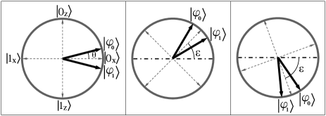
Figure 1: States of the B92 protocol with a characteristic angle $\theta=\frac{\pi}{12}$ ($15^{\circ}$). Left: channel without phase-drift, $\varepsilon=0$. Center:  channel with a phase-drift of $\varepsilon=\frac{\pi}{4}$  ($45^{\circ}$). Right: channel with a phase-drift of $\varepsilon=-\frac{7}{18}\pi$ ($-70^{\circ}$). The phase-drift rotates the reference system during the transfer of the quantum states from the transmitter to the receiver BRS07 .

Although the phase drift model can appear naive, it applies to a vast number of QKD setups, precisely to all those in which the information is encoded in the relative phase of a photon passing through an unbalanced interferometer B92 ; GRT+02 . To show how relevant it is and to facilitate a comparison between our proposal and existing solutions, we give in the next a brief overview of the main techniques used to compensate the phase drift.

One popular solution is to multiplex in the same channel the quantum signals, e.g. single-photon pulses or attenuated laser pulses, and the classical ones, e.g. intense light-pulses MT95 ; YS05 . In this way a technique already employed in classical communications is adapted to the quantum realm, but carries a few drawbacks though. First, it has been recently shown that nonlinear effects due to the propagation of intense light pulses in optical fibers can generate noise in the sensitive single-photon detectors, thus limiting in practice the maximum distance of a fiber-based QKD SZT05 . Second, the co-existence in the same channel of dim and bright pulses makes it hard to control the intensity of the incoming light, and this can be exploited by an eavesdropper to hack the QKD system Mak09 . Finally this technique requires additional hardware to be implemented.

A similar analysis holds for those systems which use a two-way configuration to enable a passive compensation of the phase-drift ZGG+97 . Indeed the pulse sent in the forward direction is necessarily intense, thus causing Rayleigh backscattering and opening the door to an interrogation attack VMH01 . Moreover, this technique cannot be employed with a single-photon source, even if some attempts have been done in this direction LM05 .

There also exist solutions which employ quantum signals only. In one case MBH04 the quantum transmission is interrupted and a sequence of quantum signals with a fixed phase value acting as a reference is sent by the transmitter along the channel until the receiver announces that the alignment has been completed . In another case EPS+03 the quantum signals with a fixed phase value are inserted in the communication using a different wavelength, like in the classical frequency-multiplexing technique. Both of these solutions have some disadvantages. In the former, the interruption of the quantum transmission represents an idle cycle from which no secure bit can be distilled; moreover this technique is not adaptive, i.e. the system cannot adapt the interruption frequency to the real noise present on the channel. In the latter, the presence of an extra wavelength implies that single-photon detectors and electronics must deal with two wavelengths rather than one, thus increasing the complexity of the setup and reducing the key generation rate due to the fewer detector’s windows available for the signal states.

Our solution represents an alternative way to control the channel noise at the quantum level without any of the above drawbacks. The necessary resources for the control are borrowed from the asymmetry of the same signals used for the very QKD process. So there is no need to multiplex quantum signal with suitably tailored bright or reference pulses, or to interrupt the quantum communication at all.

To explain in detail how the compensation technique works it is useful to recall the B92 protocol encoding-decoding mechanism B92 . Let us write explicitly the quantum states of the protocol:

$$|\varphi_{j}\rangle = \beta|0_{x}\rangle+(-1)^{j}\alpha|1_{x}\rangle,$$ (1)

$$|\overline{\varphi}_{j}\rangle = \alpha|0_{x}\rangle-(-1)^{j}\beta|1_{x}\rangle.$$ (2)

In the above equation $|\varphi_{j}\rangle$ are the signal states of the protocol and $|\overline{\varphi}_{j}\rangle$ are the states orthogonal to them, with $j=\{0,1\}$; $|0_{x}\rangle$ and $|1_{x}\rangle$ are the eigenstates of the Pauli operator X; $\beta=\sqrt{1-\alpha^{2}}=\cos(\theta/2)$ and $\theta$ belongs to the open interval $(0,\pi/2)$.

To start the communication, Alice chooses at random the value of the bit $j$, encodes it in the corresponding state $|\varphi_{j}\rangle$ and transmits it to Bob. The resulting density matrix $\rho$ prepared by Alice is then:

$$\rho = \left(|\varphi_{0}\rangle\langle\varphi_{0}|+|\varphi_{1}\rangle\langle\varphi_{1}|\right)/2$$ (3)

$$= \beta^{2}|0_{x}\rangle\langle 0_{x}|+\alpha^{2}|1_{x}\rangle\langle 1_{x}|.$$

It can be easily verified that the above density matrix is asymmetric because it is not proportional to the identity operator in the 2-dimension Hilbert space, $\textbf{I}=|0_{x}\rangle\langle 0_{x}|+|1_{x}\rangle\langle 1_{x}|$. This is a consequence of the strict nonorthogonality of the B92 protocol states. To decode the information, Bob measures the incoming states in the basis $\textbf{B}_{k}=\{|\varphi_{k}\rangle,|\overline{\varphi}_{k}\rangle\}$, $k=\{0,1\}$. Upon obtaining the state $|\overline{\varphi}_{k}\rangle$, Bob decodes Alice’s bit as $j=k\oplus 1$ (the symbol $\oplus$ means “addition modulo 2”) and labels the result as conclusive; on the contrary, upon obtaining the state $|\varphi_{k}\rangle$, Bob is not able to decode Alice’s bit deterministically, and simply labels the result as inconclusive. For example, if Bob detects the state $|\overline{\varphi}_{0}\rangle$, then he can say with certainty that the prepared state was $|\varphi_{1}\rangle$, because $|\varphi_{0}\rangle$ is orthogonal to the detected state. The same is true for the detection of $|\overline{\varphi}_{1}\rangle$, which indicates that $|\varphi_{0}\rangle$ was prepared. These are examples of conclusive results. On the contrary, if Bob detects the state $|\varphi_{0}\rangle$, he will not be able to deterministically infer Alice’s preparation, because that state has a nonzero probability to come either from $|\varphi_{0}\rangle$ or from $|\varphi_{1}\rangle$. Hence this is an example of inconclusive result.

The heart of our technique is that the asymmetric density matrix of Eq.(3) produces different amounts of conclusive and inconclusive results in Bob’s measure. In particular the ratio between inconclusive and conclusive counts is a function of the angle $\theta$, known to the users, and of the noise. Bob can estimate it during the quantum transmission thus obtaining, in real time, information about the noise, useful to eventually compensate it.

To establish the connection with the noise, let us consider a communication channel affected by the phase-drift model of noise (Fig. 1). In this case the density matrix seen by Bob is no more the one given by Eq.(3) but rather a new matrix $\widetilde{\rho}$ composed by the noise-affected quantum states $|\widetilde{\varphi}_{0}\rangle$ and $|\widetilde{\varphi}_{1}\rangle$. These states can be obtained by rotating those of Eq.(1) through the operator $\textbf{U}_{\varepsilon}=\exp\left(i\frac{\varepsilon}{2}\textbf{Y}\right)$, with Y the usual Pauli operator and $\varepsilon$ the misalignment angle:

$$\left|\widetilde{\varphi}_{0}\right\rangle = \cos[(\theta+\varepsilon)/2]\left|0_{x}\right\rangle+\sin[(\theta+\varepsilon)/2]\left|1_{x}\right\rangle,$$ (4)

$$\left|\widetilde{\varphi}_{1}\right\rangle = \cos[(\theta-\varepsilon)/2]\left|0_{x}\right\rangle-\sin[(\theta-\varepsilon)/2]\left|1_{x}\right\rangle.$$ (5)

From the density matrix $\widetilde{\rho}$ is then possible to calculate the various probabilities associated to Bob’s measurement. To make our description more realistic we introduce the quantity $\eta$, which is the probability to detect a single-photon state, i.e. a state different from a vacuum or a multi-photon state. It can be thought as a sort of total transmission of the QKD setup, including the transmission of the communication channel, $\eta_{C}$, the efficiency of Bob’s detectors, $\eta_{B}$, and the probability of double clicks in Bob’s detectors B92a . With this in mind, we write down the probability that Bob gets an inconclusive outcome, $P_{k}^{inc}=\eta\left\langle\varphi_{k}\right|\widetilde{\rho}\left|\varphi_{k}\right\rangle$, or a conclusive outcome, $P_{k}^{con}=\eta\left\langle\overline{\varphi}_{k}\right|\widetilde{\rho}\left|\overline{\varphi}_{k}\right\rangle$, when he measures in the basis $\textbf{B}_{k}$:

$$P_{k}^{inc} = \eta\{2+\cos\varepsilon+\cos[2\theta-(-1)^{k}\varepsilon]\}/4$$ (6)

$$P_{k}^{con} = \eta\{2-\cos\varepsilon-\cos[2\theta-(-1)^{k}\varepsilon]\}/4.$$ (7)

The ratio $R_{k}$ of the two above probabilities is independent of $\eta$ and is a crucial quantity, called control function:

$$R_{k}(\theta,\varepsilon)=\frac{2+\cos\varepsilon+\cos[2\theta-(-1)^{k}\varepsilon]}{2-\cos\varepsilon-\cos[2\theta-(-1)^{k}\varepsilon]}.$$ (8)

A few examples of $R_{k}$ are plotted in Fig. 2; the parameters used to draw the curves are $k=\{0,1\}$ and $\theta=\{\frac{5\pi}{18},\frac{\pi}{3},\frac{4\pi}{9}\}$. Among these curves, some are better than others to drive the noise-compensation mechanism. If the absolute value of $R_{k}$ is too small, like for the curves with $\theta=\frac{4\pi}{9}$, the system is less responsive i.e. big changes of $\varepsilon$ cause small changes of $R_{k}$. In this case the risk is that the misalignment angle becomes too large before Bob becomes aware of it and applies the correction mechanism. On the contrary, the higher the $R_{k}$ the fewer the conclusive counts registered by Bob. This results in larger fluctuations in the estimation of $R_{k}$, thus worsening the compensation mechanism, as it happens for example to the curves featuring $\theta=\frac{5\pi}{18}$ in Fig. 2. So the best option is to choose an intermediate value of $\theta$ that at the same time provides Bob with a good statistics and a responsive control. By consequence we choose $\theta=\frac{\pi}{3}$ ($60^{\circ}$) and plot in Fig. 2 the corresponding control functions together with their tangents in the zero-noise point. Such a value of $\theta$ is also interesting because it allows to merge in a single protocol the present technique and that described in LDT09 , that is an efficient long-distance version of the B92 protocol featuring an optimal $\theta$ of about $0.3\pi$ (precisely, $55.4^{\circ}$ LDT09 ).

When the noise is small, the control functions of Eq.(8) can be well approximated by their tangents in the zero-noise point; furthermore they are monotone, so only one control function, either $R_{0}$ or $R_{1}$, is sufficient to provide a reliable estimation of $\varepsilon$. This makes the feedback response very fast and we refer to this situation as to a “fast feedback”. On the contrary, when the noise is large and falls outside the monotonicity range of the control functions, Bob must use both the control functions to estimate unambiguously the misalignment angle $\varepsilon$ in the open interval $(-\pi,\pi)$. This procedure is intrinsically slower than the previous one, so we term it “slow feedback”. From a practical point of view, both the options are helpful. For example, at the beginning of a communication the users’ apparatuses are completely misaligned and $\varepsilon$ can be quite large; Bob will then use the slow feedback to get a first estimation of $\varepsilon$ and compensate it; after that, when the boxes are nearly aligned, Bob will use the fast feedback to improve the alignment and maintain it during the remaining quantum transmission.

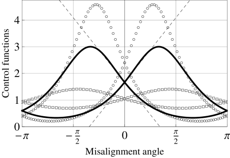
Figure 2: Examples of control functions $R_{k}(\theta,\varepsilon)$ versus the misalignment angle $\varepsilon$. The $R_{0}$ curves ($R_{1}$ curves) reach their maximum in the right-part (left-part) of the figure. The figure shows that a given misalignment angle causes a correspondent value in the control functions. Bob can exploit this correspondence to measure the control functions and from that ascertain the value of the misalignment angle.
The $R_{k}(\frac{\pi}{3},\varepsilon)$ are drawn with solid lines; the $R_{k}(\frac{5\pi}{18},\varepsilon)$ with empty circles; the $R_{k}(\frac{4\pi}{9},\varepsilon)$ with empty squares. The tangents to $R_{k}(\frac{\pi}{3},\varepsilon)$ in the zero-noise point are in dashed lines.

At this point let us mention a possible experimental implementation of the mechanism used to correct the noise. The QKD layout we are interested in is the one based on the relative-phase degree of freedom, in a one-way configuration. It is constituted by two identical interferometers placed in Alice’s and Bob’s stations B92 . Each of the interferometers features two unequal paths which provide the traveling pulses with a different amount of optical phase. The phase difference can be easily modulated by the users, who are then able to encode information in this way. In particular, the output ports of the receiver’s interferometer are usually connected with two detectors that determine the conclusiveness or inconclusiveness of a certain result.

To correct the noise, Bob executes his measurement for a while, registering all the results in a computer memory. Then, when a sufficient number of occurrences is available, Bob estimates the control functions of Eq.(8) and obtains a value of the misalignment angle $\varepsilon$. The last thing Bob has to do is to recalibrate his phase-modulator with the obtained value to re-establish the correct alignment of his apparatus with Alice’s. The read-and-write procedure just described is performed by Bob in-course-of-action, and can be easily implemented by an electronic feedback loop in which the estimated value of $R_{k}(\theta,\varepsilon)$ is the input, the fixed value of $R_{k}(\theta,0)$ is the setpoint, and a function of these two quantities is the output.

We have carried out numerical simulations of such an active feedback loop in the case of $\theta=\frac{\pi}{3}$ and the results are reported in Fig. 3.

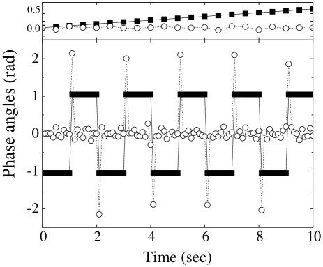
Figure 3: Noise patterns and feedback responses versus time. Top: linear noise with a rate of $0.05$ rad/sec (filled squares) and response after fast feedback is applied with a statistics of $5\times 10^{3}$ events per point (empty circles). The mean angle after feedback is $\varepsilon_{fb}^{fast}=(0.023\pm 0.031)~{}\textrm{rad}$. Bottom: step noise with amplitude 2 rad (filled squares) and response after slow feedback is applied with a statistics of $10^{3}$ events per point (empty circles). Other parameters used are (see text): $\theta=\frac{\pi}{3}$, $f=2$ MHz, $\mu=0.5$, $\eta_{B}=10\%$, $\eta_{C}=0.1$.

In the upper part of the figure we considered a linear increase in time of the misalignment angle, with a rate equal to $0.05$ rad/sec. This value is easily attainable with some care in the shielding process of the users’ interferometers against external thermal fluctuations. Phase drift values reported in the literature are well below our threshold, e.g. $0.033$ rad/sec in MBH04 or $0.0086$ rad/sec in EPS+03 . We have also assumed a trigger rate $f=2$ MHz, an average photon number per pulse $\mu=0.5$, a detector efficiency $\eta_{B}=10\%$, a channel transmittance $\eta_{C}=0.1$, equal to about $50$ km of a standard optical fiber in the third Telecom window. Multiplied together, these values provide Bob with a number of non-vacuum events per second of the order of $10^{4}$. Let us note that this represents a wide underestimation of the current QKD performances (see e.g. YDD+08 ). Each point of the plotted curves is the result of an average of $5\times 10^{3}$ acquisitions, obtained in practice by applying a feedback kick every half a second. Following the approach in EPS+03 , we have empirically verified the optimality of this value: if larger, the phase-drift would become too big in the between of two consecutive feedback kicks; if smaller, the statistical error pertaining to Bob’s measurement would increase considerably. The empty circles in the upper part of Fig. 3 show the response of the fast feedback loop, i.e. the one in which a linear approximation of the control functions is adopted. In particular we used the first-order expansion of $R_{0}(\frac{\pi}{3},\varepsilon)$ in $\varepsilon=0$ to drive the feedback. With feedback, the mean misalignment angle of the communication channel reduces to:

$$\varepsilon_{fb}^{fast}=(0.023\pm 0.031)~{}\textrm{rad}.$$ (9)

The slight bias towards positive values is due to the monotone increase of the phase-drift. The standard deviation is well below the amount of phase-drift accumulated every second on the channel.

In the lower part of Fig. 3 we have considered a phase-drift in the form of a step-function of amplitude equal to $2$ rad, to study the response of the slow feedback loop in the case of a large phase-drift. In this case Bob exploits both $R_{0}(\frac{\pi}{3},\varepsilon)$ and $R_{1}(\frac{\pi}{3},\varepsilon)$ to estimate the misalignment angle. After acquiring $10^{3}$ events he evaluates the mean values of $R_{0}$ and $R_{1}$, let us term them $R_{0}^{*}$ and $R_{1}^{*}$. Then he numerically finds the point $\varepsilon^{*}$ that minimizes the quantity $|R_{0}(\frac{\pi}{3},\varepsilon)-R_{0}^{*}|$ $+$ $|R_{1}(\frac{\pi}{3},\varepsilon)-R_{1}^{*}|$. He finally uses the value of $\varepsilon^{*}$ to compensate the phase-drift. The empty circles of the figure again represent the value of the misalignment angle after the feedback has been applied. It can be seen that in correspondence of the noise steps the angle seen by Bob undergoes strong jumps, but the system recovers immediately after the jump. If one ignores the jumps, the mean misalignment angle is:

$$\varepsilon_{fb}^{slow}=(-0.002\pm 0.098)~{}\textrm{rad}.$$ (10)

Compared to Eq.(9), the average value is nearly unbiased, following the unbiased behavior of the noise, while the standard deviation is more than three times bigger due to the reduced statistics adopted for this kind of feedback. It can be nice to note that the step-noise pattern of Fig.3 could be employed by the users to create an additional communication channel between them. More explicitly, Alice could purposely feed into her phase-modulator a large phase value in order to send some sort of message to Bob, like e.g. a string of bits useful to identify a certain part of the quantum transmission.

As a last point of our work we want to establish whether the results of Eqs. (9) and (10) are good enough for a practical implementation of the B92 protocol. In particular we calculate the maximum misalignment angle for which the secure gain of the B92 protocol is still positive. The secure gain of a protocol is the ratio between the number of secure bits distilled and the number of qubits prepared by Alice. For the B92 protocol it is defined as $G=\Lambda_{con}[1-h(\frac{\Lambda_{bit}}{\Lambda_{con}})-h(\frac{\overline{\Lambda}_{ph}}{\Lambda_{con}})]$, with $h$ the Shannon entropy, $\Lambda_{con}$ the conclusive-count rate, $\Lambda_{bit}$ the bit-error rate and $\overline{\Lambda}_{ph}$ the upper bound to the phase-error rate obtained from $\Lambda_{bit}$ and $\Lambda_{con}$ through an optimization algorithm B92a ; LDT09 .

The bit-error rate is given by the probability that Bob finds the state $\left|\overline{\varphi}_{0}\right\rangle$ ($\left|\overline{\varphi}_{1}\right\rangle$) when Alice prepares the orthogonal state $\left|\varphi_{0}\right\rangle$ ($\left|\varphi_{1}\right\rangle$). For the present discussion it suffices to assume that the phase-drift is the only source of errors; in reality there are also the detector dark counts and the unavoidable experimental imperfections. By using the noisy states of Eqs. (4) and (5), and assuming a preparation of the bit value 0 (the same holds for the bit value 1), we obtain the following bit-error rate:

$$\Lambda_{bit} = \eta(\left|\left\langle\widetilde{\varphi}_{0}|\overline{\varphi}_{0}\right\rangle\right|^{2})/2$$ (11)

$$= \eta\left(1-\cos\varepsilon\right)/4.$$

This expression is independent of $\theta$ and correctly vanishes when $\varepsilon$ tends to zero. The coefficient $\eta$ takes into account the vacuum or multi-photon counts by Bob, while the factor $1/2$ is the probability to guess the right basis to detect the error.

In a similar way, the conclusive-count rate is given by the probability that Bob obtains a conclusive result, and can be evaluated from the mean value of $P_{0}^{con}$ and $P_{1}^{con}$ in Eq. (7):

$$\Lambda_{con} = (P_{0}^{con}+P_{1}^{inc})/2$$ (12)

$$= \eta(1-\cos\varepsilon\cos^{2}\theta)/2.$$

This time, there is a dependance on $\theta$. After fixing $\theta=\frac{\pi}{3}$ and using Eqs. (11) and (12), we have numerically found a positive gain for the B92 protocol until

$$|\varepsilon|<0.27646~{}\textrm{rad}.$$ (13)

The value of $\varepsilon$ given by the fast feedback, Eq. (9), is much smaller than the above threshold. Hence our proposal appears feasible, especially if one considers that we made conservative assumptions on the QKD parameters and that less conservative assumptions would lead to better values in Eqs. (9) and (10).

Let us point out that Eqs. (11) and (12) establish a direct dependance of the bit-error rate and conclusive-count rate on the misalignment angle $\varepsilon$. This allows Bob to estimate $\Lambda_{bit}$ and $\Lambda_{con}$ without communicating with Alice. It suffices that Bob gets an estimate of $\varepsilon$ from his data and substitutes it into the given equations note2 . This is a further peculiarity of the B92 protocol that remained unnoticed so far. It can considerably increase the practicality of the protocol by reducing the classical communication necessary to distill the final key.

In conclusion, we introduced a novel scheme to detect and correct the phase-drift of a communication channel based on some characteristics of the B92 protocol not considered so far. The scheme features a few remarkable properties: it is entirely quantum, it can be executed real-time without interrupting the communication, it allows to estimate the bit-error rate without a bidirectional communication, it creates additional communication channels for the users. This highly increases the practicality of the B92 protocol, often considered unsuitable for real-world implementations. Furthermore, the fully quantum nature of the scheme on one side reduces the noise due to the propagation of high-intensity light pulses in a nonlinear medium, on the other makes it conceivable the construction of networks and devices working entirely at the quantum level, thus preventing several hacking strategies available to Eve. The asymmetry-based correction mechanism can be extended to the polarization degree of freedom and can play a role in the entanglement distribution problem.

References

- (1) N. Gisin, G. Ribordy, W. Tittel and H. Zbinden, Rev. Mod. Phys. 74, 145 (2002).
- (2) C. H. Bennett, Phys. Rev. Lett. 68, 3121 (1992).
- (3) K. Tamaki, M. Koashi, and N. Imoto, Phys. Rev. Lett. 90, 167904 (2003); K. Tamaki and N. Lütkenhaus, Phys. Rev. A 69, 032316 (2004).
- (4) M. Koashi, Phys. Rev. Lett. 93, 120501 (2004); K. Tamaki, N. Lütkenhaus, M. Koashi, and J. Batuwantudawe, Phys. Rev. A 80, 032302 (2009); K. Tamaki, ibid. 77, 032341 (2008).
- (5) M. Lucamarini, G. Di Giuseppe, and K. Tamaki, Phys. Rev. A 80, 032327 (2009).
- (6) M. Born and E. Wolf, Principles of Optics, 7th (expanded) edition, Cambridge University Press (1999).
- (7) S. D. Bartlett, T. Rudolph, and R. W. Spekkens, Rev. Mod. Phys. 79, 555 (2007).
- (8) C. Marand and P. Townsend, Opt. Lett. 20, 1695 (1995).
- (9) Z. L. Yuan and A. J. Shields, Opt. Expr. 13, 660 (2005).
- (10) D. Subacius and A. Zavriyev and A. Trifonov, Appl. Phys. Lett. 86, 011103 (2005).
- (11) V. Makarov, New J. Phys. 11, 065003 (2009).
- (12) H. Zbinden, J. D. Gautier, N. Gisin, B. Huttner, A. Muller, and W. Tittel, Electron. Lett. 33, 586 (1997).
- (13) A. Vakhitov, V. Makarov, and D. R. Hjelme, J. Mod. Opt. 48, 2023 (2001).
- (14) M. Lucamarini and S. Mancini, Phys. Rev. Lett. 94, 140501 (2005); A. Cerè, M. Lucamarini, G. Di Giuseppe, and P. Tombesi, ibid. 96, 200501 (2006); R. Kumar, M. Lucamarini, G. Di Giuseppe, R. Natali, G. Mancini, and P. Tombesi, Phys. Rev. A 77, 022304 (2008).
- (15) V. Makarov, A. Brylevski, and D. R. Hjelme, Appl. Opt. 43, 4385 (2004).
- (16) B. B. Elliott, O. Pikalo, J. Schlafer, and G. Troxel, Proc. SPIE 5105, 26 (2003).
- (17) Z. L. Yuan, A. R. Dixon, J. F. Dynes, A. W. Sharpe, and A. J. Shields, Appl. Phys. Lett. 92, 201104 (2008).
- (18) Since Bob knows the expected number of single-photon events, he can easily appraise from the single-photon events effectively registered by his measuring device.