Phase separation and pairing regimes in the one-dimensional asymmetric Hubbard model

Abstract

We address some open questions regarding the phase diagram of the one-dimensional Hubbard model with asymmetric hopping coefficients and balanced species. In the attractive regime we present a numerical study of the passage from on-site pairing dominant correlations at small asymmetries to charge-density waves in the region with markedly different hopping coefficients. In the repulsive regime we exploit two analytical treatments in the strong- and weak-coupling regimes in order to locate the onset of phase separation at small and large asymmetries respectively.

I Introduction

In this paper we study a variation of the one-dimensional Hubbard model (HM) in which the difference between the hopping amplitudes, say $t_{\uparrow}>t_{\downarrow}$, is responsible for an explicit breaking of the rotational symmetry. It is described by the Hamiltonian

$$H=-\sum_{j\sigma}t_{\sigma}(c_{j\sigma}^{\dagger}c_{j+1\sigma}+{\rm h.c.})+U\sum_{j}n_{j\uparrow}n_{j\downarrow}$$ (1)

where $c_{j\sigma}$ denotes the annihilation operator of a fermion with $\sigma=\uparrow,\downarrow$ at site $j$ and $n_{j\sigma}=c_{j\sigma}^{\dagger}c_{j\sigma}$ are the associated number operators.

This asymmetric Hubbard model (AHM) has been studied in the past FK1969 to describe the essential features of the metal-insulator transition in rare-earth materials and transition-metal oxides; in this case $\sigma$ represents two types of spinless fermions (the real spin being considered not essential for the transition to be modelled). The “light” particles are described by band (Bloch) states, while the “heavy” ones tend to be localized on lattice (Wannier) sites. More recently, this model has gained a renewed interest in experiments with optical lattices, in which both the effective strengths of the kinetic and of the potential parts can be varied in a rather controlled way, including the possibility of reaching the attractive regime $U<0$. The possibility to use cold atoms BDZ2008 ; Jetal1998 to engineer condensed matter systems with a high tunability offers an experimental way to test theoretical results with great accuracy. Two-species models with different hopping coefficients can also be realized by trapping atomic clouds with two internal states of different angular momentum, thereby introducing a spin dependent optical lattice, which enables to modify the ratio $a=t_{\downarrow}/t_{\uparrow}$ by controlling the depth of the optical lattice LWZ2004 . Yet another possibility is to trap two different species of fermionic atoms, so that the “anisotropy” $a$ is given naturally by the ratio of masses. In the context of cold atoms in optical lattices the subscripts $\sigma=\uparrow,\downarrow$ are not related to the electron spin but label the two different species of fermions, either different atoms with half-integer spin or different excited states of one atomic specie with fine structure splitting.

Many recent papers on the subject are devoted to the onset of the so-called Fulde-Ferrell-Larkin-Ovchinnikov (FFLO) phase, which may occur with unbalanced species BWHR2009 ; WCDS2009 . In this paper we will consider instead the case of balanced species: $N_{\uparrow}=N_{\downarrow}$. The parameters that influence the phase diagram can be cast in the form of an anisotropy coefficient $z=(t_{\uparrow}-t_{\downarrow})/(t_{\uparrow}+t_{\downarrow})=(1-a)/(1+a)$ and a dimensionless onsite potential $u=U/t$, where $t=(t_{\uparrow}+t_{\downarrow})/2$ is an overall energy scale. In addition one can consider the effect of the total filling $n=N/L$, $N$ being the total number of fermions and $L$ the chain length. At variance with the typical situation in condensed matter physics, where the bulk filling and magnetization $m^{z}=(n_{\uparrow}-n_{\downarrow})/2$ are controlled in a grand-canonical framework by the chemical potential and an external magnetic field respectively, in the context of cold atoms it is conceivable to fix independently the number of particles in each of the two species, despite the fact that only a given choice of the densities $n_{\uparrow}$ and $n_{\downarrow}$ might correspond to the absolute minimum of the grand potential. Henceforth we will assume that they are equally populated, that is $n_{\uparrow}=n_{\downarrow}=n/2$ and we will limit ourselves to $n<1$. Note that if $E(n,m^{z})$ is the energy in a given sector of $n$ and $m^{z}$ (these two quantities are good quantum numbers also in the asymmetric case), then a particle-hole transformation $n_{j\sigma}\to(1-n_{j\sigma})$ leads to $E(2-n,-m^{z})=E(n,m^{z})-UL(n-1)$, so that for $m^{z}=0$ it is sufficient to analyze the phase diagram for positive and negative $U$ and $n<1$, in order to infer features also at $n>1$. The phase diagram at half-filling, $n=1$, has been studied in ref. FDL1995 , soon after the development of White’s density-matrix renormalization group (DMRG) method W1993 . The limiting case of the symmetric HM $(z=0)$ can be solved exactly via the Bethe ansatz approach LW1968 . The opposite extremal case $z=1$ is usually called the Falicov-Kimball (FK) model. In any dimensionality, it has been proved FLU2002 that for large positive $U$ and $n\neq$1 the system has a ground state characterized by a spatially non-homogeneous density profile where the heavy particles are compressed in a region with length $L_{\downarrow}=N_{\downarrow}$. In this paper we refer to this phase as totally segregated state (TSS). A similar phase, where the heavy particles acquire a finite kinetic energy ($L_{\downarrow}>N_{\downarrow}$), appears for $z\lesssim 1$ U2004 and can be interpreted as the result of an effective attractive interaction between light fermions, mediated by the heavy ones (see DLE1995 in 1D and DLF1996 in 2D). The latter situation is denoted in the following as phase separation (PS). A cartoon representation of the different phases is presented in Fig. 1. At smaller asymmetries, the system is instead in a more conventional spatially homogeneous phase (HP). The ground state phase diagram for the model in the $m^{z}=0$ sector has been discussed in CHG2005 by means of the bosonization approach. In this context WCG2007 the HP-PS transition line at $u>0$ has been interpreted as the curve in $(z,u)$-plane where the velocity of one of the two decoupled bosonic modes vanishes.

Let us summarize the content of this paper. In Sec. II we will study numerically the attractive regime ($U<0$), by using a DMRG program. In particular we will examine which kind of correlations (charge or pairing) is dominant in this region of the phase diagram. Then we will move to consider the repulsive ($U>0$) regime. In Sec. III we will analytically discuss the weak coupling regime ($|U|\ll t_{\sigma}$) by means of a variational method that compares the energy of the PS state with that of the HP state, the latter being calculated within a second order perturbation analysis. In Sec. IV we move to study the strong coupling regime ($U\gg t_{\sigma}$) in order to determine a phase diagram which includes also different types of PS states. The results are summarized and the conclusions are drawn in Sec. V.

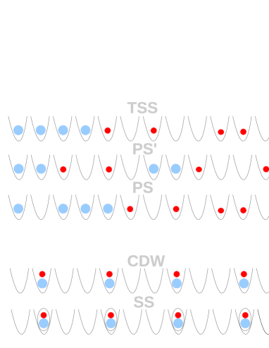
Figure 1: Schematic representation of the phases discussed in the text. Large and small disks represent heavy and light fermions respectively. The ellipsis encircling the pairs in the SS phase denote onsite pairing. The HP state defined in Eq. (2) has not been drawn in real space because it is defined directly in momentum space by filling the two noninteracting bands up to $k_{F}$.

II Singlet-pairing to charge-density wave transition at $U<0$

One of the open points raised in ref. CHG2005 is the existence of regions at $U<0$ characterized by dominating charge-density wave (CDW) correlations instead of the singlet-superconducting (SS) ones that one has in the attractive symmetric HM. On a lattice the CDW and the SS correlation functions are defined respectively as

$$C(r)=\langle n_{j}n_{j+r}\rangle-\langle n_{j}\rangle\langle n_{j+r}\rangle$$

$$P(r)=\langle\eta_{j}^{\dagger}\eta_{j+r}\rangle$$

where $n_{j}=n_{j\uparrow}+n_{j\downarrow}$ while $\eta_{j}=c_{j\downarrow}c_{j\uparrow}$ is the operator that destroys an onsite pair with singlet spin wavefunction. At large distances $r$, bosonization procedures predict Gia2003

$$C(r)\sim\frac{-K_{\rho}}{\pi^{2}r^{2}}+A\frac{\cos(2k_{F}r)}{r^{K_{\rho}+K_{\sigma}}}$$

$$P(r)\sim\frac{B}{r^{1/K_{\rho}+K_{\sigma}}}$$

where $A$ and $B$ are constants, and $K_{\rho}$ and $K_{\sigma}$ are the Luttinger parameters for the charge and spin degrees of freedom respectively. Clearly $C(r)$ dominates over $P(r)$ when $K_{\rho}<1$, while $K_{\sigma}$ has to be fixed to 0 for gapped spin phases. A numerical estimate of $K_{\rho}$ from finite-size data can be obtained as in ref. SBC2004 by considering the structure factor

$$S(q)=\sum_{r}{\rm e}^{{\rm i}qr}\langle n_{j}n_{j+r}\rangle$$

Here we have dropped the dependence on $j$ because we implicitly assume that the correlation functions are translationally invariant due to periodic boundary conditions (PBC). The value $S(q=0)$ corresponds to the average correlation and it diverges in the thermodynamic limit, since typically $\langle n_{j}n_{j+r}\rangle$ saturates at a finite value $n^{2}$ for large distances. So one may consider the connected charge correlation $C(r)$ in order to avoid this divergence. This choice affects the structure factor only at $q=0$ and bosonization predicts that the value of $K_{\rho}$ is directly related to the limit $q\to 0$

$$S(q)\simeq K_{\rho}\frac{q}{\pi}+\dots$$

Following the procedure of ref. SBC2004 by selecting the smallest possible non-vanishing momentum compatible with PBC $q_{1}=2\pi/L$ one builds a sequence that approximates the linear slope

$$K_{\rho}(L)=S(q_{1})\frac{L}{2}.$$

The dependence on $L$ indicates that the sequence has to be extrapolated to $L\to\infty$ in order to obtain the limit $q\to 0$ and the parameter $K_{\rho}$. The DMRG results corresponding to various fillings $n=0.4,\;0.6,\;0.8$ with $z=0.2,\;0.5,\;0.65,\;0.8$ and $u=-0.001,\;-0.5,\;-3$ are reported in table 1; in the caption we have reported also the relevant features of our DMRG numerical calculations. For a fixed value of $u<0$ we always find that the extrapolated $K_{\rho}$ decreases with increasing $z$. From this grid of points we can have an idea of the SS-CDW transition curve by locating the points at which $K_{\rho}=1$. This has been done interpolating the data with splines. An example of this procedure is given in Fig. 2, while the global results are plotted in Fig. 3.

In ref. CHG2005 (Fig. 1 therein) the authors report a triangular region obtained by means of bosonization at $u<0$ where the dominant correlations are CDW or SS depending on the filling. Here we observe that the shape of the transition line is indeed dependent on $n$: for $u<-0.5$ the separation line might have both a negative and a positive slope, depending on the value of $n$. For small (negative) $u$ the curve has always a negative slope. Because of the uncertainty related to DMRG and finite-size effects, our estimate of the transition points is limited to $u\leq-10^{-3}$; moving closer to $u=0$ would produce values of $K_{\rho}$ essentially always equal to 1 within the numerical error, for all values of $z$, so we have not pushed our analysis and conclusions closer to $u=0$.

Finally we should mention that a direct inspection of the charge correlation functions in real and in Fourier space reveals that the only characteristic wavenumber is $2k_{F}=\pi n$, where typically the structure factor displays a peak for $u<0$, but there is neither FFLO behavior - as expected since we have selected balanced species - nor a collapse (predicted at sufficiently large negative $u$ M2007 ).

$u$ \ $z$		$0.2$	$0.5$	$0.65$	$0.8$
	$n=0.4$
$-10^{-3}$		$1.001\pm 0.002^{\ddagger}$	$0.9978\pm 0.0002^{*}$	$0.994\pm 0.001^{*}$	$0.986\pm 0.004^{*}$
$-0.5$		$1.0700\pm 0.0004$	$1.038\pm 0.001$	$0.992\pm 0.002$	$0.906\pm 0.003$
$-3$		$1.4209\pm 0.0005$	$1.2528\pm 0.0003$	$1.0976\pm 0.0002$	$0.86715\pm 0.00005$
	$n=0.6$
$-10^{-3}$		$1.0034\pm 0.0008^{*}$	$1.001\pm 0.001^{\ddagger}$	$1.000\pm 0.002^{\ddagger}$	$0.998\pm 0.004^{\ddagger}$
$-0.5$		$1.050\pm 0.001^{\ddagger}$	$1.04\pm 0.01^{\ddagger}$	$1.03\pm 0.02^{\ddagger}$	$1.00\pm 0.05^{\ddagger}$
$-3$		$1.26016\pm 0.00007$	$1.110\pm 0.003$	$0.969\pm 0.004$	$0.751\pm 0.004$
	$n=0.8$
$-10^{-3}$		$1.008\pm 0.002^{*}$	$0.9976\pm 0.0001^{*}$	$0.983\pm 0.005$	$0.951\pm 0.009$
$-0.5$		$1.045\pm 0.005^{\ddagger}$	$1.014\pm 0.001$	$0.980\pm 0.002$	$0.913\pm 0.002$
$-3$		$1.1603\pm 0.0001$	$1.0163\pm 0.0008$	$0.880\pm 0.001$	$0.6722\pm 0.0008$

Table 1: Extrapolations for the parameter $K_{\rho}$ from DMRG simulations with PBC, $L=10,20,30,40,50$, 1100-1300 optimized states and seven finite-system sweeps. This conservative choice guarantees an energy relative error of $O(10^{-6})$ up to $L=30$ and $O(10^{-5})$ up to $L=50$ (recall that the charge degrees of freedom are always gapless). Unless otherwise specified the extrapolations have been performed using quadratic fits in $1/L$ and the error bars are evaluated according to NR (Chapter 15) using the sum of squared differences normalized to the fit degrees of freedom as a measure of the spread in the ordinates. $\ddagger$: Oscillating about reported value with spread. *: Linear fit in $1/L$.

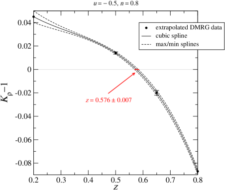
Figure 2: Example of cubic splines interpolation to locate the transition point and the associated error, using the DMRG data of table 1. The horizontal solid segment at $K_{\rho}=1$ indicates the reported interval.

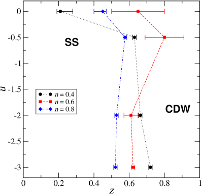
Figure 3: Numerical estimates of the transition lines from SS (on the left) to CDW (on the right) dominant correlations in the attractive regime for the values of filling reported in the legend. Not all the data used to obtain the figure have been reported in table 1. The error bars associated to the transition points have been determined by means of splines passing through the upper and lower edges of each interval of possible values of $K_{\rho}$ reported in the table (see the construction of Fig. 2); when the uncertainty in $z$ turned to be smaller than $10^{-2}$ we have conventionally set it to this value to account for the approximation introduced by cubic splines interpolation. The lines joining the points are guides for the eye.

III Weak-coupling limit

From a quantitative point of view, bosonization cannot be conclusive about the location of the HP to PS transition at $z\cong 1$. This is due to the fact that, while a continuum limit approach is justified close to $z=0$, in the FK limit even a small $U$ can involve processes away from the Fermi surface, and so the requirement $|U|\ll\min[t_{\uparrow},t_{\downarrow}]$ strictly reduces the range of reliability of this approachCHG2005 .

Numerical data F2007 indicate that in the highly asymmetric regime phase separation appears above a critical value of $U$ which approaches zero in the low-density limit.

When approaching the FK limit $z\rightarrow 1$, the kinetic energy of the lighter species becomes the dominant term of the Hamiltonian at weak coupling, $U\ll t_{\uparrow}$. For $U>0$, the competition between the light particle kinetic energy and the repulsive on-site interaction can drive the system into an instability with respect to phase separation U2004 : there exists a critical value $u_{PS}(z,n)$ above which light particles will occupy a large region of the system where $n_{i\downarrow}=0$, creating an effective pressure which confines heavy particles into a small region with density close to 1; this effect is reminiscent of the segregated regime present in the FK model in the repulsive regime.

Different numerical and analytical methods have been proposed in literature to identify this phase transition between the HP and the PS/TSS regimes WCG2007 ; Cetal2008 ; F2007 . In the following, we will (i) apply a second order perturbation theory approach, first introduced MV1989 to study the ground state of the weakly interacting symmetric HM, to compute the energy of a homogeneous phase ground state of the AHM and (ii) compare HP and PS or TSS energies in order to detect the line of quantum phase transition as a function of the original model parameters $z,u,n$. Finally, a comparison with previous results will be presented.

III.1 Trial wave functions

In the low coupling regime, we can consider as extended ground state the exact one at $U=0$ (and $t_{\downarrow}\neq 0)$, which can be obtained by filling both Fermi bands up to $k_{F\sigma}$:

$$|\Psi\rangle_{HP}=\prod_{|q|\leq k_{F\downarrow}}\tilde{c}_{q\downarrow}^{\dagger}\prod_{|k|\leq k_{F\uparrow}}\tilde{c}_{k\uparrow}^{\dagger}|0\rangle$$ (2)

where $|0\rangle$ represents the zero-fermions vacuum and $\tilde{c}_{k\sigma}^{\dagger}$ are the creation fermionic operators in Fourier space. While $|\psi\rangle_{HP}$ is not an exact eigenstate of the full Hamiltonian, perturbation theory above this ansatz have provided excellent results for $z=0$ MV1989 , where a comparison with the exact solution is possible, and, as shown later in the section, even in the highly asymmetric regime.

The PS ground state instead can be obtained in the following way: first, we confine all heavy particles in a given part of the lattice of relative length $\nu$, with $(L-N_{\uparrow})/L\geq\nu\geq N_{\downarrow}/L$; then we consider two different chains of length $L_{\downarrow}=\nu L,\;L_{\uparrow}=L(1-\nu)$ respectively and then fill the new Fermi bands till the momenta $k_{F\sigma}^{\prime}=\pi N_{\sigma}/L_{\sigma}$:

$$|\Psi(\nu)\rangle_{PS}=\prod_{|q^{\prime}|\leq k_{F\downarrow}^{\prime}}\tilde{c}_{q^{\prime}\downarrow}^{\dagger}\prod_{|k^{\prime}|\leq k_{F\uparrow}^{\prime}}\tilde{c}_{k^{\prime}\uparrow}^{\dagger}|0\rangle.$$

In practice we have to consider that the effective light-particle and heavy-particle “chain lengths” are not $L$ but $L(1-\nu)$ and $L\nu$, respectively.

In addition, we can define a TSS as the one with a completely full region of heavy particles, i.e. $\nu=N_{\downarrow}/L$. In this case, the variational wave function can be written as:

$$|\Psi\rangle_{TSS}=\prod_{(1-n_{\downarrow})L<j<L}c_{j\downarrow}^{\dagger}\prod_{|k^{\prime}|\leq k_{F\uparrow}^{\prime}}\tilde{c}_{k^{\prime}\uparrow}^{\dagger}|0\rangle.$$

where now the down-fermion creation operators are taken in real space representation. Both TSS and PS state trial wave functions are eigenstate of the Hamiltonian up to a boundary term which we neglect in the following $L\rightarrow\infty$ limit.

III.2 Ground state energies

The instability of a homogeneous ground state towards a phase separated one can be analyzed by computing the corresponding zero temperature energy:

$$\mathcal{E}_{PS}=\frac{{}_{PS}\langle\Psi|H|\Psi\rangle_{PS}}{L},\quad\mathcal{E}_{HP}=\frac{{}_{HP}\langle\Psi|H|\Psi\rangle_{HP}}{L}$$

and by comparing them to get the phase transition hypersurface in parameter space described by:

$$\mathcal{E}_{PS}(n_{\uparrow},n_{\downarrow},U,z)-\mathcal{E}_{HP}(n_{\uparrow},n_{\downarrow},U,z)=0$$

A similar criterion can be applied to distinguish between TSS and PS state without segregation, as described later in the section. We remark that in the PS region, due to the fact that within the two subchains of length $L_{\uparrow,\downarrow}$ the up and down particles do not overlap, the interaction term provides at most a boundary contribution which can be neglected in the thermodynamic limit. We will come back to this point later.

We can then compute the PS state energy density $\mathcal{E}_{PS}$ considering only the kinetic term contribution. For a general $\nu$, the result is

$$\mathcal{E}_{PS}(\nu)=-t(1+z)\frac{2(1-\nu)}{\pi}\sin\left(\frac{\pi n_{\uparrow}}{1-\nu}\right)$$ (3)

$$-t(1-z)\frac{2\nu}{\pi}\sin\left(\frac{\pi n_{\downarrow}}{\nu}\right)$$

As already stated in U2004 (in particular Sec. 3 therein), it is possible to fix the lowest energy state with respect to $\nu$ searching for a minimum of (3) at fixed densities and hopping rates. The corresponding condition $\partial_{\nu}\mathcal{E}_{PS}=0$ becomes

$$(1+z)\sin\left(\frac{\pi n_{\uparrow}}{1-\nu}\right)-\frac{\pi n_{\uparrow}}{1-\nu}\cos\left(\frac{\pi n_{\uparrow}}{1-\nu}\right)$$

$$=(1-z)\left[\sin\left(\frac{\pi n_{\downarrow}}{\nu}\right)-\frac{\pi n_{\downarrow}}{\nu}\cos\left(\frac{\pi n_{\downarrow}}{\nu}\right)\right]$$ (4)

If there exists a value of $\nu$, $\nu^{*}$ with $1-n_{\uparrow}>\nu^{*}>n_{\downarrow}$, which satisfies this condition, then the lowest energy state is $|\Psi(\nu^{*})\rangle_{PS}$; otherwise, the minimum of $\mathcal{E}_{PS}$ lies on the boundary $\nu^{*}=n_{\downarrow}$ and TSS is energetically more favorable. The boundary between these two regions is described by the condition $\partial{\cal E}_{PS}/\partial\nu|_{\nu=n_{\downarrow}}=0$; the solution of this equation provides a characteristic anisotropy coefficient $\bar{z}$ for given $n_{\uparrow,\downarrow}$ that turns out to be independent of $u$. We expect that $\bar{z}$ represents a good estimate for the phase transition between TSS and $\nu\neq n_{\downarrow}$ states even at intermediate couplings. In fact, we find good agreement with the values corresponding to the (almost) horizontal lines plotted in Fig. 3 of ref. F2007 .

As said before, here we consider only the balanced case $n_{\uparrow}=n_{\downarrow}=n/2$, for which the condition that yields the optimal $\nu=\nu^{*}(z)$ in the range $\nu\in(n/2,1-n/2)$ simplifies to

$$z=\frac{f\left(\frac{\pi n}{2\nu}\right)-f\left(\frac{\pi n}{2(1-\nu)}\right)}{f\left(\frac{\pi n}{2\nu}\right)+f\left(\frac{\pi n}{2(1-\nu)}\right)}$$ (5)

with $f(x)=\sin x-x\cos x$. The upper limit for $\nu$ is formally obtained by compressing the up-fermions so that $1-\nu=n/2$. When $\nu=1/2$ the numerator of the right-hand side vanishes and $z$ reaches the minimum possible value $z=0$. When $\nu=\nu_{min}=n/2$ the right-hand side has the value

$$\bar{z}(n)=\frac{\pi-f(\pi n/(2-n))}{\pi+f(\pi n/(2-n))}.$$

This function decreases monotonically with the filling from $\bar{z}(0)=1$ to $\bar{z}(1)=0$. If $z\geq\bar{z}(n)$, the minimum energy is attained at the lower limit $\nu^{*}=n/2$, corresponding to maximum compression of the down-fermions, independently of the value of $z$. Clearly, high densities favor a TSS state, since a large amount of light particles produce a sufficient pressure in order to compress all heavy particles in a very small region. When the density is low enough, this condition cannot be satisfied, except at very large mass imbalances, and heavy particles still contribute to the kinetic energy of the system. Fig. 4 shows an example of such a construction for $n=1/2$.

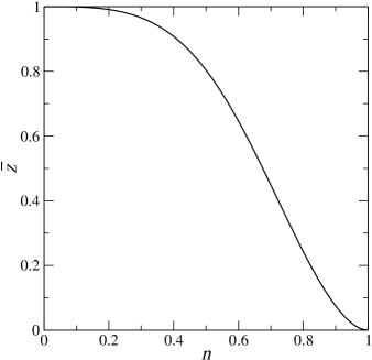
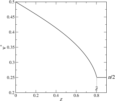
Figure 4: Upper panel: Plot of the function $\bar{z}(n)$. Lower panel: Optimal value of $\nu$ as a function of $z$ in the whole interval $[0,1]$ for filling $n=1/2$.

The energy density of the HP state receives instead both kinetic and interaction contributions: $\mathcal{E}_{HP}=\mathcal{E}_{T}+\mathcal{E}_{U}$. The kinetic part is equivalent to the ground state energy density of the non-interacting case

$$\mathcal{E}_{T}=-t(1+z)\frac{2}{\pi}\sin(\pi n_{\uparrow})-t(1-z)\frac{2}{\pi}\sin(\pi n_{\downarrow})$$ (6)

whereas the interacting part in the weak coupling limit can be expressed as a series in $U$ applying a second order perturbation theory MV1989 :

$$\mathcal{E}_{U}=\frac{1}{L}\,_{HP}\langle\Psi|H_{U}|\Psi\rangle_{HP}$$

$$+\frac{1}{L}\left({}_{HP}\langle\Psi|H_{U}\frac{1}{\mathcal{E}_{T}-H_{0}}H_{U}|\Psi\rangle_{HP}\right)_{{\rm conn}}+\mathcal{O}(U^{3})$$

where $(...)_{{\rm conn}}$ indicates a sum over connected diagrams and $H_{0}$ denotes the unperturbed Hamiltonian. The first order contribution is obtained rewriting the number operators in momentum space, thus obtaining

$${}_{HP}\langle\Psi|H_{U}|\Psi\rangle_{HP}=LUn_{\uparrow}n_{\downarrow}$$ (7)

while the second order contribution can be computed evaluating Goldstone diagrams:

$$\mathcal{E}_{HP}^{(2)}=-\frac{U^{2}}{t(2\pi)^{3}}\frac{\vartheta(k_{F\uparrow},k_{\downarrow},a)}{(1+z)}$$ (8)

$$\vartheta(k_{F\uparrow},k_{\downarrow},a)\equiv\int_{0}^{\frac{\pi}{2}}\frac{dq}{\sin q}\int_{-q}^{q}\;dk\times$$

$$\times\int_{-q}^{q}\frac{dk^{\prime}}{\sin(k+k_{F\uparrow})+a\sin(k^{\prime}+k_{F\downarrow})}.$$

Integrating the previous expression numerically, we can give a quantitative estimate of the phase boundary near the FK limit. Furthermore, by comparing ${\cal E}_{HP}$ up to second order (plotted in Fig. 5) with previous numerical results F2007 , we have a good check that at half filling the variational ground state (2) is a correct description of the system even at finite $U/t_{\uparrow}\leq 3$.

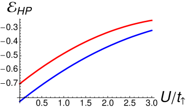
Figure 5: Energy density of the HP state at $n=1$ for different asymmetry parameters: upper red line $t_{\downarrow}/t_{\uparrow}=0.1$, lower blue line $t_{\downarrow}/t_{\uparrow}=0.3$.

III.3 Phase boundaries

The weak-coupling phase diagram is generally characterized by two types of phase transition: one between the HP state and the PS region, and the other one between different types of spatially separated states.

Combining Eqs.(3), (6), (7) and (8), the first mentioned phase transition line is determined by the equation:

$$2\sin\left(\frac{\pi n}{2}\right)-(1+z)\frac{2-n}{2}\sin\left(\frac{\pi n}{2-n}\right)=$$

$$\frac{\pi}{2}u\left[\frac{n^{2}}{4}-u\frac{\vartheta(k_{F\uparrow},k_{F\uparrow},a)}{(2\pi)^{3}(1+z)}\right]$$ (9)

Table 2 shows how the correlated energy factor depends on $k_{F\uparrow}$ and $z=(1-a)/(1+a)$. In general, the larger the asymmetry $z$ is (the smaller is $a)$ the larger is $\vartheta$. An illustrative plot at half-filling is presented in Fig. 6. Furthermore $\vartheta$ approaches 0 in the low-density limit and grows with the filling.

$a\backslash k_{F\downarrow}=\pi n/2$	$\pi/3$	$\pi/4$	$\pi/6$
0.01	0.028	0.022	0.013
0.05	0.027	0.021	0.012
0.1	0.026	0.02	0.012
0.15	0.025	0.019	0.012
0.2	0.024	0.018	0.011

Table 2: Numerical values for $\vartheta(k_{F\uparrow},k_{F\uparrow},a)/(2\pi)^{3}$ below half filling. Notice that the term $(1+z)$ in the denominator of Eq. (8) has not been included in the definition of $\vartheta$ so to have a more direct comparison with ref. MV1989 .

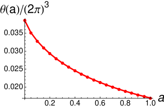
Figure 6: Second-order perturbative contribution at half filling $\vartheta(\pi/2,\pi/2,a)/(2\pi)^{3}$ for different values of $a$; solid line is a guide for the eye.

We will consider first the case when the density is medium-high: $n_{\uparrow}=n_{\downarrow}=n/2>0.25$, when a transition from HP to TSS state should always take place, being $\nu^{*}>n/2$ unfavored. By inspecting Eq. (9) it turns out that the ground state in the weak coupling limit is always homogeneous, even for large $z$ ($a<0.2$, i.e. $z>2/3$). This fact agrees with previous numerical results F2007 showing that the TSS phase is present only for $U/t_{\uparrow}\gtrsim 2.5$. Even close to quarter filling, the phase transition in the FK limit is predicted at $U/t_{\uparrow}=1.15$, which is beyond the weak coupling regime we are considering in this section.

Let us examine now the low density regime: $n_{\uparrow}=n_{\downarrow}=n/2<0.25$, where the TSS might be the ground state only at very small $a$. Now we have to determine the transition point from HP to TSS state in the FK limit ($a$ very small) as well as to explore the possibility of a transition to a PS state with $\nu>n_{\downarrow}$ for larger values of $a$. We will examine first the $n=1/3$ case as an example. In the highly asymmetric regime ($a<0.01$, i.e. $z>0.98$), we again find a transition from a HP to a TSS state which happens for values of $U(n=1/3)/t_{\uparrow}\sim 0.3$. As explained in the previous section, using Eqs. (3) and (4) we can determine the phase transition line between TSS and a PS state with $\nu\neq n_{\downarrow}$. This transition occurs for $t_{\downarrow}(n=1/3)/t_{\uparrow}\sim 0.025$, a value which turns out to be independent of $U$ since no contributions from the correlation energy are present. These transition points are in good accordance with the numerical results reported in F2007 , and allow us to complete a general weak coupling phase diagram in the highly asymmetric regime for $n=1/3$, which is shown in Fig. 7. At smaller densities, the critical value $U(n)/t_{\uparrow}$ at which one finds the transition from the HP to the TSS state becomes smaller. For example $U(n=1/6)/t_{\uparrow}\sim 0.06$, while $U(n=1/12)/t_{\uparrow}\lesssim 10^{-3}$. We notice that it is impossible, within our perturbative approach (see Eq. (9)), to find for this coefficient a value equal to zero: its value decreases as $n$ becomes smaller but stays always finite, going to zero smoothly as $n$ tends to zero. In addition, the TSS is always unstable with respect to a PS one, the transition now appearing at lower asymmetries ($t_{\downarrow}(n=1/6)/t_{\uparrow}\sim 2.5\times 10^{-3}$, $t_{\downarrow}(n=1/12)/t_{\uparrow}\sim 2.7\times 10^{-4}$), whose values are still essentially insensitive to $U$.

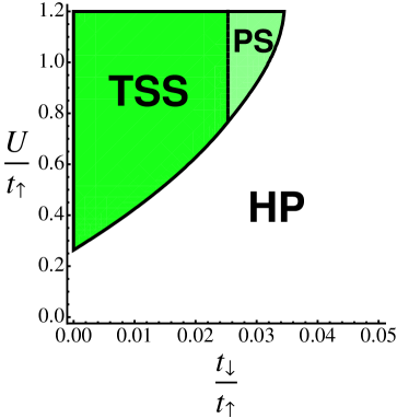
Figure 7: Weak-coupling phase diagram with $n=1/3$: white region represents the homogeneous state (HP), green regions are different phase separated states. The phase transition lines are computed using Eq. (4) (dashed) and Eq. (9) (solid). In this section we have adopted the parameters $U/t_{\uparrow}=u/(1+z)$ and $a=t_{\downarrow}/t_{\uparrow}=(1-z)/(1+z)$ instead of $u$ and $z$ to facilitate the comparison with previous results in the weak-coupling region.

IV Strong-coupling limit

In this section we analyze the case of strong repulsive onsite interaction between fermions, corresponding to $t_{\sigma}\ll U$, a regime which is of particular interest for the experimental realization of the symmetric ($z=0$) model in a cold atom system Jetal2008 , in which a Mott-insulator phase at half filling was found. One of the questions left open by bosonization is what happens to the HP-PS transition curve close to $z=0$. From the phase diagrams in refs. CHG2005 and M2007 it is not clear whether it approaches a finite value when $z\to 0$ or, conversely, if there is a characteristic value of $z\neq 0$ at which it diverges, as indicated also by some data on short sizes in ref. GFL2007 (Sec. IV therein). To study this regime, we will construct an effective Hamiltonian that is able to describe the AHM when the parameter $t$ can be considered as a small perturbation with respect to $U$, for a generic filling, by using the method of the flow equations, developed by Wegner W1994 and applied to the HM in S1997 . The advantages of using such a technique are extensively described in S1997 . We only remark here that it yields a very general procedure which, in a recursive way, allows to find an effective Hamiltonian at any order of perturbation, for arbitrary fillings and geometries.

We start by decomposing the fermionic Hilbert space of the model into the subspaces $\mathcal{H}_{k}$ with exactly $k$ fermionic pairs (double occupancies): $\mathcal{H}=\oplus_{k=0}^{N/2}\mathcal{H}_{k}$. The projectors $P_{k}$ on these subspaces are defined via the generating function

$$\sum_{k=0}^{N}P_{k}x^{k}=\prod_{i\in L}\left[1-(1-x)n_{i\uparrow}n_{i\downarrow}\right].$$

The kinetic energy term for the spin $\sigma$ fermions, $T_{\sigma}=\sum_{<ij>}c_{i\sigma}^{\dagger}c_{j\sigma}$, can be decomposed into three parts $T_{\sigma}=T_{0\sigma}+T_{+1\sigma}+T_{-1\sigma}$, which change the number of pairs by $\delta k=m=0,+1,-1$. In other words: $T_{m\sigma}=\sum_{k=0}^{N}P_{k+m}T_{\sigma}P_{k}$. In these expressions, we have introduced the sum over $<ij>$ which denotes nearest-neighbors sites $i$ and $j$ (with the couples $ij$ and $ji$ counted once each) since the procedure we are going to discuss is generalizable to any dimension. More explicitly:

$$T_{0\sigma}=\sum_{<ij>}\left[n_{i\bar{\sigma}}c_{i\sigma}^{\dagger}c_{j\sigma}n_{j\bar{\sigma}}+(1-n_{i\bar{\sigma}})c_{i\sigma}^{\dagger}c_{j\sigma}(1-n_{j\bar{\sigma}})\right]$$

$$T_{+1\sigma}=\sum_{<ij>}n_{i\bar{\sigma}}c_{i\sigma}^{\dagger}c_{j\sigma}(1-n_{j\bar{\sigma}})$$

$$T_{-1\sigma}=\sum_{<ij>}(1-n_{i\bar{\sigma}})c_{i\sigma}^{\dagger}c_{j\sigma}n_{j\bar{\sigma}}$$

It is not difficult to verify that $\left[N_{d},T_{m\sigma}\right]=mT_{m\sigma}$, where $N_{d}=\sum_{i}n_{i\uparrow}n_{i\downarrow}$, reflecting the transition from the Hilbert space $\mathcal{H}_{k}$ to $\mathcal{H}_{k+m}$. To discuss higher-order interactions terms, it is useful to introduce products of hopping operators, $T_{\sigma_{1}\dots\sigma_{k}}^{(k)}(\mathbf{m})=T_{m_{1}\sigma_{1}}...T_{m_{k}\sigma_{k}}$ with the index vector $\mathbf{m}=(m_{1},m_{2},...,m_{k})$. It is found that the commutator of such an operator product with $N_{d}$ involves the total weight of the product, $M(\textbf{m})=\sum_{i=1}^{k}m_{i}$, and generally reads $\left[N_{d},T_{\sigma_{1}\dots\sigma_{k}}^{(k)}(\mathbf{m})\right]=M(\mathbf{m})T_{\sigma_{1}\dots\sigma_{k}}^{(k)}(\textbf{m})$. We want now to find an effective Hamiltonian which does not mix the different Hilbert space sectors $\mathcal{H}_{k}$, i.e. which conserves the total number of local pairs, thus suited to study physical properties at energy and temperature scales which are well below the Hubbard energy $|U|$. To do so, we consider a continuous unitary transformation which allows to remove interactions with non-vanishing overlap between different Hilbert space sectors. Thus, the transformed Hamiltonian depends on a continuous flow parameter $l$:

$$H(l)=-\sum_{\sigma}t_{\sigma}\Theta_{\sigma}(l)+UN_{d}$$

where the generalized kinetic energy term $\Theta_{\sigma}(l)$ contains all order interactions which are generated by the transformation:

$$\Theta_{\sigma}(l)=\sum_{k=1}^{\infty}\frac{t_{\sigma}^{k-1}}{U^{k-1}}\sum_{\{\mathbf{m}\}}F_{\sigma_{1}...\sigma_{k}}^{(k)}(l;\mathbf{m})T_{\sigma_{1}...\sigma_{k}}^{(k)}(\mathbf{m})$$ (10)

Here $F_{\sigma_{1}...\sigma_{k}}^{(k)}$ denote suitable coupling functions that have to be determined by asking that the unitary transformation cancels all terms that do not conserve the number of local pairs. The flow equations for these coupling functions follow from the equation of the flow for the Hamiltonian W1994 :

$$\frac{dH(l)}{dl}=\left[\eta_{\sigma}(l),H(l)\right]$$ (11)

which has been written here by using the (antihermitean) generator of the transformation

$$\eta_{\sigma}(l)=\frac{t_{\sigma}}{U}\left[V,\Theta_{\sigma}(l)\right]=$$

$$=\sum_{k=1}^{\infty}\frac{t_{\sigma}^{k}}{U^{k}}\sum_{\{\mathbf{m}\}}M(\mathbf{m})F_{\sigma_{1}...\sigma_{k}}^{(k)}(l;\mathbf{m})T_{\sigma_{1}...\sigma_{k}}^{(k)}(\mathbf{m})$$

Now, after imposing both the initial conditions ($F_{\sigma_{1}}^{(1)}(0;m)=1$ and $F_{\sigma_{1}\dots\sigma_{k}}^{(k)}(0;\textbf{m})=0$ for $k>1$) and the symmetries related to hermiticity and particle-hole transformation $c_{i\sigma}^{\dagger}\rightarrow c_{i\sigma}$, which reverses the sign of the hopping term, one can recast the original flow equation (11) in a recursive set of coupled nonlinear differential equations. From these equations it is easy to see that all the terms which connect different sectors of the Hilbert space vanish in the limit $l\rightarrow\infty$. At the second order we find that the effective Hamiltonian reads

$$H_{s-c}=-t_{\uparrow}\sum_{<ij>}\Big{[}n_{i\downarrow}c_{i\uparrow}^{\dagger}c_{j\uparrow}n_{j\downarrow}+(1-n_{i\downarrow})c_{i\uparrow}^{\dagger}c_{j\uparrow}(1-n_{j\downarrow})\Big{]}$$

$$-t_{\downarrow}\sum_{<ij>}\Big{[}n_{i\uparrow}c_{i\downarrow}^{\dagger}c_{j\downarrow}n_{j\uparrow}+(1-n_{i\uparrow})c_{i\downarrow}^{\dagger}c_{j\downarrow}(1-n_{j\uparrow})\Big{]}$$

$$+J\sum_{<ij>}\Big{[}S_{i}^{x}S_{j}^{x}+S_{i}^{y}S_{j}^{y}+\Delta(S_{i}^{z}S_{j}^{z}-n_{i}n_{j}/4)\Big{]}+UN_{d}$$ (12)

where $S_{i}^{x,y,z}$ are the spin operators at site $i$, $J=2t_{\uparrow}t_{\downarrow}/U$ and $\Delta=(t_{\uparrow}^{2}+t_{\downarrow}^{2})/2t_{\uparrow}t_{\downarrow}\geq 1$. At half filling, $n=1$, we get, according to the Takahasi’s theorem T1977 , that the terms corresponding to the odd orders of the expansion (in the our case the first two lines) vanish and we find the same Hamiltonian obtained in FDL1995 representing a spin chain with an anisotropy term $\Delta\geq 1$ along the $z-$axis (XXZ chain): the spin excitations are gapped and the spin-spin correlators decay exponentially with the distance. Also, in the limit $t_{\uparrow}=t_{\downarrow}$ (symmetric HM) the anisotropy term $\Delta$ becomes 1 and we find the well-known Heisenberg Hamiltonian (XXX chain), as it should be.

It is well known FDL1995 that for $z>0$ the system is in the Néel-like phase, with non-vanishing charge and spin gap and true long-range order. Here we are interested in examining the two limiting cases $z=1$ (FK model) and $z=0$ (Hubbard model) to study, more precisely, $(i)$ the phase appearing in the Hubbard model when $U\rightarrow\infty$, i.e. the so called spinless fermions phase (SF), where the orientation of the spins loses its relevance since the doubly occupied sites are strictly forbidden, and $(ii)$ the state predicted in the FK model where the two fermionic species are demixed.

IV.1 Spinless fermions

The SF state $|\Psi\rangle_{SF}$ of the Hubbard model in the limit $U\to\infty$ at filling $n=N/L\leq 1$ and equally populated species $n_{\uparrow}=n_{\downarrow}=n/2$ is rotationally invariant and invariant under the up-down exchange. In this case, the expectation value of the hopping terms of the Hamiltonian (12) reads as follows

$${}_{SF}\langle\Psi|[-t\sum_{j,\sigma}(c_{j\sigma}^{\dagger}c_{j+1\sigma}+{\rm h.c.})-tz\sum_{j}(c_{j\uparrow}^{\dagger}c_{j+1\uparrow}+{\rm h.c.})$$

$$+tz\sum_{j}(c_{j\downarrow}^{\dagger}c_{j+1\downarrow}+{\rm h.c.})]|\Psi\rangle_{SF}=-\frac{2t}{\pi}\sin(\pi n)$$

As for the $J$-terms, we can borrow directly its expression from (A3) of OS1990 :

$$\frac{{}_{SF}\langle\Psi|\sum_{j}n_{j}n_{j+1}|\Psi\rangle_{SF}}{L}=n^{2}-\frac{\sin^{2}(\pi n)}{\pi^{2}}$$ (13)

Moreover, since $|\Psi\rangle_{SF}$ is SU(2)-invariant, we can write

$$\frac{{}_{SF}\langle\Psi|\sum_{j}S_{j}^{\alpha}S_{j+1}^{\alpha}|\Psi\rangle_{SF}}{L}=\frac{1}{3}\frac{{}_{SF}\langle\Psi|\sum_{j}\vec{S}_{j}\cdot\vec{S}_{j+1}|\Psi\rangle_{SF}}{L}$$ (14)

for $\alpha=x,y,z$ even if the $J$-part in the strong-coupling Hamiltonian is anisotropic, where now, from (A3) and (A4) of of OS1990 , we find

$$\frac{{}_{SF}\langle\Psi|\sum_{j}\vec{S}_{j}\cdot\vec{S}_{j+1}|\Psi\rangle_{SF}}{L}=\left(\frac{1}{4}-\ln 2\right)\left[n^{2}-\frac{\sin^{2}(\pi n)}{\pi^{2}}\right].$$

Collecting all the pieces it is easy to see that

$${\cal{\cal E}}_{SF}=\frac{{}_{SF}\langle\Psi|H_{s-c}|\Psi\rangle_{SF}}{L}=-\frac{2t}{\pi}\sin(\pi n)+$$

$$+\frac{4t^{2}(1-z^{2})}{U}\left[n^{2}-\frac{\sin^{2}(\pi n)}{\pi^{2}}\right]\left[\frac{2+\Delta}{3}\left(-\ln 2+\frac{1}{4}\right)-\frac{1}{4}\right]$$

As an example, in Fig. 8 we plot the local densities of fermions obtained numerically on a chain with $L=60$ and open boundary conditions (OBC), $z=0.1$, $n=0.2$ and $u=100$. The two species tend to occupy alternate regions but the fraction of double occupation is still significant. The comparison with the total density profile for spinless fermions at the same equivalent filling shows that the SF state is a good description of the ground state in this case. We have verified that the same happens if the filling is increased up to $n=0.9$, the other parameters being unchanged. On the contrary, if we still fix $u=100$, $n=0.2$ but increase the anisotropy to $z=0.3$, appreciable differences in the density profiles start to appear.

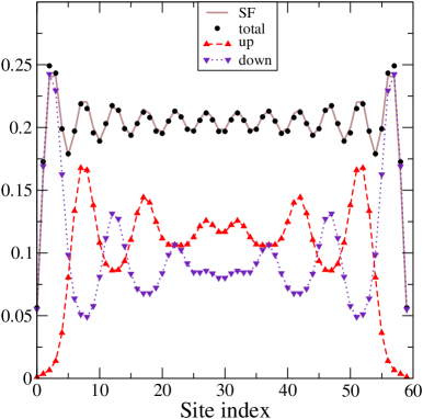
Figure 8: Spatial density profiles for an open chain with $z=0.1$, filling $n=0.2$ and $u=100$. The continuous curve labelled SF is the local density for an equivalent chain of spinless fermions (i.e. Eq. (17) with $\ell=L$ and $p=nL)$, showing a very good agreement with the spinful numerical data.

IV.2 Spatially separated states

In the strong-coupling approach we can actually formulate a slightly more general form of the PS state with respect to that of Sec. III.1 which, however, leads formally to the same analytical expressions. Let us consider a sequence of $M$ contiguous intervals $I_{j\uparrow}$, $I_{j\downarrow}$ ($j=1,\dots,M$) and a state $|\Psi\rangle_{PS}$ in which the up and down spins are separated in the sense that there are no doubly occupied sites, $I_{1\uparrow}$ contains only up spins, $I_{1\downarrow}$ contains only down spins, then again $I_{2\uparrow}$ with up spins and so on. Let $L_{j\sigma}$ and $N_{j\sigma}$, respectively, the number of sites and the number of electrons in the interval $I_{j\sigma}$. We then make the further strong assumption that each up or down interval, irrespective of its length, is equally filled meaning that $\bar{n}_{\uparrow}=N_{j\uparrow}/L_{j\uparrow}$ and $\bar{n}_{\downarrow}=N_{j\downarrow}/L_{j\downarrow}$ do not depend on $j$. Now, if

$$\nu L=\sum_{j=1}^{M}L_{j\downarrow}\;,\;\;(1-\nu)L=\sum_{j=1}^{M}L_{j\uparrow}$$

are the total lengths associated with the motion of down and up spins we have $N_{\uparrow}=\sum_{j=}^{M}N_{j\uparrow}=\sum_{j=1}^{M}\bar{n}_{\uparrow}L_{j\uparrow}=\bar{n}_{\uparrow}L(1-\nu)$ and similarly $N_{\downarrow}=\bar{n}_{\downarrow}L\nu$ and so, for equally populated species $\bar{n}_{\uparrow}=n/[2(1-\nu)]$ and $\bar{n}_{\downarrow}=n/(2\nu)$.

We first consider the thermodynamic limit in the case in which the interface points (which are $2M$ in number) do not contribute to the bulk energy density ($\lim_{L\to\infty}2M/L=0$) and, at the same time, each interval is extensively large ( $\lim_{L\to\infty}L_{j\sigma}/L>0$), so that for every interval we can use the formula for the kinetic energy density of free fermions without worrying about finite-size and/or boundary effects:

$$\frac{{}_{PS}\langle\Psi|T_{s-c}|\Psi\rangle_{PS}}{L}=\frac{\sum_{j=1}^{M}L_{j\uparrow}}{L}\left[-\frac{2t_{\uparrow}}{\pi}\sin\left(\pi\frac{n}{2(1-\nu)}\right)\right]$$

$$+\frac{\sum_{j=1}^{M}L_{j\downarrow}}{L}\left[-\frac{2t_{\downarrow}}{\pi}\sin\left(\pi\frac{n}{2\nu}\right)\right]$$

$$=-\frac{2t_{\uparrow}}{\pi}(1-\nu)\sin\left(\pi\frac{n}{2(1-\nu)}\right)-\frac{2t_{\downarrow}}{\pi}\nu\sin\left(\pi\frac{n}{2\nu}\right).$$

Note that we do not necessarily require that the heavy (down) species is fully compressed, meaning $\nu=n/2$. The value for $\nu$ will be determined variationally in order to give the smallest possible energy at a fixed $z$, exactly as done in Sec. III.2. Let us now calculate the energy of such a state.

As far as the $J$-term is concerned we first note that the transverse part is vanishing. In fact both $S_{j}^{x}$ and $S_{j}^{y}$ are composed by spin-flip terms like $c_{j\sigma}^{\dagger}c_{j\bar{\sigma}}$ but each interval contains spins of only one specie. Next, all the $\Delta$-term can be rewritten as

$$\Delta\left(S_{j}^{z}S_{j+1}^{z}-\frac{n_{j}n_{j+1}}{4}\right)=\frac{\Delta}{4}[(n_{j\uparrow}-n_{j\downarrow})(n_{j+1\uparrow}-n_{j+1\downarrow})$$

$$-(n_{j\uparrow}+n_{j\downarrow})((n_{j+1\uparrow}+n_{j+1\downarrow})]=-\frac{\Delta}{2}(n_{j\uparrow}n_{j+1\downarrow}+n_{j\downarrow}n_{j+1\uparrow}).$$ (15)

When the expectation value on $|\Psi\rangle_{PS}$ is taken, the up and down parts factorize and there can be non-vanishing contributions only when $j$ and $j+1$ are at an interface between two intervals carrying opposite spins. If, as assumed above, the number of interface points does not grow as $L$ we can neglect these contributions in the limit $L\to\infty$. Therefore the energy density of the PS state reads

$${\cal E}_{PS}(\nu)=\frac{{}_{PS}\langle\Psi|H_{s-c}|\Psi\rangle_{PS}}{L}$$

$$=-\frac{2t_{\uparrow}}{\pi}(1-\nu)\sin\left(\pi\frac{n}{2(1-\nu)}\right)-\frac{2t_{\downarrow}}{\pi}\nu\sin\left(\pi\frac{n}{2\nu}\right).$$

As anticipated, this expression coincides with Eq. (3) in the balanced case $n_{\uparrow}=n_{\downarrow}=n/2$. In Fig. 9 we present two examples of the spatial density profile for large $u$ and intermediate/large $z$, from which the spatial separation of the two species can be clearly inferred. Note also that the light specie occupies regions with a non-vanishing fraction of empty sites and an oscillating density profile $\langle n_{j\uparrow}\rangle$ is seen. Nonetheless the local density in the intervals occupied by the heavy fermions does not reach 1, so in these case we do not have a TSS as instead, for example, in Fig. 3 of ref. S-VFF2007 valid for $u=20$, $z=2/3$, filling $n=0.8$ on 40 sites (reproduced in our calculations but not shown here).

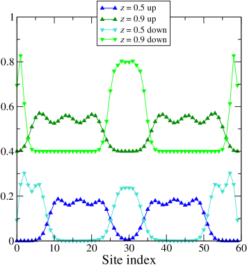
Figure 9: Spatial density profiles for open chains with $z=0.5$ and $z=0.9$ (offset by $+0.4$ for clarity), filling $n=0.2$ and $u=100$.

IV.3 PS’: Extensive number of intervals $M=\alpha L$

In order to treat also the case in which the number of interfaces scales as a finite fraction $\alpha$ of the total number of sites, we will assume that all the intervals hosting up spins are equally long and equally filled: $L_{j\uparrow}=\ell_{\uparrow}$, $N_{j\uparrow}=p_{\uparrow}$ $\forall j=1,\dots,M$ so that $\ell_{\uparrow}=(1-\nu)/\alpha$ and $p_{\uparrow}=n/(2\alpha)$; similarly for the intervals with down spins $\ell_{\downarrow}=\nu/\alpha$ and $p_{\downarrow}=n/(2\alpha)=p_{\uparrow}$. Note that, for equally populated species, necessarily the finite number of electrons in each interval is the same for up or down spins, while the finite lengths are in general different. The energy density of this type of phase separated state will therefore have the form

$${\cal E}_{PS^{\prime}}=\frac{M}{L}(\kappa_{\uparrow}+\kappa_{\downarrow})-\frac{J\Delta}{L}\sum_{j=1}^{L}(\langle n_{j\uparrow}\rangle\langle n_{j+1\downarrow}\rangle+\langle n_{j\downarrow}\rangle\langle n_{j+1\uparrow}\rangle)$$

where $\kappa_{\uparrow,\downarrow}$ are the kinetic energies of $p=p_{\uparrow}=p_{\downarrow}$ up or down fermions on intervals of length $\ell_{\uparrow,\downarrow}$ with OBC, while the $\Delta$-term comes from Eq. (15) and now cannot be neglected. The on-site terms $\langle n_{j\sigma}\rangle$ also have to be evaluated in the same fashion and will be localized at the left or right end of the intervals (with equal values). Let us denote them by $\eta_{\sigma}$; we have a contribution $\langle n_{{\rm right}\uparrow}\rangle\langle n_{{\rm left}\downarrow}\rangle+\langle n_{{\rm right}\downarrow}\rangle\langle n_{{\rm left}\uparrow}\rangle=2\eta_{\uparrow}\eta_{\downarrow}$ for each of the $M$ pairs of up+down intervals so that

$${\cal E}_{PS^{\prime}}=\alpha(\kappa_{\uparrow}+\kappa_{\downarrow}-2J\Delta\eta_{\uparrow}\eta_{\downarrow}).$$

The calculation of the kinetic energy and of the surface density for an effective open chain of $\ell$ sites with $p$ free fermions is given in the appendix, leading to:

$${\cal E}_{PS^{\prime}}=\alpha t\{(1+z)\left\{1-\frac{\sin\left[\frac{\pi(2p+1)}{2(\ell_{\uparrow}+1)}\right]}{\sin\left[\frac{\pi}{2(\ell_{\uparrow}+1)}\right]}\right\}$$

$$+(1-z)\left\{1-\frac{\sin\left[\frac{\pi(2p+1)}{2(\ell_{\downarrow}+1)}\right]}{\sin\left[\frac{\pi}{2(\ell_{\downarrow}+1)}\right]}\right\}$$

$$-\frac{1+z^{2}}{u}\frac{\left\{2p+1-\frac{\sin\left[\frac{\pi(2p+1)}{\ell_{\uparrow}+1}\right]}{\sin\left(\frac{\pi}{\ell_{\uparrow}+1}\right)}\right\}\left\{2p+1-\frac{\sin\left[\frac{\pi(2p+1)}{\ell_{\downarrow}+1}\right]}{\sin\left(\frac{\pi}{\ell_{\downarrow}+1}\right)}\right\}}{(\ell_{\uparrow}+1)(\ell_{\downarrow}+1)}\}.$$

The conditions $p\leq\ell_{\uparrow}$ and $p\leq\ell_{\downarrow}$ define the range of $\nu\in[n/2,1-n/2]$, while the conditions $p\geq 1$, $\ell_{\uparrow}\geq 1$ and $\ell_{\downarrow}\geq 1$ imply $\alpha\leq\min(n/2,\nu,1-\nu)=n/2$. Once this expression is minimized by suitable values of $\alpha$ and $\nu$ in this range we should, at least, check if the resulting energy density is smaller than the optimal energy density ${\cal E}_{PS}$ determined above for the same values of $z$, $n$ and, now, also $u$.

Finally, we mention that we have also tried to enlarge the set of trial/variational states by including the homogeneous one (defined in Sec. III), which is the correct ground state in the limit $U=0$ for all $z$. However we have verified that this additional state, for the fillings we have considered, could become relevant only when $u\lesssim 1$, outside the domain of validity of the strong-coupling approach. Therefore, for the sake of compactness, we do not report these results here.

IV.4 Phase boundaries

From the condition ${\cal E}_{PS}<{\cal E}_{SF}$ we get

$$-\frac{2(1+z)}{\pi}(1-\nu^{*})\sin\left(\pi\frac{n}{2(1-\nu^{*})}\right)$$

$$-\frac{2(1-z)}{\pi}\nu^{*}\sin\left(\pi\frac{n}{2\nu^{*}}\right)<-\frac{2}{\pi}\sin(\pi n)$$

$$+\frac{4(1-z^{2})}{u}\left[n^{2}-\frac{\sin^{2}(\pi n)}{\pi^{2}}\right]\left[\frac{2+\Delta}{3}\left(-\ln 2+\frac{1}{4}\right)-\frac{1}{4}\right]$$

that is $u<u_{PS}(z)$ for $d(n,z)>0$ or $u>u_{PS}(z)$ otherwise, having defined

$$d(n,z)=\sin(\pi n)-(1+z)(1-\nu^{*})\sin\left[\pi\frac{n}{2(1-\nu^{*})}\right]$$

$$-(1-z)\nu^{*}\sin\left(\pi\frac{n}{2\nu^{*}}\right)$$

and

$$u_{PS}(n,z)=2\pi(1-z^{2})\frac{\left[n^{2}-\frac{\sin^{2}(\pi n)}{\pi^{2}}\right]\left[\frac{2+\Delta}{3}\left(-\ln 2+\frac{1}{4}\right)-\frac{1}{4}\right]}{d(n,z)}$$

Now we can draw a phase diagram in the $(z,u)$-plane for a fixed value of the total filling $n$ by indicating the regions where the PS or the SF state has the lower energy. We show two examples (for $n=0.4$ and $0.9$) in Figs. 10 and 11, respectively. We have analyzed in detail also the phase diagram for $n=0.6$ (not shown), that turns out be qualitatively similar to the one for $n=0.4$. Having in mind that bosonization could be considered quantitatively reliable only for small values of the interaction, we have reported in the figures (dashed lines) the curves of Wentzel-Bardeen instability M2007 where the velocity of one of the bosonization modes vanishes thereby indicating phase separation. In addition, we have considered two typical cases of PS at $n=0.9$ $(L=20,40,60)$, namely those at $u=100$ for $z=0.1$ and at $u=5$ for $z=0.9$. In both cases, the charge structure factor $S(q)$ (as defined in Sec. II) displays a divergence for $q\to 0$ typical of PS states SBC2004 and a peak at $q=4k_{F}({\rm mod}2\pi)=2\pi n({\rm mod}2\pi)=2\pi(1-n)$.

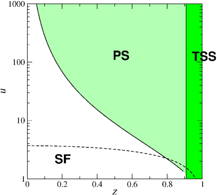
Figure 10: Transition lines in the $(z,u)$-plane at filling $n=0.4$ indicating how the ground state changes from SF to PS. In the separated regime above the transition lines, the state can be either PS (left) or TSS (right) (see Sec. III.2) and the edge between the two is marked by a vertical line (analogously to Fig. 3 of ref. F2007 ). The dashed line corresponds to the bosonization prediction.

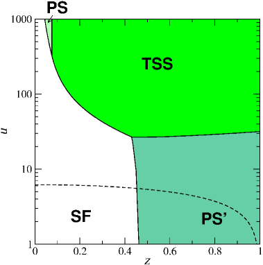
Figure 11: Same as Fig. 10 but with filling $n=0.9$. Now also the PS’ (see text) state is relevant for moderate values of $u$ and the corresponding transition lines with SF and PS are marked.

In the strong-coupling approach the most interesting thing to understand seems to be the divergence of the transition line separating PS from SF behaviour at small $z$ and large $u$. We have verified that when $\nu=\nu^{*}(z)$ is inserted into $d(n,z)$ the denominator appearing in $u_{PS}(n,z)$ is always negative. In order to estimate $u_{PS}(n,z)$ analytically we set $\nu^{*}(z)=1/2-z\nu_{1}-z^{2}\nu_{2}+O(z^{3})$ with $\nu_{1,2}>0$ (see Fig. 4) and expand $d(n,z)$ for $z\to 0$

$$d(n,z)=-2\nu_{1}[f(\pi n)-\pi^{2}n^{2}\nu_{1}\sin(\pi n)]z^{2}+O(z^{3})$$

so that at leading order

$$u_{PS}(n,z)=\frac{1}{z^{2}}\frac{\pi\ln 2\left[n^{2}-\frac{\sin^{2}(\pi n)}{\pi^{2}}\right][1+O(z)]}{\nu_{1}(n)[f(\pi n)-\pi^{2}n^{2}\nu_{1}(n)\sin(\pi n)]}$$ (16)

with $f(x)=\sin x-x\cos x$ as before. As far $\nu_{1}(n)$ as is concerned, by inserting $\nu=1/2-z\nu_{1}+O(z^{2})$ in Eq. (5) and solving at first order in $z$ we get $\nu_{1}(n)=f(\pi n)/[f^{\prime}(\pi n)2\pi n]$. In summary, our analytical approach predicts that there is no finite value of $z$ below which PS disappears; by moving to a sufficiently large repulsive coupling it is always possible to induce a PS at arbitrarily small anisotropy.

IV.5 Inclusion of phase separated states with an infinite number of interfaces

We have compared the energy density of the PS state at given values of $n$ and $z$ with the corresponding value for the PS’ state discussed in Sec. IV.3. At small filling, say $n=0.1$, the two variational solutions (with respect to $\nu$ or $\nu$ and $\alpha$, respectively) coincide in the sense that the optimal value $\alpha^{*}\to 0$ and the optimal value of $\nu$ is the same. Moreover ${\cal E}_{PS^{\prime}}\geq{\cal E}_{PS}$. When the filling is increased to, say, $n=0.4$ the situation is similar with the exception of a small region ($u\lesssim 0.8$ for $z=0$ or $u\lesssim 2.8$ for $z=0.9$) that can be considered to be outside the scope of the strong-coupling approach. At $n=0.6$, the PS’ solution can be ignored for $u\gtrsim 3.2$ (a result checked at $z=0$ and $z=0.1$) or $u\gtrsim 5.2$ (as checked at $z=0.5$ and $z=0.9)$. Thus, close to half-filling the PS’ becomes relevant also at intermediate values of $u$ and we have examined it in more detail.

Let us fix $n=0.9$; in the symmetric case $z=0$ the optimal value of $\alpha$ remains at its maximum $\alpha^{*}=n/2$ for $u<32$ where it starts to decrease to reach $\alpha^{*}=0$ at $u\cong 44.3$; the PS’ state has a lower energy density with respect to the PS one for $u\lesssim 45.8$. For positive $z$ as long as $z\leq 0.43$ the PS’ solution is never better than the ones considered before. When $z$ increases further the PS’ state is favored over the PS or even the SF one; the region at large $z$ and moderate $u$ where $|\Psi\rangle_{PS^{\prime}}$ has a lower energy is characterized by the fact that $\alpha^{*}=n/2$ and $\nu^{*}=n/2$ so that $p=\ell_{\downarrow}=1$ meaning that all the down spins are isolated from each other. This configuration resembles the trimer crystal phase found in ref. KCR2009 , with a mixture of hardcore bosons with attractive interaction and fillings 1/3 and 2/3, which is equivalent to a repulsive case with balanced species and total filling 2/3 when a particle-hole transformation is performed.

V Conclusions

Our study, which combines analytical calculations in the strong- and weak-coupling regimes and DMRG simulations both for attractive and repulsive interaction, sheds some light on three qualitative and quantitative questions that are still open in the literature of the 1D AHM:

1. The shape of the transition line from SS to CDW dominant correlations for $U<0$ is filling-dependent and re-entrant in some cases (see Fig. 3);

2. Phase separation and phase segregation take place close to the Falicov-Kimball limit above an interaction value $U_{c}$ which depends on the population in such a way that it approaches zero in the small density regime. Furthermore, transitions between phase separation and phase segregation at varying interaction take place at a nearly constant asymmetry;

3. For small asymmetry, close to the Hubbard limit $t_{\downarrow}\lesssim t_{\uparrow}$, the SF-PS transition takes place at larger and larger values of $U$; Eq. (16), obtained in the framework of a variational strong-coupling argument, indicates that an arbitrarily small asymmetry is sufficient, at very large repulsions, to create a phase separated state which destroys the spinless fermion-like ground state of the Hubbard model.

Appendix: Free spinless fermions with open boundary conditions

The eigenfunctions of the hopping operator $-t\sum_{j=1}^{L-2}(c_{j}^{\dagger}c_{j+1}+{\rm h.c.})$ have the form

$$\varphi_{m}(j)=\sqrt{\frac{2}{\ell+1}}\sin(k_{m}j)\;,\;\;k_{m}=\frac{\pi m}{\ell+1}\;,\;\;m=1,\dots,\ell$$

and the dispersion relation is formally the same as in the case of PBC $\epsilon(k_{m})=-2t\cos(k_{m})$ so

$$\kappa=-2t\sum_{m=1}^{p}\cos\left(\frac{\pi m}{\ell+1}\right)=t\left\{1-\frac{\sin\left[\frac{\pi(2p+1)}{2(\ell+1)}\right]}{\sin\left[\frac{\pi}{2(\ell+1)}\right]}\right\}$$

where $p\leq\ell$ is the number of particles.

To compute the average density on the $j$-th site $\langle n_{j}\rangle$ we pass to the creation/annihilation operators in $k$-space

$$c_{j}=\sqrt{\frac{2}{L+1}}\sum_{m=1}^{\ell}\sin\left(\frac{\pi m}{\ell+1}j\right)\tilde{c}_{k_{m}}$$

$$\langle n_{j}\rangle=\frac{2}{L+1}\sum_{m,m^{\prime}}\sin\left(\frac{\pi m}{\ell+1}j\right)\sin\left(\frac{\pi m^{\prime}}{\ell+1}j\right)\times$$

$$\times\langle 0|\tilde{c}_{k_{1}}\dots\tilde{c}_{k_{p}}(\tilde{c}_{k_{m}}^{\dagger}\tilde{c}_{k_{m^{\prime}}})\tilde{c}_{k_{p}}^{\dagger}\dots\tilde{c}_{k_{1}}^{\dagger}|0\rangle$$

The only non-vanishing possibility within the matrix element for the vacuum $|0\rangle$ filled up to the momentum $k_{p}=\pi p/(\ell+1)$ is $m^{\prime}=m$, so we have the characteristic function of the Fermi sea $n_{k_{m}}$

$$\langle n_{j}\rangle=\frac{2}{\ell+1}\sum_{m=1}^{p}\sin^{2}\left(\frac{\pi m}{\ell+1}j\right)$$

$$=\frac{p}{\ell+1}-\frac{1}{\ell+1}\sum_{m=1}^{p}\cos\left(\frac{2\pi m}{\ell+1}j\right)$$

$$=\frac{2p+1}{2(\ell+1)}-\frac{\sin\left[\frac{\pi(2p+1)}{\ell+1}j\right]}{2(\ell+1)\sin\left(\frac{\pi}{\ell+1}j\right)}$$ (17)

The density at the edge is obtained by setting $j=1$.

References

- (1) M. A. Cazalilla, A. F. Ho, T. Giamarchi, Phys. Rev. Lett. 95, 226402 (2005)
- (2) B. Wang, H.-D. Chen, S. Das Sarma, Phys. Rev. A 79, 051604(R) (2009)
- (3) G. G. Batrouni, M. J. Wolak, F. Hébert, V. G. Rousseau, Europhys. Lett. 86, 47006 (2009)
- (4) W. V. Liu, F. Wilczek, P. Zoller, Phys. Rev. A 70, 033603 (2004)
- (5) T. Giamarchi, Quantum physics in one dimension (Clarendon Press, Oxford, 2003)
- (6) L. M. Falicov, J. C. Kimball, Phys. Rev. Lett. 22, 997 (1969)
- (7) D. Ueltschi, J. Stat. Phys. 116, 681 (2004)
- (8) S. R. White, Phys. Rev. Lett. 69, 2863 (1992)
- (9) E. H. Lieb, F. Y. Wu, Phys. Rev. Lett. 20, 1445 (1968)
- (10) J. K. Freericks, E. H. Lieb, D. Ueltschi, Phys. Rev. Lett. 88, 106401 (2002)
- (11) Z. G. Wang, Y. G. Chen, S. J. Gu, Phys. Rev. B 75, 165111 (2007)
- (12) A. W. Sandvik, L. Balents, D. K. Campbell, Phys. Rev. Lett. 92, 236401 (2004)
- (13) L. Mathey, Phys. Rev. B 75, 144510 (2007)
- (14) Z. Domański, R. Łyżwa, P. Erdős, J. Mag. Mag. Mat. 140-144, 1205 (1995)
- (15) M. Ogata, H. Shiba, Phys. Rev. B 41, 2326 (1990)
- (16) Z. Domański, R. Lemanński, G. Fáth, J. Phys.: Condens. Matter 8, L261 (1996)
- (17) R. Jordens et al., Nature 455, 204 (2008)
- (18) F. Wegner, Ann. Phys. (Berlin) 3 (or 506), 77 (1994)
- (19) J. Stein, J. Stat. Phys. 88, 487 (1997)
- (20) M. Takahashi, J. Phys. C 10, 1289 (1977)
- (21) G. Fáth, Z. Domański, R. Lemański, Phys. Rev. B 52, 13910 (1995)
- (22) P. Farkašovský, Phys. Rev. B 77, 085110 (2007)
- (23) S.-J. Gu, R. Fan, H.-Q. Lin, Phys. Rev. B 76, 125107 (2007)
- (24) I. Bloch, J. Dalibard, W. Zwerger, Rev. Mod. Phys. 80, 885 (2008)
- (25) D. Jaksch et al., Phys. Rev. Lett. 81, 3108 (1998)
- (26) W.L. Chan et al., J. Phys.: Condens. Matter 20, 345217 (2008)
- (27) W. Metzner, D. Vollhardt, Phys. Rev. B 39, 7, 4462 (1989)
- (28) J. Silva-Valencia, R. Franco, M. S. Figueira, Physica B 398, 427 (2007)
- (29) W. H. Press, B. P. Flannery, S. A. Teukolsky, W. T. Vetterling, Numerical recipes in C, the art of scientific computing, Second edition (Cambridge University Press, 1992)
- (30) T. Keilmann, I. Cirac, T. Roscilde, Phys. Rev. Lett. 102, 255304 (2009)