Numerical investigations of the three-dimensional proton-proton screened Coulomb t-matrix

Abstract

We demonstrate behaviour of the momentum space screened Coulomb t-matrix, obtained by a numerical solution of the three-dimensional Lippmann-Schwinger equation. Examples are given for different types of screening. They prove that it is possible to obtain numerically a reliable three-dimensional screened Coulomb t-matrix, what is important in view of its application in few-body calculations.

I Introduction

The few nucleon systems can be nowadays studied using realistic nuclear forces in all their complexity. However, addition of the Coulomb force acting between protons poses serious obstacle and is still a challenging task. Up to now the long range Coulomb potential could be exactly implemented only into calculations of ³He and ⁴He bound states and of scattering states up to three nucleons.

In the proton-proton (pp) elastic scattering Coulomb force can be included exactly and observables can be calculated using e.g. the Vincent-Phatak method  Vincent74 . For three-nucleon (3N) reactions it is possible to include the Coulomb force when performing calculations of the elastic proton-deuteron (pd) scattering both in a coordinate kievski as well as in a momentum space representation deltuva ; witala . The pd breakup observables can be predicted only in the momentum space using two approaches deltuva2 ; witala2 . Both rely on the screened Coulomb potential and renormalization, what permits to apply standard methods valid for short-range interactions.

In the formalism of Refs. witala and witala2 the Coulomb interaction enters Faddeev equations via the screened Coulomb t-matrix. This t-matrix appears in a partial wave decomposed form as well as in its direct three-dimensional form for which no partial wave decomposition is performed. This allows to include the full Coulomb interaction, not restricted to the finite number of the lowest partial waves. Since that three-dimensional screened Coulomb t-matrix is a basic component of that formulation, therefore one has to put a special attention to its numerical realization.

Precise numerical calculations of the three dimensional screened Coulomb t-matrix are possible for any type of screening. They are numerically quite demanding but in principle use the concepts developed in elster1998 for the Malfliet-Tjion potential. This potential consists of two terms which have the same functional form as an exponentially screened Coulomb potential with the screening parameter $n=1$ (for details see below). Such particular value of the screening parameter $n$ allows one to perform many steps analytically when obtaining momentum space partial wave decomposed as well as direct three-dimensional t-matrix elements. The analogous procedure can be adapted to the higher values of $n$, as done in skib09 , where observables for pp scattering were calculated. Also there on-, half- and off-the-energy-shell elements of the t-matrix are compared with the analytical expressions in the screening limit from Refs. kok81 ; henrybook .

In this paper we present details of three-dimensional screened Coulomb t-matrix calculations. The behaviour of the numerically obtained t-matrix and its dependence on the screening parameters for different types of screening will be presented. In Sect.II we describe the numerical procedure to get the three dimensional screened Coulomb t-matrix. In Sect.III the behaviour of resulting t-matrices obtained with different forms of screening will be presented and t-matrices will be compared to the screened Coulomb potential. In Sect.IV the convergence of the partial wave decomposition of the screened Coulomb t-matrix will be shown by comparing it with the generated three-dimensional screened Coulomb t-matrix. Finally, we summarize in Sect.V.

II Numerical calculation of the screened Coulomb t-matrix.

The three-dimensional momentum space matrix elements of the screened Coulomb potential $<\vec{p}~{}^{\prime}|V_{c}^{R}|\vec{p}>\equiv V_{c}^{R}(p^{\prime},p,x\equiv\ \cos(\theta)=\hat{p}\cdot\hat{p^{\prime}})$ and the 3-dimensional screened Coulomb t-matrix elements $<\vec{p}~{}^{\prime}|t_{c}^{R}(E)|\vec{p}>\equiv t_{c}^{R}(p^{\prime},p,\hat{p}\cdot{\hat{p}}^{\prime};E)$ at energy $E=\frac{p_{0}^{2}}{m}$ are related by  elster1998 ; skib09

$$t_{c}^{R}(p^{\prime},p,x;E)=\frac{1}{2\pi}v_{c}^{R}(p^{\prime},p,x,1)+\int_{0}^{\infty}dp"p"^{2}\int_{-1}^{1}dx"v_{c}^{R}(p^{\prime},p",x,x")\frac{1}{E+i\epsilon-\frac{p"^{2}}{m_{p}}}t_{c}^{R}(p",p,x";E)$$ (1)

with

$$v_{c}^{R}(p^{\prime},p,x^{\prime},x)\equiv\int_{0}^{2\pi}d\phi V_{c}^{R}(p^{\prime},p,x^{\prime}x+\sqrt{1-x^{\prime 2}}\sqrt{1-x^{2}}cos\phi)~{}.$$ (2)

We solve Eq. (1) by generating its Neumann series and applying Padè summation skib09 for three types of screening:

1. the sharp cut-off screening

$$V_{c}^{R}(r)=\Theta(R-r)\frac{e^{2}}{r}\;$$ (3)

with the unit step function $\Theta$. This screening leads to matrix elements

$$v_{c}^{R}(p^{\prime},p,x^{\prime},x)=\frac{e^{2}}{2\pi^{2}q^{2}}\int_{0}^{2\pi}d\phi(1-\cos(qR))$$ (4)

where $q\equiv\sqrt{p^{2}+p^{\prime 2}-2pp^{\prime}(x^{\prime}x+\sqrt{1-x^{\prime 2}}\sqrt{1-x^{2}}cos\phi)}$.

2. the localized screening deltuva09 , where the transition from the pure Coulomb potential to zero values takes place smoothly in a finite interval $[R,3R]$

$$V_{c}^{R}(r)=\frac{e^{2}}{r}(\Theta(R-r)+\frac{1}{2}\Theta(r-R)\Theta(3R-r)(1+\sin(\frac{\pi r}{2R})))\;.$$ (5)

The corresponding $v_{c}^{R}(p^{\prime},p,x^{\prime},x)$ is

$$v_{c}^{R}(p^{\prime},p,x^{\prime},x)=\frac{e^{2}}{4\pi^{2}q^{2}}\int_{0}^{2\pi}d\phi\frac{2\pi^{2}-8q^{2}R^{2}-\pi^{2}(\cos(qR)+\cos(3qR))}{\pi^{2}-4q^{2}R^{2}}\;.$$ (6)

3. the exponential screening, dependent on two parameters: the power $n$ and the screening radius $R$:

$$V_{c}^{R}(r)=\frac{e^{2}}{r}e^{-{(\frac{r}{R})}^{n}}~{}.$$ (7)

In this case

$$v_{c}^{R}(p^{\prime},p,x^{\prime},x)=\frac{e^{2}}{2\pi^{2}}\int_{0}^{2\pi}d\phi\int_{0}^{\infty}dr\frac{\sin(qr)}{q}e^{-(\frac{r}{R})^{n}}\equiv\frac{e^{2}}{2\pi^{2}}\int_{0}^{2\pi}d\phi\frac{I_{n,R}(q)}{q}~{},$$ (8)

where the function $I_{n,R}(q)=\int_{0}^{\infty}dr\sin(qr)e^{-(\frac{r}{R})^{n}}$

For the value of $n=1$ the integration over $r$ can be performed analytically resulting in

$$v_{c}^{R}(p^{\prime},p,x^{\prime},x)=\frac{e^{2}}{\pi}\frac{1}{\sqrt{(p^{\prime 2}+p^{2}-2pp^{\prime}x+\frac{1}{R^{2}})^{2}-4p^{\prime 2}p^{2}(1-x^{\prime})(1-x)}}\;.$$ (9)

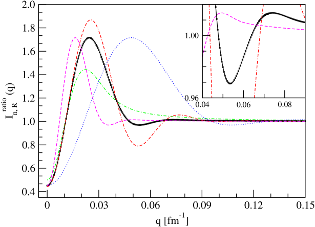
For $n>1$ a two-dimensional numerical integration is required to obtain $v_{c}^{R}(p^{\prime},p,x^{\prime},x)$. Due to strong oscillations of the integrand in (8) the big number of integration r-points is needed to achieve sufficient precision. This significantly increases the computer time needed for the t-matrix calculation, which has to be done on a big grid of $p,p^{\prime},x$ and $x^{\prime}$ points. Typically, we solve the Lippmann-Schwinger equation (1) using 120 p-points and 190 x-points for the sharply cut off potential and 95 p-points with 130 x-points for other screenings, what requires over $1.5\times 10^{8}$ calculations of the $v_{c}^{R}(p^{\prime},p,x^{\prime},x)$ function. The integration over $\phi$ in (8) can be performed with relatively small number of $\phi$-points and thus the whole numerical difficulty is shifted to calculation of $I_{n,R}(q)$. In order to speed it up we use the following method: in the first step we prepare the $I_{n,R}(q)$ on a grid of 300 q-points in the range of 0-100 fm^-1. In order to calculate the integral over $r$ we use the Filon’s integration formula abram which is dedicated to integrals of the product of the sine (or cosine) with some nonoscillatory function $f(x)$. The upper limit of integration $r_{max}$ is chosen sufficiently large so that the integrand approaches zero ($e^{-(\frac{r_{max}}{R})^{n}}=10^{-20}$). Since the resulting function $I_{n,R}(q)$ undergoes changes of 10 orders of magnitude in a rather small region of $q$, it is very difficult to handle it properly in further interpolations and integrations. A way out is to perform interpolations for the ratio $I_{n,R}^{ratio}(q)=I_{n,R}(q)/I_{1,R}(q)$ with analytically known $I_{1,R}=\frac{q}{q^{2}+R^{-2}}$. Variation of that ratio $I_{n,R}^{ratio}(q)$ is much more restricted, as shown in Fig.1, and we use its polynomial representation to get $I_{n,R}^{ratio}(q)$ at any value of $q$. For each value of $n$ and $R$ we divide the interpolation region into some optimal number of intervals, optimizing their length as well as degree of the polynomial. Typically we have 6 intervals while the degree of the polynomial varies between 6 to 12. This allows us to describe the oscillating function $I_{n,R}^{ratio}(q)$ with a sufficiently high precision, what is exemplified in Fig. 1 for n=3 and R=120 fm. In addition to the solid line for $I_{3,120}^{ratio}(q)$, the x-es in Fig.1 show the $I_{3,120}^{ratio}(q)$ values obtained from the polynomial formula. The agreement is perfect. The examples of the polynomial representation of $I_{n,R}^{ratio}(q)$ for two sets of screening parameters are given in the Appendix. The important and useful feature of $I_{n,R}^{ratio}(q)$, and thus also of the fit parameters, is its independence from the scattering energy. Due to that the interpolation can be done once for a given set of $n$ and $R$ values.

Once the $I_{n,R}^{ratio}(q)$ is calculated also $I_{n,R}(q)$ is known and the final integration over $\phi$ leads to $v_{c}^{R}(p^{\prime},p,x^{\prime},x)$. In our calculations we use typically a set of 500 gaussian points for the $\phi$-integration for all types of screening.

The properties of the resulting screened t-matrices are presented in the next Section.

III The screened Coulomb t-matrix properties

In this section the three-dimensional screened Coulomb t-matrix $t(p^{\prime},p,x=\cos(\theta))$ will be shown as a function of momenta $p,p^{\prime}$ at given scattering angle $\theta$. We choose as examples of backward, intermediate and forward angles the following values of $\theta$: $134^{\circ},45^{\circ},10^{\circ}$ and $5^{\circ}$.

In Fig. 2 the real and imaginary parts of the exponentially screened Coulomb t-matrix with n=4 and R=20 fm at E=13 MeV are shown. The real part of $t$ has a high and steep maximum at small momenta at $\theta=134^{\circ}$, which evolves to a ridge lying along diagonal $p^{\prime}=p$ for smaller angles. The spiky structure seen for the smallest angle comes only from the graphical representation on the finite grid of $p$ and $p^{\prime}$-points. The increasing range of the ridge shows that action of the screened Coulomb force becomes more and more important at bigger momenta when moving to smaller scattering angles. The imaginary part has a minimum at the on-shell point $p=p^{\prime}=p_{0}$ $(\approx 0.396$ fm^-1 for E=13 MeV$)$. Its absolute value is about one order of magnitude smaller than the maximum of the real part. The minimum of the imaginary part becomes deeper and narrower with decreasing angle.

The similar behaviour exists also for other values of the screening radius $R$. This is exemplified in Fig. 3 for $R=120$ fm. Taking higher values of $R$ leads to a more restricted range of momenta, at which the real part of $t$ takes large values. However, the maximum of $Re(t)$ is much higher than for $R=20$ fm. Also the range of momenta, where $Im(t)$ has the deep minimum is much smaller than for $R=20$ fm.

In Figs. 4 and 5 the t-matrix for the sharp cut-off screening at E=13 MeV is shown for two values of cut-off parameter: R=20 fm and R=80 fm, respectively. The general picture is similar to that for the exponential screening, however, some oscillations are visible for both real and imaginary parts of the t-matrix. For the real part they are clearly visible at small momenta. For the imaginary part at bigger scattering angles they are relatively large, when compared to the absolute minimum of $Im(t)$ and decrease with decreasing angles.

The t-matrices obtained using the localized screening of Eq. (5) are shown in Fig. 6 ($R=9$ fm) and Fig. 7 ($R=55$ fm). These values of the localized screening range parameter $R=9$ $(55)$ fm correspond roughly to the values of the screening radius $R=20$ $(120)$ fm for the exponential screening. The resulting t-matrices are very similar to those obtained with the exponential screening at the same angles.

For the exponential screening we investigated the dependence of the screened Coulomb t-matrix on the value of the screening parameter $n$. We found only weak dependence, as exemplified in Fig. 8 where t-matrices at $\theta=10^{\circ}$ are shown for $n=2$ and $n=3$. This picture can be further supplemented by parts of Fig. 2 ($n=4$) and Fig. 4 (sharp cut-off, what corresponds to infinite value of $n$) at the same angle. It is seen that there is only small decreasing of the height of the diagonal ridge for the real part of the t-matrix at the smallest momenta. The minimum of the imaginary part becomes narrower and deeper with increasing $n$.

Finally, we checked, how good is the approximation of the three-dimensional screened Coulomb t-matrix by the screened Coulomb potential alone. To that aim we looked at the ratio

$$\Delta\equiv\frac{t_{c}^{R}(p^{\prime},p,x)-V_{c}^{R}(p^{\prime},p,x)}{V_{c}^{R}(p^{\prime},p,x)}$$

In Fig. 9 we show $\Delta$ at different scattering angles, obtained for the exponential screening with $R$=120 fm and $n$=4 at $E=13$ MeV. At all angles the real part of $\Delta$ does not exceed 12%. The imaginary part of $\Delta$ is below 3% for all $p$ and $p^{\prime}$ values what emphasizes the smallness of the imaginary part and would indicate on validity of approximation $t_{c}^{R}$ by pure screened Coulomb potential $V_{c}^{R}$. The differences between the values of $t_{c}^{R}$ and $V_{c}^{R}$ are biggest for $p,p^{\prime}<p_{0}$ and around $p=p_{0}$ or $p^{\prime}=p_{0}$. It means that in those regions of momenta the approximation of the screened Coulomb t-matrix by the corresponding screened Coulomb potential is rather poor.

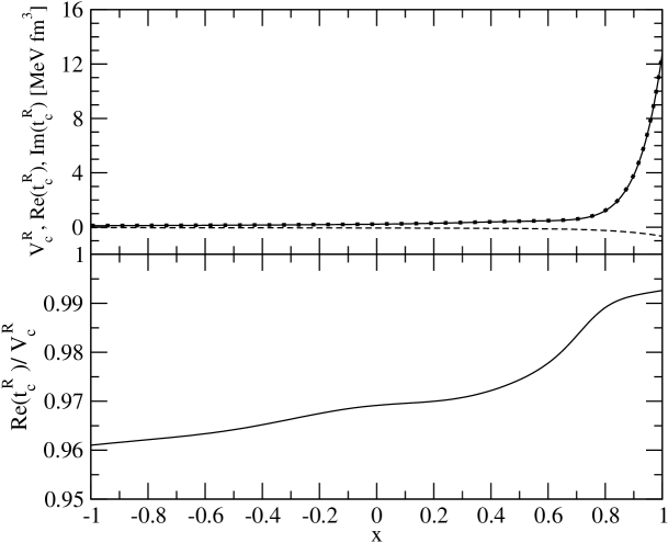
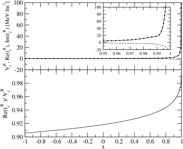
For the on-shell screened Coulomb t-matrix elements $<p_{0}\hat{p^{\prime}}|t_{c}^{R}(\frac{p_{0}^{2}}{m})|p_{0}\hat{p}>$ obtained with exponential screening we show quality of the Born approximation in Figs. 10 and 11. There the screened Coulomb potential $V_{c}^{R}(p_{0},p_{0},x)$ together with t-matrix elements are shown as a function of cosine of scattering angle $\theta$. The screening parameters are $n=4$ and $R=20$ fm for Fig. 10 and $n=4$ and $R=120$ fm for Fig. 11

The real part of the screened Coulomb t-matrix (solid line) and the screened Coulomb potential (dotted line) are close to each other, and their ratio does not exceed 4% of $V_{c}^{R}$ for the screening range $R=20$ fm and increases up to about 10% when the screening radius reaches $R=120$ fm. In both cases the imaginary part of the t-matrix is much smaller than its real part and becomes important only at very small scattering angles. The real part of the t-matrix is in all cases somewhat smaller than the corresponding potential matrix element.

IV The three-dimensional t-matrix from the partial wave decomposition

In this section we would like to compare the on-shell elements of the three-dimensional screened Coulomb t-matrix obtained directly from Eq.(1) with its value derived from solutions of the partial wave decomposed Lippmann-Schwinger equation $<p,l|t|p^{\prime},l>$. The latter is given as a sum of contributions from different angular momenta $l$

$$t^{pw}(\vec{p},\vec{p^{\prime}},x)\equiv\sum_{l=0}^{l_{max}}\frac{2l+1}{4\pi}P_{l}(x)<p,l|t|p^{\prime},l>,$$ (10)

where $P_{l}(x)$ is the Legendre polynomial of the cosine of the scattering angle, $x=\hat{p}\cdot\hat{p^{\prime}}$, and $l_{max}$ should be high enough to give convergent result at given energy and screening. The $<p,l|t|p^{\prime},l>$ partial wave t-matrix element is a solution of the one-dimensional Lippmann-Schwinger equation with the screened Coulomb potential driven by its partial wave element:

$$<p,l|V_{c}^{R}|p^{\prime},l>\equiv\frac{2\alpha}{\pi}\int_{0}^{\infty}dr\;r\;j_{l}(pr)e^{-(\frac{r}{R})^{n}}j_{l}(p^{\prime}r)\;.$$ (11)

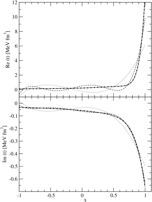
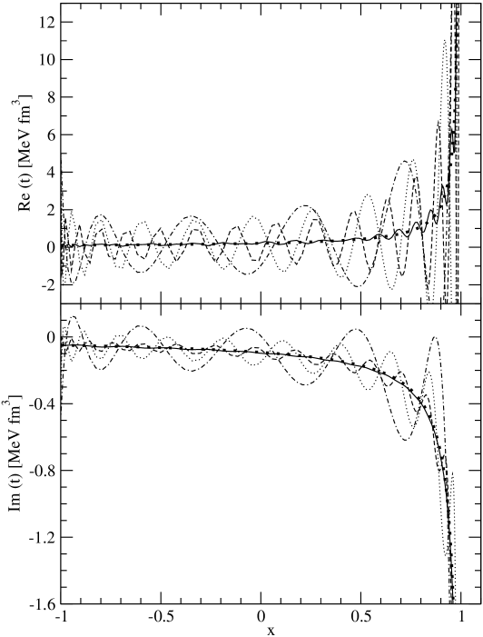
In Fig.12 we show convergence of the result with respect to $l_{max}$ for $l_{max}=3,5$ and $10$. The partial wave generated screened Coulomb t-matrix is compared to the exponentially screened Coulomb t-matrix obtained directly from Eq. (1) with $n=4$ and $R=20$ fm at E=13 MeV. For such relatively small screening radius $R$ it is sufficient to restrict to partial waves up to $l_{max}=10$ only to reproduce the full 3-dimensional t-matrix (thick dotted line). However, the number of partial waves needed to reproduce the full three-dimensional t-matrix increases rapidly with increasing screening radius. This is exemplified in Fig.13 for $R=120$ fm, where partial wave generated results with $l_{max}=10,20,30$ and $50$ are shown together with the full solution. It is clearly seen that even taking $l_{max}=50$ is still not enough to describe with sufficient precision the full three-dimensional screened Coulomb t-matrix. This shows the importance of the direct three-dimensional solution of Eq.(1), which avoids problems caused by very slow convergence of the partial wave expansion for big screening radii.

V Summary

In this paper we investigated numerically behaviour of the three-dimensional screened Coulomb t-matrix using different types of screening. Such t-matrix is solution of the three-dimensional Lippmann-Schwinger equation and is an important component of a recently developed novel approach to include the pp Coulomb force into the three-nucleon Faddeev calculations witala ; witala2 . The direct application of the three-dimensional screened Coulomb t-matrix decreases substantially number of partial waves needed in 3N calculations reducing them to the number of partial waves needed to get converged results in case when only nuclear part of the potential is acting. The presented numerical procedure enables to get precise values of the three-dimensional screened Coulomb t-matrix for any form of the screening.

We have also presented behaviour of the screened Coulomb t-matrix for different types of screening and for different values of screening parameters. The resulting t-matrices are similar. Only the t-matrix based on the sharply cut off Coulomb potential reveals oscillations, which are absent for other types of screening. Those oscillations cause, that numerical requirements on computer resources are bigger in that case. The behaviour of the real and imaginary parts of the three-dimensional screened Coulomb t-matrix with varying scattering angle is clearly seen in given examples. The range of relative momenta, where the real part of $t$ is important rapidly grows with decreasing scattering angle for all types of screening. Contrary, the imaginary part of $t$ becomes more localized with decreasing scattering angle but the depth of its minimum grows.

The presented results exemplify, that the three-dimensional screened Coulomb t-matrix can be obtained numerically in a reliable way for any type of screening making it a valuable input in three-body calculations.

VI Appendix

In the following tables we give values of parameters $a_{k}$ for the polynomial representations of the $I_{n,R}^{ratio}(q)=\sum_{k}a_{k}q^{k}$ in case of exponential screening and two sets of $(n,R)$ parameters: $(n=2,R=20)$ in Tab. 1 and $(n=4,R=120)$ in Tab. 2. The $k$ (first column) gives a power of q which goes with the corresponding $a_{k}$ factor given in next columns for different ranges of q [fm^-1].

k	q$<$0.4	0.4$<$q$<$0.4825	0.4825$<$q$<$0.98	0.98$<$q$<$1.725	1.725$<$q$<$10.5	10.5$<$q$<$100
0	0.5000125677171	2.400709537574	3.921200500830	1.100526033577	1.015402877247	1.000334483409
1	-0.006479230796918	-11.71854218076	-37.98859669416	-0.2600475901233	-0.1503793799690E-01	-0.4682291329186E-04
2	167.3502341712	42.56921618797	242.8850249646	0.2987640252234	0.6468810517976E-02	0.2854148534117E-05
3	-20.31247086770	-80.71301847419	-974.8378775605	-0.1809241210266	-0.1511703363356E-02	-0.9406333859035E-07
4	-12352.87853580	78.54728957584	2694.796660079	0.5644212648115E-01	0.2040113688732E-03	0.1787524617018E-08
5	36456.32220409	-31.11252021404	-5362.934658952	-0.7169472025225E-02	-0.1584593947154E-04	-0.1954522705295E-10
6	-524160.9711593	-	7842.047876700	-	0.6567867383073E-06	0.1140554415044E-12
7	15708513.64668	-	-8464.239235675	-	-0.1124054147047E-07	-0.2748652734470E-15
8	-165490836.2729	-	6679.063924791	-	-	-
9	931536159.6442	-	-3752.307134393	-	-	-
10	-3219232757.359	-	1423.137799525	-	-	-
11	7104191720.650	-	-326.9144001002	-	-	-
12	-9827857786.235	-	34.37700645114	-	-	-
13	7804143302.566	-	-	-	-	-
14	-2723712664.926	-	-	-	-	-

Table 1: Parameters for the polynomial representation of $I_{n,R}^{ratio}(q)$ for exponential screening with $n=2$ and $R=20$.

k	Q$<$0.0735	0.0735$<$q$<$0.11	0.11$<$q$<$0.148	0.148$<$q$<$0.4755	0.4755$<$q$<$1.49	1.49$<$q$<$100
0	0.4430751038110	-61.12120265116	17222.40652970	1.014501500770	1.002164118242	1.000039812743
1	0.1624327164522	3122.555537517	-1665157.950661	-0.1499375990712	-0.8401588857950E-02	-0.1260392857265E-04
2	5657.908456700	-61815.86410617	72913086.23221	0.6806385287457	0.1422552507692E-01	0.1308082855220E-05
3	37890.24852747	603243.9054240	-1912425443.395	-1.605992271344	-0.1246326266740E-01	-0.6209139096908E-07
4	-14459376.10638	-2904646.753554	33474324944.51	1.925075383945	0.5526732459266E-02	0.1534201149986E-08
5	613454088.3275	5524183.167489	-412042007272.1	-0.9274592364796	-0.9817848874961E-03	-0.2041445354694E-10
6	-34028042154.54	-	3658148517742.	-	-	0.1386086594813E-12
7	1709808009779.	-	-0.2360571796460E+14	-	-	-0.3765737840762E-15
8	-0.5319386618092E+14	-	0.1098886587674E+15	-	-	-
9	0.1051045675524E+16	-	-0.3598714293204E+15	-	-	-
10	-0.1399718714098E+17	-	0.7868023497509E+15	-	-	-
11	0.1294364258655E+18	-	-0.1030692803221E+16	-	-	-
12	-0.8173922266757E+18	-	0.6113583130648E+15	-	-	-
13	0.3207993078724E+19	-	-	-	-	-
14	-0.5891645069211E+19	-	-	-	-	-

Table 2: The same as in Tab 1 but for $n=4$ and $R=120$.

Figure 1: (color online) The $I_{n,R}^{ratio}(q)$ for different combinations of screening parameters and the quality of polynomial fit for $I_{3,120}^{ratio}(q)$. The solid (black) line represents $I_{3,120}^{ratio}(q)$ calculated by direct integration over $r$ in (8) as a function of momenta q. The black x-es show the values of $I_{3,120}^{ratio}(q)$ obtained from its polynomial representation. Other curves: dash-dotted (green), double-dashed-dotted (red), dotted (blue) and dashed (magenta) represents $I_{2,120}^{ratio},I_{4,120}^{ratio},I_{3,60}^{ratio}$ and $I_{3,180}^{ratio}$, respectively. For $0.15<q<100$ fm the $I_{n,R}^{ratio}(q)$ is practically equal 1.

Figure 2: The real (left) and imaginary (right) parts of the screened Coulomb t-matrix $t(p,p^{\prime},x=\cos(\theta))$ at E=13 MeV for different scattering angles $\theta=$ $134^{\circ}$(1-st row), $\theta=45^{\circ}$(2-nd row), $\theta=10^{\circ}$(3-rd row) and $\theta=5^{\circ}$(4-th row). The exponential screening with R=20 fm and n=4 has been applied.

Figure 3: The same as in Fig.2 but for R=120 fm.

Figure 4: The same as in Fig.2 but for the sharp cut-off screening of Eq.(3) with R=20 fm at E=13 MeV.

Figure 5: The same as in Fig.2 but for the sharp cut-off screening of Eq.(3) with R=80 fm at E=13 MeV.

Figure 6: The same as in Fig.2 but for the localized screening of Eq.(5) with R=9 fm.

Figure 7: The same as in Fig.2 but for the localized screening of Eq.(5) with R=55 fm.

Figure 8: The real and imaginary parts of the exponentially screened Coulomb t-matrix at E=13 MeV for the scattering angle $\theta$=$10^{\circ}$, R=20 fm and for two values of the screening parameter $n=2$ (up) and $n=3$ (down).

Figure 9: The real (left) and imaginary (right) parts of the ratio $\Delta=(t-v)/v$ (see text) for different scattering angles $\theta$: $134^{\circ}$(1-st row), $45^{\circ}$(2-nd row), $10^{\circ}$(3-rd row) and $5^{\circ}$(4-th row) for the exponential screening with R=20 fm and n=4 at E=13 MeV.

Figure 10: The real (solid line) and imaginary (dashed line) parts of the on-shell exponentially screened Coulomb t-matrix $t_{c}^{R}(p_{0},p_{0},x)$ at E=13 MeV as a function of the cosine of scattering angle $\theta$ ($x=\cos(\theta)$) (upper part). The dotted line is the corresponding screened Coulomb potential $V_{c}^{R}(p_{0},p_{0},x)$. In the lower part of figure the ratio $Re(t_{c}^{R})/V_{c}^{R}$ is shown. The parameters of the screening are R=20 fm and n=4.

Figure 11: The same as in Fig.10 but for R=120 fm.

Figure 12: The convergence in the partial waves of the exponentially screened Coulomb t-matrix at E=13 MeV. The real and imaginary parts of the on-shell elements of the three-dimensional screened Coulomb t-matrix are given by thick dotted line. The other lines represent partial wave generated results obtained by summation of partial waves up to $l_{max}=3$ (dotted), $l_{max}=5$ (dashed) and $l_{max}=10$ (solid). The screening parameters are $n=4$ and $R=20$ fm.

Figure 13: The same as in Fig. 12 but for R=120 fm. The partial waves generated results are obtained by summing up to $l_{max}=10$ (dash-dotted), $l_{max}=20$ (dotted), $l_{max}=30$ (dashed) and $l_{max}=50$ (solid). The thick dotted line represents as before the three-dimensional screened Coulomb t-matrix.

References

- (1) C. M. Vincent and S. C. Phatak, Phys. Rev. C10, 391 (1974).
- (2) A. Kievsky, M. Viviani, and S. Rosati, Phys. Rev. C 52, R15 (1995).
- (3) A. Deltuva, A. C. Fonseca, and P. U. Sauer, Phys. Rev. C71, 054005 (2005).
- (4) H.Witała, R.Skibiński, J.Golak, W.Glöckle, Eur. Phys. J. A41, 369 (2009)
- (5) A. Deltuva, A. C. Fonseca, and P. U. Sauer, Phys. Rev. C72, 054004 (2005).
- (6) H.Witała, R.Skibiński, J.Golak, W.Glöckle, Eur. Phys. J. A41, 385 (2009).
- (7) Ch. Elster, J.H. Thomas, and W. Glöckle, Few-Body Systems 24, 55 (1998).
- (8) R. Skibiński, J. Golak, H.Witała and W. Glöckle, Eur. Phys. J. A (2009).
- (9) L.P. Kok and H. van Haeringen, Phys. Rev. Lett. 46, 1257, (1981).
- (10) H. van Haeringen, Charged Particle Interactions, Theory and Formulas, Coulomb Press Leyden, 1985.
- (11) M. Rodriguez-Gallardo, A. Deltuva, E. Cravo, R. Crespo, A.C. Fonseca, Phys. Rev. C78 034602 (2008).
- (12) Handbook of mathematical functions, ed. M. Abramowitz and I. A. Stegun, Dover Publ., N. Y. 1972.